| Issue |
A&A
Volume 556, August 2013
|
|
|---|---|---|
| Article Number | A90 | |
| Number of page(s) | 7 | |
| Section | Cosmology (including clusters of galaxies) | |
| DOI | https://doi.org/10.1051/0004-6361/201321623 | |
| Published online | 01 August 2013 | |
The high-redshift star formation rate derived from gamma-ray bursts: possible origin and cosmic reionization
1
School of Astronomy and Space Science, Nanjing University, 210093 Nanjing, PR China
e-mail: This email address is being protected from spambots. You need JavaScript enabled to view it.
2
Department of Physics, The University of Hong Kong, Pokfulam Road, Hong Kong, PR China
3
Key Laboratory of Modern Astronomy and Astrophysics (Nanjing University), Ministry of Education, 210093 Nanjing, PR China
Received:
2
April
2013
Accepted:
4
June
2013
Abstract
The collapsar model of long gamma-ray bursts (GRBs) indicates that they may trace the star formation history, so long GRBs may be a useful tool for measuring the high-redshift star formation rate (SFR). The collapsar model explains GRB formation via the collapse of a rapidly rotating massive star with M > 30 M⊙ into a black hole, which may imply a decrease in SFR at high redshift. However, we find that the Swift GRBs during 2005 to 2012 are biased when tracing the SFR, including a factor about (1 + z)0.5, which agrees with recent results. After taking this factor, the SFR derived from GRBs does not show a steep drop up to z ~ 9.4. We consider the GRBs produced by rapidly rotating metal-poor stars with low masses to explain the high-redshift GRB rate excess. The chemically homogeneous evolution scenario (CHES) of rapidly rotating stars with mass higher than 12 M⊙ is recognized as a promising path towards collapsars in connection with long GRBs. Our results indicate that the stars in the mass range 12 M⊙ < M < 30 M⊙ for low enough metallicity Z ≤ 0.004 with the GRB efficiency factor 10-5 can fit the derived SFR with good accuracy. Combining these two factors, we find that the conversion efficiency from massive stars to GRBs is enhanced by a factor of 10, which may explain the excess of the high-redshift GRB rate. We also investigate the cosmic reionization history using the derived SFR. The GRB-inferred SFR would be sufficient to maintain cosmic reionization over 6 < z < 10 and reproduce the observed optical depth of Thomson scattering to the cosmic microwave background.
Key words: gamma rays: general / stars: formation / dark ages, reionization, first stars
© ESO, 2013
1. Introduction
Gamma-ray bursts (GRBs) are the brightest electromagnetic explosions in the universe (for a recent review, see Gehrels et al. 2009). Because of their very high luminosity, GRBs can be detected out to the edge of the visible Universe (Ciardi & Loeb 2000; Lamb & Reichart 2000; Bromm & Loeb 2002, 2006). The farthest GRB to date is GRB 090429B with a photometric redshift z = 9.4 (Cucchiara et al. 2011), significantly higher than those of the most distant quasars. This property makes GRBs indispensable beacons for studying the early universe, including the star formation rate (SFR; Totani 1997; Wijers et al. 1998; Porciani & Madau 2001; Bromm & Loeb 2002, 2006), the intergalactic medium (IGM; Barkana & Loeb 2004; Inoue et al. 2007; McQuinn et al. 2008), and metal enrichment history (Savaglio 2006; Wang et al. 2012). In addition, GRBs have been used as standard candles to constrain cosmological parameters and dark energy (Dai et al. 2004; Schaefer 2007; Wang et al. 2011).
The most popular theoretical model of long-duration GRBs is the collapse of a massive star to a black hole (Woosley 1993). Observations also show that GRBs are associated with Type Ib/c supernovae (Stanek et al. 2003; Hjorth et al. 2003), so GRBs provide a complementary technique for measuring the SFR history (Totani 1997; Wijers et al. 1998; Porciani & Madau 2001). Recent studies have shown that Swift GRBs do not trace the star formation history measured by traditional means exactly, but include an additional evolution (Le & Dermer 2007; Salvaterra & Chincarini 2007; Kistler et al. 2008; Yüksel et al. 2008; Wang & Dai 2009; Wanderman & Piran 2010; Qin et al. 2010; Cao et al. 2011; Robertson & Ellis 2012; but see Elliott et al. 2012). The SFR inferred from the high-redshift (z > 6) GRBs seems to be too high in comparison with the one obtained from some high-redshift galaxy surveys (Kistler et al. 2009; Bouwens et al. 2009). Kistler et al. (2008) found that there are about four times as many GRBs at redshift z ~ 4 than expected from star formation measurements. They claimed that some unknown mechanism is leading to an enhancement about (1 + z)δ (δ = 1.5) in the observed rate of high-redshift GRBs. Using more Swift data, Kistler et al. (2009) find a slightly lower value of enhancement about (1 + z)1.2. Robertson & Ellis (2012) find the value of δ is about 0.5 by comparing the cumulative redshift distribution of GRBs and SFR. On the other hand, Elliott et al. (2012) find that the value of δ is about zero using a small sample of GRBs. In order to explain this discrepancy, many models have been proposed. Li (2008) explained the observed discrepancy between the GRB rate history and the SFR history as due to cosmic metallicity evolution (Langer & Norman 2006), by assuming that long GRBs tend to occur in galaxies with low metallicities. Cheng et al. (2010) suggest that this discrepancy could be solved if some high-redshift GRBs are produced by superconducting cosmic strings. Wang & Dai (2011) use an evolving initial mass function (IMF) of stars to explain the GRB redshift distribution. Virgili et al. (2011) discuss the possibility that the evolution of the GRB luminosity function break with redshift may explain this discrepancy. Observations also show differences in the population of GRB host galaxies compared to expectations for an unbiased star-formation tracer (Tanvir et al. 2004; Fruchter et al. 2006; Svensson et al. 2010).
In this paper, we study the SFR history derived from GRBs. First we use the Swift GRB sample to test the evolution of GRB rate relative to SFR. If GRBs trace star formation in the universe without bias, the ratio of the GRB rate to the SFR would not be expected to vary with redshift. We find that this ratio is proportional to (1 + z)0.5. The index is less than the value of Kistler et al. (2009). We also derive the high-redshift SFR using Swift GRB sample by correcting this evolution. Then, we consider the rapidly rotating metal-poor stars with lower masses than the critical mass Mcri ~ 30 M⊙ to see if they can produce GRBs to explain the discrepancy between high-redshift SFR and the GRB rate. The collapsar model indicates that stars with mass higher than 30 M⊙ can produce GRBs (Woosley 1993; Bissaldi et al. 2007; Raskin et al. 2008). Observation also shows that the progenitor of GRB 060505 has a mass above 30 M⊙ (Thöne et al. 2008). Yoon & Langer (2005) investigated the evolution of rotating single stars in the mass range 12 M⊙ < M < 60 M⊙ at low metallicity. They find that if the initial spin rate is high enough, the time scale for rotationally induced mixing becomes shorter than the nuclear time scale. The star may evolve in a quasi-chemically homogeneous way. In particular, for low enough metallicity, this type of evolution can lead to retention of sufficient angular momentum in cores to produce GRBs according to the collapsar scenario. Last, we calculate the impact of this GRB-inferred SFR on the reionization history, including the optical depth of electron scattering to the cosmic microwave background.
The structure of this paper is arranged as follows. In the next section, we compile the Swift GRB sample until GRB 110403 and test the evolution of GRB rate. The SFR derived from GRBs is given in Sect. 3. We show the model of GRBs from chemically homogeneous evolution scenario and the influence on high-redshift SFR derived from GRBs in Sect. 4. We compute the reionization history with this GRB-inferred SFR in Sect. 5. We conclude with a summary in Sect. 6.
2. The latest GRB sample
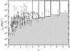 |
Fig. 1 Distribution of the isotropic-equivalent luminosity for 157 long-duration Swift GRBs. The GRB subsamples used to estimate the SFR are outlined. The shaded area approximates the detection threshold of Swift BAT. |
The expected redshift distribution of GRBs is  (1)where
F(z) represents the ability both to detect the trigger
of burst and to obtain the redshift, ε(z) accounts for the
fraction of stars producing GRBs, and
(1)where
F(z) represents the ability both to detect the trigger
of burst and to obtain the redshift, ε(z) accounts for the
fraction of stars producing GRBs, and  is the SFR density. The F(z) can be treated as constant
when we consider the bright bursts with luminosities sufficient to be detected within an
entire redshift range, so
F(z) = F0. GRBs that are
unobservable due to beaming are accounted for through
⟨ fbeam ⟩ . The ε(z) can be
parameterized as
ε(z) = ε0(1 + z)δ,
where ε0 is an unknown constant that includes the absolute
conversion from the SFR to the GRB rate in a given GRB luminosity range. Kistler et al.
(2008) find the index δ = 1.5 from
63 Swift GRBs. A little lower value, δ = 1.2, was inferred
using 119 Swift GRBs (Kistler et al. 2009). In a flat universe, the comoving volume is calculated by
is the SFR density. The F(z) can be treated as constant
when we consider the bright bursts with luminosities sufficient to be detected within an
entire redshift range, so
F(z) = F0. GRBs that are
unobservable due to beaming are accounted for through
⟨ fbeam ⟩ . The ε(z) can be
parameterized as
ε(z) = ε0(1 + z)δ,
where ε0 is an unknown constant that includes the absolute
conversion from the SFR to the GRB rate in a given GRB luminosity range. Kistler et al.
(2008) find the index δ = 1.5 from
63 Swift GRBs. A little lower value, δ = 1.2, was inferred
using 119 Swift GRBs (Kistler et al. 2009). In a flat universe, the comoving volume is calculated by  (2)where
the comoving distance is
(2)where
the comoving distance is  (3)In
the calculations, we use Ωm = 0.27, ΩΛ = 0.73, and
H0 = 71 km s-1 Mpc-1 from the
Wilkinson Microwave Anisotropy Probe (WMAP) seven-year data (Komatsu
et al. 2011).
(3)In
the calculations, we use Ωm = 0.27, ΩΛ = 0.73, and
H0 = 71 km s-1 Mpc-1 from the
Wilkinson Microwave Anisotropy Probe (WMAP) seven-year data (Komatsu
et al. 2011).
We use the latest Swift long-duration GRB sample till GRB 110403. The data
is taken from Butler et al. (2007, 2010) and a website1. The isotropic-equivalent luminosity of a GRB can be obtained by  (4)The distribution of
Liso for 157 GRBs in the sample is shown in Fig. 1. We use the same luminosity cuts in these redshift bins
as Kistler et al. (2009). The shaded area
approximates the detection threshold of Swift BAT, which can be calculated
as follows. The luminosity threshold can be approximated by a bolometric energy flux limit
Flim = 1.2 × 10⁻⁸ erg cm-2
s-1. The luminosity threshold is then
(4)The distribution of
Liso for 157 GRBs in the sample is shown in Fig. 1. We use the same luminosity cuts in these redshift bins
as Kistler et al. (2009). The shaded area
approximates the detection threshold of Swift BAT, which can be calculated
as follows. The luminosity threshold can be approximated by a bolometric energy flux limit
Flim = 1.2 × 10⁻⁸ erg cm-2
s-1. The luminosity threshold is then  (5)where
DL is the luminosity distance to the burst.
(5)where
DL is the luminosity distance to the burst.
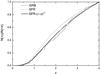 |
Fig. 2 Cumulative distribution of 92 Swift GRBs with Liso > 1051 erg s-1 in z = 0−4 (stepwise solid line). The dashed line shows the GRB rate inferred from the star formation history of Hopkins & Beacom (2006). The solid line shows the GRB rate inferred from the star formation history including (1 + z)0.5 evolution. |
To test the GRB rate relative to the SFR, we had to choose bursts with high luminosities, because only bright bursts can be seen at low- and high-redshifts, so we chose the luminosity cut Liso > 1051 erg s-1 (Yüksel et al. 2008) in the redshift bin 0–4. This removes many low-redshift, low-Liso bursts that could not have been seen at higher redshift. Because the SFR at high redshift is poorly known (Bouwens et al. 2012; Oesch et al. 2013; Coe et al. 2013), we chose the redshift range 0 < z < 4, where SFR is measured well. We have 92 GRBs in this subsample. We used the SFR history from Hopkins & Beacom (2006) to compare the predicted and observed cumulative GRB distributions in Fig. 2. We find that the Kolmogorov-Smirnov statistic is minimized for δ = 0.5, which is consistent with Robertson & Ellis (2012). At the 2σ confidence level, the value of δ is in the range −0.15 < δ < 1.6. Our result is lower than the values in Kistler et al. (2009). This may account for the different GRB sample. The GRB sample observed by Swift during 2005-2012 is used in this paper. This bias must be taken into account when one relates the GRB rate to the SFR.
3. The SFR derived from GRBs
In this section, we use the same method as Yüksel et al. (2008) to calculate the SFR rate from GRBs. Because only very bright bursts can be
seen from all redshifts, we use the same luminosity cuts as Kistler et al. (2009), as shown in Fig. 1. The number counts in redshift bins z = 4−5, 5–6, 6–7, 7–8.5,
and 8.5–10 are 10, 4, 2, 1, and 1, respectively. In the redshift bin of 8.5–10, there is
only one GRB named GRB 090429B with photometric redshift z ~ 9.4, although
there is a low-probability tail to somewhat lower redshifts (Cucchiara et al. 2011). The bin choice of our work is different with those
of Robertson & Ellis (2012). We choose
redshift bins uniform in z, and also ensure that the number of GRBs in each
bin is equal to or larger than one. We also calculate the SFR using bin choice of Robertson
& Ellis (2012), and find that the result is a
little different than with the current bin choice. The GRBs in z = 1−4
act as a “control group” to constrain the GRB to SFR conversion, since this redshift bin has
both good SFR measurements and good GRB counts. We calculate the theoretically predicated
number of GRBs in this bin as 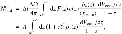 (6)where
A = Δt ΔΩ F0/4π⟨fbeam⟩
depends on the total observed time of Swift, Δt, and the
angular sky coverage, ΔΩ. The theoretical number of GRBs in redshift bin
z1 − z2 can be written as
(6)where
A = Δt ΔΩ F0/4π⟨fbeam⟩
depends on the total observed time of Swift, Δt, and the
angular sky coverage, ΔΩ. The theoretical number of GRBs in redshift bin
z1 − z2 can be written as
 (7)where
  is the average SFR density in the redshift range
z1 − z2. Representing the
predicated numbers,
is the average SFR density in the redshift range
z1 − z2. Representing the
predicated numbers,  with the observed
GRB counts,
with the observed
GRB counts,  , we obtain
the SFR in the redshift range
z1 − z2,
, we obtain
the SFR in the redshift range
z1 − z2,  (8)In the calculation, we
assume that the value of δ is constant during the full redshift range. The
derived SFRs from GRBs are shown in Fig. 3. Error bars
correspond to 68% Poisson confidence intervals for the binned events (Gehrels 1986). The high-redshift SFRs obviously decrease with
increasing redshifts, although an oscillation may exist. We find that the SFR at
z > 4.48 is proportional to
(1 + z)-3 using minimum χ2 method,
which is shown in Fig. 3. Because we use different
cosmological parameters from Hopkins & Beacom (2006) (Ωm = 0.3, ΩΛ = 0.7
and H0 = 70 km s-1 Mpc-1), SFR
conversion between different cosmology models must be considered. The conversion factor for
a given redshift range can be expressed as (Hopkins 2004)
(8)In the calculation, we
assume that the value of δ is constant during the full redshift range. The
derived SFRs from GRBs are shown in Fig. 3. Error bars
correspond to 68% Poisson confidence intervals for the binned events (Gehrels 1986). The high-redshift SFRs obviously decrease with
increasing redshifts, although an oscillation may exist. We find that the SFR at
z > 4.48 is proportional to
(1 + z)-3 using minimum χ2 method,
which is shown in Fig. 3. Because we use different
cosmological parameters from Hopkins & Beacom (2006) (Ωm = 0.3, ΩΛ = 0.7
and H0 = 70 km s-1 Mpc-1), SFR
conversion between different cosmology models must be considered. The conversion factor for
a given redshift range can be expressed as (Hopkins 2004)  (9)where
Dcom is given in Eq. (3). At the redshift range z = 4−5, the value of conversion
factors in these two cosmological models are very similar. The relative error is less than
4%, so our results are insensitive to the choice of WMAP7 cosmology. The new determination
of SFR is slight smaller than the result given by Kistler et al. (2009). There are two reasons for this situation. First, we derive a
smaller evolution-factor index δ. Second, we updated the Swift
GRB sample. In past three years, Swift has observed many more GRBs
with medium redshifts than GRBs with high redshifts, so the ratio
(9)where
Dcom is given in Eq. (3). At the redshift range z = 4−5, the value of conversion
factors in these two cosmological models are very similar. The relative error is less than
4%, so our results are insensitive to the choice of WMAP7 cosmology. The new determination
of SFR is slight smaller than the result given by Kistler et al. (2009). There are two reasons for this situation. First, we derive a
smaller evolution-factor index δ. Second, we updated the Swift
GRB sample. In past three years, Swift has observed many more GRBs
with medium redshifts than GRBs with high redshifts, so the ratio  is lower
than in Kistler et al. (2009).
is lower
than in Kistler et al. (2009).
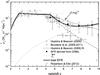 |
Fig. 3 Cosmic star formation history. The gray points are taken from Hopkins & Beacom (2006), the dashed line shows their fitting result. The triangular points are from Bouwens et al. (2009, 2011). The open circles are taken from Robertson & Ellis (2012). The filled circles are the SFR derived from GRBs in this work. The dotted line shows the effect SFR calculated from Eq. (19). The thick solid line shows the combination of dashed and dotted lines. |
Ishida et al. (2011) used the principal component analysis method to measure the high-redshift SFR from the distribution of GRBs and find that the SFR at z ~ 9.4 could be up to 0.01 M⊙ yr-1 Mpc-3. Robertson & Ellis (2012) constrained the SFR using GRBs by considering the contribution of “dark” GRBs. They find that the high-redshift SFR derived from GRBs can vary by a factor of 4 using different values of δ. Their results for δ = 0.5 are shown in Fig. 3. Our result can be marginally consistent with Robertson & Ellis (2012). Elliott et al. (2012) chose 43 GRBs by selecting GRBs that have been detected by GROND within four hours after the Swift BAT trigger and that exhibited an X-ray afterglow. They find the linear relationship between GRB rate and SFR using this small sample. Johnson et al. (2013) used high-resolution cosmological simulations to study the high-redshift SFR. Our result is consistent with Johnson et al. (2013) at z ≤ 10. But at z ≥ 10, they find that the SFR is reduced by up to an order of magnitude owing to the molecule-dissociating stellar radiation.
4. GRBs from rapidly rotating metal-poor stars and their influence on SFR
The collapsar model explains GRB formation via the collapse of a rapidly rotation massive iron core into a black hole (Woosley 1993). This collapse model requires the initial mass of the massive stars with masses higher than about 30 M⊙ (Woosley 1993; Bissaldi et al. 2007). Yoon & Langer (2005) and Woosley & Heger (2006) show that at low metallicity, quasi-chemically-homogeneous evolution of rapidly rotating stars with low masses can lead to the formation of rapidly rotating helium stars, which satisfies all the requirements of the collapsar scenario. Because the rotation affects the evolution of stars significantly, especially through rotationally induced chemical mixing (Maeder & Meynet 2000; Heger et al. 2000), the star remains chemically homogeneous evolution scenario (CHES). The CHES is recognized as a promising path towards collapsars in connection with long GRBs. Yoon et al. (2006) show that at low metallicity (Z ≤ 0.004), the quasi-chemically-homogeneous evolution of rapidly rotating stars with masses higher than 12 M⊙ can lead to long GRBs2. We call this type of GRB a chemically homogeneous GRB (CHG) below. If stars in the same mass range have high metallicities and slow rotation, they will die as type II supernovae (see Fig. 3 of Yoon et al. 2006). This picture has also been confirmed by observation (Fruchter et al 2006).
We study the rate of CHG from the chemically homogeneous evolution scenario as follows. The
most widely used functional form for the initial mass function (IMF) is the one proposed by
Salpeter (1955):  (10)where
ASalpeter = 0.06 is the normalization constant derived from
(10)where
ASalpeter = 0.06 is the normalization constant derived from  (11)We use
mlow = 0.1 M⊙ and
mup = 120 M⊙. We consider
stars with masses between 12 M⊙ and
30 M⊙. Because the stars with masses
M ≥ 30 M⊙ can produce GRBs through
conventional collapse model (Woosley 1993), so the
rate of CHG is
(11)We use
mlow = 0.1 M⊙ and
mup = 120 M⊙. We consider
stars with masses between 12 M⊙ and
30 M⊙. Because the stars with masses
M ≥ 30 M⊙ can produce GRBs through
conventional collapse model (Woosley 1993), so the
rate of CHG is  (12)where
kCHG with value about 10-5 is the CHGs formation
efficiency, and Σ(Zth,z) and
P(x > xcr)
are discussed below. According to Langer & Norman (2006), the fractional mass density belonging to metallicity below a given
threshold Zth is
(12)where
kCHG with value about 10-5 is the CHGs formation
efficiency, and Σ(Zth,z) and
P(x > xcr)
are discussed below. According to Langer & Norman (2006), the fractional mass density belonging to metallicity below a given
threshold Zth is ![Mathematical equation: \begin{equation} \Sigma (Z_{\rm th},z)=\frac{\hat{\Gamma}[\alpha_1+2,(Z_{\rm th}/Z_{\odot})^2 10^{0.15\beta z}]}{\Gamma(\alpha_1+2)}, \end{equation}](/articles/aa/full_html/2013/08/aa21623-13/aa21623-13-eq91.png) (13)where
(13)where  and Γ are the incomplete and complete gamma functions,
α1 = −1.16 is the power-law index in the Schechter
distribution function of galaxy stellar masses (Panter et al. 2004), and β = 2 is the slope of the galaxy stellar
mass-metallicity relation (Savaglio et al. 2005;
Langer & Norman 2006). We have extrapolated
the metallicity evolution up to redshift z ~ 9.4. Observation shows that
this metallicity evolution can be used up to z ~ 3 (Kewley &
Kobulnicky 2007). This extrapolation has been widely
used in the literature (Langer & Norman 2006;
Li 2008; Robertson & Ellis 2012). We set Zth = 0.004. As
discussed by Yoon et al. (2006), the GRB production
in CHES is limited to metallicity Zth ≤ 0.004. Within the CHES,
the fraction of stars that form a long GRB depends on the semi-convective mixing, and the
distribution function of initial stellar rotation velocities,
D(vinit/vK),
where vinit is the initial rotation velocity
and vK the Keplerian velocity. We use the
vinit/vK
distribution from Yoon et al. (2006)
and Γ are the incomplete and complete gamma functions,
α1 = −1.16 is the power-law index in the Schechter
distribution function of galaxy stellar masses (Panter et al. 2004), and β = 2 is the slope of the galaxy stellar
mass-metallicity relation (Savaglio et al. 2005;
Langer & Norman 2006). We have extrapolated
the metallicity evolution up to redshift z ~ 9.4. Observation shows that
this metallicity evolution can be used up to z ~ 3 (Kewley &
Kobulnicky 2007). This extrapolation has been widely
used in the literature (Langer & Norman 2006;
Li 2008; Robertson & Ellis 2012). We set Zth = 0.004. As
discussed by Yoon et al. (2006), the GRB production
in CHES is limited to metallicity Zth ≤ 0.004. Within the CHES,
the fraction of stars that form a long GRB depends on the semi-convective mixing, and the
distribution function of initial stellar rotation velocities,
D(vinit/vK),
where vinit is the initial rotation velocity
and vK the Keplerian velocity. We use the
vinit/vK
distribution from Yoon et al. (2006)  (14)where
λ = 9.95, ν = 2, and
x ≡ vinit/vK.
The normalization constant B = 3.2 × 10⁵ is derived from
(14)where
λ = 9.95, ν = 2, and
x ≡ vinit/vK.
The normalization constant B = 3.2 × 10⁵ is derived from  . They find that this distribution
can fit the observational data well from Mokiem et al. (2006). Figure 4 shows the numerical value of
Eq. (14). To produce GRBs, the value of
x should be higher than 0.4 (Yoon et al. 2006), so
. They find that this distribution
can fit the observational data well from Mokiem et al. (2006). Figure 4 shows the numerical value of
Eq. (14). To produce GRBs, the value of
x should be higher than 0.4 (Yoon et al. 2006), so  .
.
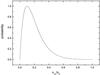 |
Fig. 4 Distribution of the initial rotation value of stars. |
The expected number of CHG between redshifts z and
z + δz can now be calculated as  (15)where Φ(L)
is the luminosity function of GRBs. We use the Schechter-function form
(15)where Φ(L)
is the luminosity function of GRBs. We use the Schechter-function form  (16)where
β = −1.12 and
L ⋆ = 9 × 1052erg s-1
(Wang & Dai 2011). The integral
(16)where
β = −1.12 and
L ⋆ = 9 × 1052erg s-1
(Wang & Dai 2011). The integral  equals
  , where Γ is the incomplete
gamma function. Because 1 + β → 0, we can approximate
, where Γ is the incomplete
gamma function. Because 1 + β → 0, we can approximate  .
.
We define an effective SFR  ,
due to the CHG, as
,
due to the CHG, as  (17)We
consider the star formation history from Hopkins & Beacom (2006),
(17)We
consider the star formation history from Hopkins & Beacom (2006),  (18)with
  .
For convenience, here we fit the data by
.
For convenience, here we fit the data by  with
α ~ 0.50. Substituting Eq. (15) into Eq. (17), we can obtain
the effective SFR as
with
α ~ 0.50. Substituting Eq. (15) into Eq. (17), we can obtain
the effective SFR as 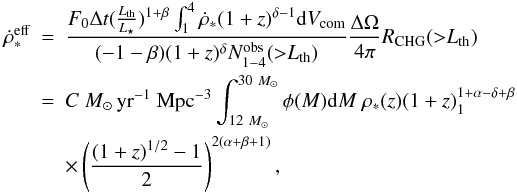 (19)where
the factor
(19)where
the factor  .
The luminosity threshold at redshift z can be calculated as
Lth = 4πDL(z)2Flim
for a given flux sensitivity Flim. For the Swift
satellite, we adopt the angular sky coverage of
ΔΩ/4π ~ 0.1, and the observation period
Δt ~ 7.5 yr. In Eq. (19),
the integral
.
The luminosity threshold at redshift z can be calculated as
Lth = 4πDL(z)2Flim
for a given flux sensitivity Flim. For the Swift
satellite, we adopt the angular sky coverage of
ΔΩ/4π ~ 0.1, and the observation period
Δt ~ 7.5 yr. In Eq. (19),
the integral  is proportional to
  . That there are many
factors in Eq. (19) may subsume the effect of changing the IMF integral for GRB production.
The evolution of
. That there are many
factors in Eq. (19) may subsume the effect of changing the IMF integral for GRB production.
The evolution of  is
shown in Fig. 3.
is
shown in Fig. 3.
Bouwens et al. (2009, 2011) measured high-redsihft SFR using color-selected Lyman break galaxies (LBGs) method. Their results are shown in Fig. 3. But LBG studies mainly probe the brightest galaxies. If the integration of UV luminosity functions decreases to MUV ≃ −10, the SFR inferred from LBG is consistent with what is derived from GRBs (Kistler et al. 2013). GRBs are found to favor sub-luminosity galaxies (Fynbo et al. 2003), so a larger fraction of the SFR within such hosts would be revealed by GRBs (Kistler et al. 2009). We can see that the SFR inferred from high-redshift GRBs can be explained well by combining Eq. (18) with Eq. (19) for C ~ 125. The overall conventional long GRB formation efficiency from massive stars is about <10-6 (Zitouni et al. 2008; Li 2008), which is lower than kCHG. This indicates that the subclass of massive stars with low metallicity and chemical homogeneity may produce long GRBs more efficiently.
5. Implications for the cosmic reionization
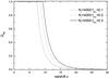 |
Fig. 5 HII filling factor QHII as a function of redshift computed for different values of fesc. |
Determining when and how the universe was reionized by early sources have been important
questions for decades (Gunn & Peterson 1965;
Robertson et al. 2010). It is established that IGM
reionization may be completed by z ≈ 6.5, based on strong
Lyα absorption from neutral hydrogen along lines of sight to quasars at
z > 6 (Fan et al. 2001). As a measure of ionization, we follow the evolution of the HII
volume-filling factor
QHII = ne/nH,
versus redshift, using the SFR derived from GRBs (Fig. 3). The average evolution of QHII is found by
numerical integration of the rate of ionizing photons minus the rate of radiative
recombinations (Madau et al. 1999; Barkana &
Loeb 2001; Wyithe & Loeb 2003; Yu et al. 2012)
 (20)Here,
  (21)is the rate
of ionizing UV photons escaping from the stars into the IGM, Nγ is the number of ionizing UV photons
released per baryon of the stars, (1 + z)3 converts the comoving
density into proper density,
is proportional to (1 + z)-3 at
z > 4.48, and fesc is
the escape fraction. The escape fraction is not well constrained. At low redshifts,
observations show that the escape fraction from GRB hosts is about a few percent (Chen
et al. 2007; Fynbo et al. 2009). But at high redshifts, the fesc is
higher (Inoue et al. 2005; Robertson et al. 2010). Recent estimates suggest that the clumping factor
C ≈ 1−6 (Bolton & Haehnelt 2007; Pawlik et al. 2009). We adopt
C = 3 in this paper. The proper density of hydrogen is
nH, and
αB = 1.63 × 10⁻¹³ cm3 s-1
is the recombination rate for an electron temperature of about 104 K. Because the
mass in collapsed objects is still low at high redshift, the IGM contains most of the
cosmological baryons, at mean density
(21)is the rate
of ionizing UV photons escaping from the stars into the IGM, Nγ is the number of ionizing UV photons
released per baryon of the stars, (1 + z)3 converts the comoving
density into proper density,
is proportional to (1 + z)-3 at
z > 4.48, and fesc is
the escape fraction. The escape fraction is not well constrained. At low redshifts,
observations show that the escape fraction from GRB hosts is about a few percent (Chen
et al. 2007; Fynbo et al. 2009). But at high redshifts, the fesc is
higher (Inoue et al. 2005; Robertson et al. 2010). Recent estimates suggest that the clumping factor
C ≈ 1−6 (Bolton & Haehnelt 2007; Pawlik et al. 2009). We adopt
C = 3 in this paper. The proper density of hydrogen is
nH, and
αB = 1.63 × 10⁻¹³ cm3 s-1
is the recombination rate for an electron temperature of about 104 K. Because the
mass in collapsed objects is still low at high redshift, the IGM contains most of the
cosmological baryons, at mean density  (22)We adopt the parameters
from WMAP seven-year data, Ωbh2 = 0.02255 ± 0.00054
and Ωmh2 = 0.1352 ± 0.0036 (Komatsu et al.
2011). The critical density is
ρcr = 1.8785 × 10⁻²⁹ h2
g cm-3. The mean hydrogen number density,
(22)We adopt the parameters
from WMAP seven-year data, Ωbh2 = 0.02255 ± 0.00054
and Ωmh2 = 0.1352 ± 0.0036 (Komatsu et al.
2011). The critical density is
ρcr = 1.8785 × 10⁻²⁹ h2
g cm-3. The mean hydrogen number density,  (23)where
Y = 0.2477 ± 0.0029 is the helium mass fraction (Peimbert et al. 2007). After the values of Nγ and fesc are
given, the evolution of the HII volume filling factor QHII can
be numerically calculated from Eq. (20). In
Fig. 5, we show the evolution
of QHII as a function of redshift. For Nγ = 4000 and
fesc = 0.2, the IGM was completely ionized at
zrei ~ 8.5.
(23)where
Y = 0.2477 ± 0.0029 is the helium mass fraction (Peimbert et al. 2007). After the values of Nγ and fesc are
given, the evolution of the HII volume filling factor QHII can
be numerically calculated from Eq. (20). In
Fig. 5, we show the evolution
of QHII as a function of redshift. For Nγ = 4000 and
fesc = 0.2, the IGM was completely ionized at
zrei ~ 8.5.
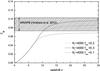 |
Fig. 6 Optical depth τe due to the scattering between the ionized gas and the CMB photons is shown. The shade region is given by the nine-year WMAP measurements (τe = 0.089 ± 0.014). The reionization history calculated from GRB-inferred SFR can easily reach τe from WMAP nine-year data. |
The cosmic microwave background (CMB) optical depth back to redshift z can
be written as the integral of
neσTdℓ, the
electron density times the Thomson cross section along proper length, ![Mathematical equation: \begin{equation} \tau_{\rm e}(z) = \int _{0}^{z} n_{\rm e}(z) \sigma_{\rm T} (1+z')^{-1} \; [c/H(z')] \; {\rm d}z' . \end{equation}](/articles/aa/full_html/2013/08/aa21623-13/aa21623-13-eq167.png) (24)After we obtain the
redshift evolution of ne(z), the CMB optical
depth as a function of redshift can then be calculated. More recently, the Planck team has
released the latest result on cosmological parameters (Planck Collaboration 2013). In the
calculation, we extrapolated the SFR as (1 + z)-3 to
z ~ 30. The first stars, so-called Population III (Pop III) stars, are
predicted to have formed at z > 20 in minihalos
(Tegmark et al. 1997; Yoshida et al. 2003). Heger et al. (2003), and Mészáros & Rees (2010)
show that Pop III stars can die as GRBs.
(24)After we obtain the
redshift evolution of ne(z), the CMB optical
depth as a function of redshift can then be calculated. More recently, the Planck team has
released the latest result on cosmological parameters (Planck Collaboration 2013). In the
calculation, we extrapolated the SFR as (1 + z)-3 to
z ~ 30. The first stars, so-called Population III (Pop III) stars, are
predicted to have formed at z > 20 in minihalos
(Tegmark et al. 1997; Yoshida et al. 2003). Heger et al. (2003), and Mészáros & Rees (2010)
show that Pop III stars can die as GRBs.
The formation rate of Pop III GRBs has been extensively studied (Campisi et al. 2011; de Souza et al. 2011). The high luminosities of GRBs make them detectable out to the edge of the
visible universe (Bromm & Loeb 2002, 2006; Wang et al. 2012), so GRBs may provide the information of SFR out to
z > 20 in future. The extrapolation of SFR to
high redshifts may be reasonable. The optical depth is shown in Fig. 6. The WMAP nine-year data gives
τe = 0.089 ± 0.014 (Hinshaw et al. 2012). The combination of Planck and WMAP data also
gives  (Planck Collaboration 2013), so our GRB-inferred SFR can reproduce the CMB optical depth.
6. Summary
Using the GRB catalogs, we have constructed the cumulative redshift distribution of 110 luminous (Liso > 1051 erg s-1) GRBs out to redshift z ~ 9.4. We find that the Swift GRBs during 2005–2012 are biased toward tracing the SFR, including a factor of about (1 + z)0.5. Correcting this evolution, we derived the star formation history up to z ~ 9.4 using Swift GRB sample. Our results show that no steep drop exists in the SFR up to at least z ~ 9.4. To explain the high-redshift GRB rate excess, the GRBs produced by rapidly rotating metal-poor stars with low mass were considered. The collapsar model explains GRB formation via the collapse of a massive star with M > 30 M⊙ into a black hole. We considered that at the low-metallicity, quasi-chemically homogeneous evolution of rapidly rotating stars with mass higher than 12 M⊙ can lead to the formation of GRBs. The low metallicity and rapid rotation can lead to efficiently produce GRBs in two ways. First, rapid rotation keeps the stars chemically homogeneous and thus avoids the formation of a massive envelope, so the stellar core is free of spin-down due to magnetic core-envelope coupling. Second, the stellar wind is weak at low metallicity, so this reduces spin-down due to stellar winds. Our fitting results confirm this idea. We also calculated the reionization history using the GRB-inferred SFR and find that this SFR can maintain cosmic reionization over 6 < z < 10 and reproduce the observed optical depth of Thomson scattering to the cosmic microwave background.
Although the lower limit mass of a star with low metallicity that can collapse to GRB is uncertain, but this value is unimportant in our analysis. The best fitting parameters will shift slightly when the lower limit mass is changed.
Acknowledgments
We thank the anonymous referee for very useful comments and suggestions. We thank K. S. Cheng and Z. G. Dai for fruitful discussions. We acknowledge the use of public data from the Swift data archive. This work is supported by the National Natural Science Foundation of China (grant 11103007 and 11033002).
References
- Barkana, R., & Loeb, A. 2001, Phys. Rep., 349, 125 [NASA ADS] [CrossRef] [Google Scholar]
- Barkana, R., & Loeb, A. 2004, ApJ, 601, 64 [NASA ADS] [CrossRef] [Google Scholar]
- Bissaldi, E., Calura, F., Matteucci, F., Longo, F., & Barbiellini, G. 2007, A&A, 471, 585 [NASA ADS] [CrossRef] [EDP Sciences] [Google Scholar]
- Bolton, J. S., & Haehnelt, M. G. 2007, MNRAS, 382, 325 [NASA ADS] [CrossRef] [Google Scholar]
- Bouwens, R. J., Illingworth, G. D., Franx, M., et al. 2009, ApJ, 705, 936 [NASA ADS] [CrossRef] [Google Scholar]
- Bouwens, R. J., Illingworth, G. D., Labbe, I., et al. 2011, Nature, 469, 504 [NASA ADS] [CrossRef] [PubMed] [Google Scholar]
- Bouwens, R. J., Illingworth, G. D., Oesch, P. A., et al. 2012, ApJ, 752, L5 [NASA ADS] [CrossRef] [Google Scholar]
- Bromm, V., & Loeb, A. 2002, ApJ, 575, 111 [NASA ADS] [CrossRef] [Google Scholar]
- Bromm, V., & Loeb, A. 2006, ApJ, 642, 382 [Google Scholar]
- Butler, N. R., Kocevski, D., Bloom, J. S., & Curtis, J. L. 2007, ApJ, 671, 656 [NASA ADS] [CrossRef] [Google Scholar]
- Butler, N. R., Bloom, J. S., & Poznanski, D. 2010, ApJ, 711, 495 [NASA ADS] [CrossRef] [Google Scholar]
- Campisi, M. A., Maio, U., Salvaterra, R., & Ciardi, B. 2011, MNRAS, 416, 2760 [NASA ADS] [CrossRef] [Google Scholar]
- Cao, X. F., Yu, Y. W., Cheng, K. S., & Zheng, X. P. 2011, MNRAS, 416, 2174 [NASA ADS] [CrossRef] [Google Scholar]
- Chen, H. W., Prochaska, J. X., & Gnedin, N. Y. 2007, ApJ, 667, L125 [NASA ADS] [CrossRef] [Google Scholar]
- Cheng, K. S., Yu, Y., & Harko, T. 2010, Phys. Rev. Lett., 104, 241102 [NASA ADS] [CrossRef] [Google Scholar]
- Ciardi, B., & Loeb, A. 2000, ApJ, 540, 687 [NASA ADS] [CrossRef] [Google Scholar]
- Coe, D., Zitrin, A., Carrasco, M., et al. 2013, ApJ, 762, 32 [NASA ADS] [CrossRef] [Google Scholar]
- Cucchiara, A., Shen, Y., Strauss, M. A., et al. 2011, ApJ, 736, 7 [NASA ADS] [CrossRef] [Google Scholar]
- Dai, Z. G., Liang, E. W., & Xu, D. 2004, ApJ, 612, L101 [NASA ADS] [CrossRef] [Google Scholar]
- de Souza, R. S., Yoshida, N., & Ioka, K. 2011, A&A, 533, A32 [NASA ADS] [CrossRef] [EDP Sciences] [Google Scholar]
- Elliott, J., Greiner, J., Khochfar, S., et al. 2012, A&A, 539, A113 [NASA ADS] [CrossRef] [EDP Sciences] [Google Scholar]
- Fan, X., Narayanan, V. K., Lupton, R. H., et al. 2001, AJ, 122, 2833 [NASA ADS] [CrossRef] [Google Scholar]
- Fruchter, A. S., Levan, A. J., Strolger, L., et al. 2006, Nature, 441, 463 [NASA ADS] [CrossRef] [PubMed] [Google Scholar]
- Fynbo, J. P. U., Jakobsson, P., Möller, P., et al. 2003, A&A, 406, L63 [NASA ADS] [CrossRef] [EDP Sciences] [Google Scholar]
- Fynbo, J. P. U., Jakobsson, P., Prochaska, J. X., et al. 2009, ApJS, 185, 526 [NASA ADS] [CrossRef] [Google Scholar]
- Gehrels, N. 1986, ApJ, 303, 336 [NASA ADS] [CrossRef] [Google Scholar]
- Gehrels, N., Ramirez-Ruiz, E., & Fox, D. B. 2009, ARA&A, 47, 567 [NASA ADS] [CrossRef] [Google Scholar]
- Gunn, J. E., & Peterson, B. A. 1965, ApJ, 142, 1633 [NASA ADS] [CrossRef] [Google Scholar]
- Heger, A., Langer, N., & Woosley, S. E. 2000, ApJ, 528, 368 [NASA ADS] [CrossRef] [Google Scholar]
- Heger, A., Fryer, C. L., Woosley, S. E., et al. 2003, ApJ, 591, 288 [NASA ADS] [CrossRef] [Google Scholar]
- Hinshaw, G., Larson, D., Komatsu, E., et al. 2012 [arXiv:1212.5226] [Google Scholar]
- Hjorth, J., Sollerman, J., Møller, P., et al. 2003, Nature, 423, 847 [NASA ADS] [CrossRef] [PubMed] [Google Scholar]
- Hopkins, A. M. 2004, ApJ, 615, 209 [NASA ADS] [CrossRef] [Google Scholar]
- Hopkins, A. M., & Beacom, J. F. 2006, ApJ, 651, 142 [NASA ADS] [CrossRef] [MathSciNet] [Google Scholar]
- Inoue, A. K., Iwata, I., Deharveng, J.-M., et al. 2005, A&A, 435, 471 [NASA ADS] [CrossRef] [EDP Sciences] [Google Scholar]
- Inoue, S., Omukai, K., & Ciardi, B. 2007, MNRAS, 380, 1715 [Google Scholar]
- Ishida, E. E. O., de Souza, R. S., & Ferrara, A. 2011, MNRAS, 418, 500 [NASA ADS] [CrossRef] [Google Scholar]
- Johnson, J. L., Dal la Vecchia, C., & Khochfa, S. 2013, MNRAS, 428, 1857 [NASA ADS] [CrossRef] [Google Scholar]
- Kewley, L., & Kobulnicky, H. A. 2007, in Island Universes: Structure and Evolution of Disc Galaxies, ed. R. S. de Jong (Dordrecht: Springer-Verlag), 435 [Google Scholar]
- Kistler, M. D., Yüksel, H., Beacom, J. F., & Stanek, K. Z. 2008, ApJ, 673, L119 [NASA ADS] [CrossRef] [Google Scholar]
- Kistler, M. D., Yüksel, H., Beacom, J. F., Hopkins, A. M., & Wyithe, J. S. B. 2009, ApJ, 705, L104 [NASA ADS] [CrossRef] [Google Scholar]
- Kistler, M. D., Yüksel, H., & Hopkins, A. M. 2013 [arXiv:1305.1630] [Google Scholar]
- Komatsu, E., Smith, K. M., Dunkley, J., et al. 2011, ApJS, 192, 18 [NASA ADS] [CrossRef] [Google Scholar]
- Lamb, D. Q., & Reichart, D. E. 2000, ApJ, 536, 1 [Google Scholar]
- Langer, N. 1998, A&A, 329, 551 [NASA ADS] [Google Scholar]
- Langer, L., & Norman, C. A. 2006, ApJ, 638, L63 [NASA ADS] [CrossRef] [Google Scholar]
- Le, T., & Dermer, C. D. 2007, ApJ, 661, 394 [NASA ADS] [CrossRef] [Google Scholar]
- Li, L. X. 2008, MNRAS, 388, 1487 [NASA ADS] [CrossRef] [Google Scholar]
- MacFadyen, A. I., Woosley, S. E., & Heger, A. 2001, ApJ, 550, 410 [NASA ADS] [CrossRef] [Google Scholar]
- Madau, P., Haardt, F., & Rees, M. J. 1999, ApJ, 514, 648 [NASA ADS] [CrossRef] [Google Scholar]
- Maeder, A., & Meynet, G. 2000, ARA&A, 38, 143 [NASA ADS] [CrossRef] [Google Scholar]
- McQuinn, M., Lidz, A., Zaldarriaga, M., et al. 2008, MNRAS, 388, 1101 [NASA ADS] [Google Scholar]
- Mészáros, P., & Ress, M. J. 2010, ApJ, 715, 967 [NASA ADS] [CrossRef] [Google Scholar]
- Mokiem, M. R., de Koter, A., Evans, C. J., et al. 2006, A&A, 456, 1131 [NASA ADS] [CrossRef] [EDP Sciences] [Google Scholar]
- Oesch, P. A., Bouwens, R. J., Illingworth, G. D., et al. 2013, ApJ, submitted [arXiv:1301.6162] [Google Scholar]
- Panter, B., Heavens, A. F., & Jimenez, R. 2004, MNRAS, 355, 764 [NASA ADS] [CrossRef] [Google Scholar]
- Pawlik, A., Schaye, J., & van Scherpenzeel, E. 2009, MNRAS, 394, 1812 [NASA ADS] [CrossRef] [Google Scholar]
- Peimbert, M., Luridiana, V., & Peimbert, A. 2007, ApJ, 666, 636 [NASA ADS] [CrossRef] [Google Scholar]
- Planck Collaboration 2013, A&A, submitted [arXiv:1303.5076] [Google Scholar]
- Porciani, C., & Madau, P. 2001, ApJ, 548, 522 [NASA ADS] [CrossRef] [Google Scholar]
- Qin, S. F., Liang, E. W., Lu, R. J., Wei, J. Y., & Zhang, S. N. 2010, MNRAS, 406, 558 [NASA ADS] [CrossRef] [Google Scholar]
- Raskin, C., Scannapieco, E., Rhoads, J., & Della Valle, M. 2008, ApJ, 689, 358 [NASA ADS] [CrossRef] [Google Scholar]
- Robertson, B. E., & Ellis, R. S. 2012, ApJ, 744, 95 [NASA ADS] [CrossRef] [Google Scholar]
- Robertson, B. E., Ellis, R. S., Dunlop, J. S., McLure, R. J., & Stark, D. P. 2010, Nature, 468, 49 [NASA ADS] [CrossRef] [PubMed] [Google Scholar]
- Salpeter, E. E. 1955, ApJ, 121, 161 [Google Scholar]
- Salvaterra, R., & Chincarini, G. 2007, ApJ, 656, L49 [NASA ADS] [CrossRef] [Google Scholar]
- Savaglio, S., 2006, New J. Phys., 8, 195 [NASA ADS] [CrossRef] [Google Scholar]
- Savaglio, S., Glazebrook, K., Le Borgne, D., et al. 2005, ApJ, 635, 260 [NASA ADS] [CrossRef] [Google Scholar]
- Schaefer, B. E. 2007, ApJ, 660, 16 [NASA ADS] [CrossRef] [Google Scholar]
- Stanek, K. Z., Matheson, T., Garnavich, P. M., et al. 2003, ApJ, 591, L17 [NASA ADS] [CrossRef] [Google Scholar]
- Svensson, K. M., Ochoa-Lara, M. T., Lovey, F., et al. 2010, MNRAS, 405, 57 [NASA ADS] [Google Scholar]
- Tanvir, N. R., Barnard, V. E., Blain, A. W., et al. 2004, MNRAS, 352, 1073 [NASA ADS] [CrossRef] [Google Scholar]
- Tegmark, M., Silk, J., Rees, M. J., et al. 1997, ApJ, 474, 1 [NASA ADS] [CrossRef] [Google Scholar]
- Thöne, C. C., Fynbo, J. P. U., Östlin, G., et al. 2008, ApJ, 676, 1151 [NASA ADS] [CrossRef] [Google Scholar]
- Totani, T. 1997, ApJ, 486, L71 [NASA ADS] [CrossRef] [Google Scholar]
- Virgili, F. J., Zhang, B., Nagamine, K., & Choi, J. H. 2011, MNRAS, 417, 3025 [NASA ADS] [CrossRef] [Google Scholar]
- Wanderman, D., & Piran, T. 2010, MNRAS, 406, 1944 [NASA ADS] [Google Scholar]
- Wang, F. Y., & Dai, Z. G. 2009, MNRAS, 400, L10 [NASA ADS] [Google Scholar]
- Wang, F. Y., & Dai, Z. G. 2011, ApJ, 727, L34 [NASA ADS] [CrossRef] [Google Scholar]
- Wang, F. Y., Qi, S., & Dai, Z. G. 2011, MNRAS, 415, 3423 [NASA ADS] [CrossRef] [Google Scholar]
- Wang, F. Y., Bromm, V., Greif, T. H. et al. 2012, ApJ, 760, 27 [NASA ADS] [CrossRef] [Google Scholar]
- Wijers, R. A. M. J., Bloom, J. S., Bagla, J. S., & Natarajan, P. 1998, MNRAS, 294, L13 [NASA ADS] [CrossRef] [Google Scholar]
- Woosley, S. E. 1993, ApJ, 405, 273 [NASA ADS] [CrossRef] [Google Scholar]
- Woosley, S. E., & Heger, A. 2006, ApJ, 643, 914 [NASA ADS] [CrossRef] [Google Scholar]
- Wyithe, J. S. B., & Loeb, A. 2003, ApJ, 586, 693 [NASA ADS] [CrossRef] [Google Scholar]
- Yoon, S. C., & Langer, L. 2005, A&A, 443, 643 [NASA ADS] [CrossRef] [EDP Sciences] [Google Scholar]
- Yoon, S. C., Langer, L., & Norman, C. 2006, A&A, 460, 199 [NASA ADS] [CrossRef] [EDP Sciences] [Google Scholar]
- Yoshida, N., Abel, T., Hernquist, L., & Sugiyama, N. 2003, ApJ, 592, 645 [NASA ADS] [CrossRef] [Google Scholar]
- Yüksel, H., Kistler, M. D., Beacom, J. F., & Hopkins, A. M. 2008, ApJ, 683, L5 [NASA ADS] [CrossRef] [Google Scholar]
- Yu, Y. W., Cheng, K. S., Chu, M. C., et al. 2012, JCAP, 07, 023 [NASA ADS] [CrossRef] [Google Scholar]
- Zitouni, H., Daigne, F., Mochkovich, R., et al. 2008, MNRAS, 386, 1597 [NASA ADS] [CrossRef] [Google Scholar]
All Figures
|
Fig. 1 Distribution of the isotropic-equivalent luminosity for 157 long-duration Swift GRBs. The GRB subsamples used to estimate the SFR are outlined. The shaded area approximates the detection threshold of Swift BAT. |
| In the text | |
|
Fig. 2 Cumulative distribution of 92 Swift GRBs with Liso > 1051 erg s-1 in z = 0−4 (stepwise solid line). The dashed line shows the GRB rate inferred from the star formation history of Hopkins & Beacom (2006). The solid line shows the GRB rate inferred from the star formation history including (1 + z)0.5 evolution. |
| In the text | |
|
Fig. 3 Cosmic star formation history. The gray points are taken from Hopkins & Beacom (2006), the dashed line shows their fitting result. The triangular points are from Bouwens et al. (2009, 2011). The open circles are taken from Robertson & Ellis (2012). The filled circles are the SFR derived from GRBs in this work. The dotted line shows the effect SFR calculated from Eq. (19). The thick solid line shows the combination of dashed and dotted lines. |
| In the text | |
|
Fig. 4 Distribution of the initial rotation value of stars. |
| In the text | |
|
Fig. 5 HII filling factor QHII as a function of redshift computed for different values of fesc. |
| In the text | |
|
Fig. 6 Optical depth τe due to the scattering between the ionized gas and the CMB photons is shown. The shade region is given by the nine-year WMAP measurements (τe = 0.089 ± 0.014). The reionization history calculated from GRB-inferred SFR can easily reach τe from WMAP nine-year data. |
| In the text | |
Current usage metrics show cumulative count of Article Views (full-text article views including HTML views, PDF and ePub downloads, according to the available data) and Abstracts Views on Vision4Press platform.
Data correspond to usage on the plateform after 2015. The current usage metrics is available 48-96 hours after online publication and is updated daily on week days.
Initial download of the metrics may take a while.