| Issue |
A&A
Volume 558, October 2013
|
|
|---|---|---|
| Article Number | A22 | |
| Number of page(s) | 6 | |
| Section | Cosmology (including clusters of galaxies) | |
| DOI | https://doi.org/10.1051/0004-6361/201321471 | |
| Published online | 30 September 2013 | |
Progenitor delay-time distribution of short gamma-ray bursts: Constraints from observations
Key Laboratory for Research in Galaxies and Cosmology CAS, Department of Astronomy, University of Science and Technology of China Hefei, Anhui 230026, PR China
e-mail: This email address is being protected from spambots. You need JavaScript enabled to view it.
Received: 14 March 2013
Accepted: 29 July 2013
Abstract
Context. The progenitors of short gamma-ray bursts (SGRBs) have not yet been well identified. The most popular model is the merger of compact object binaries (NS-NS/NS-BH). However, other progenitor models cannot be ruled out. The delay-time distribution of SGRB progenitors, which is an important property to constrain progenitor models, is still poorly understood.
Aims. We aim to better constrain the luminosity function of SGRBs and the delay-time distribution of their progenitors with newly discovered SGRBs.
Methods. We present a low-contamination sample of 16 Swift SGRBs that is better defined by a duration shorter than 0.8 s. By using this robust sample and by combining a self-consistent star formation model with various models for the distribution of time delays, the redshift distribution of SGRBs is calculated and then compared to the observational data.
Results. We find that the power-law delay distribution model is disfavored and that only the lognormal delay distribution model with the typical delay τ ≳ 3 Gyr is consistent with the data. Comparing Swift SGRBs with T90 > 0.8 s to our robust sample (T90 < 0.8 s), we find a significant difference in the time delays between these two samples.
Conclusions. Our results show that the progenitors of SGRBs are dominated by relatively long-lived systems (τ ≳ 3 Gyr), which contrasts the results found for Type Ia supernovae. We therefore conclude that primordial NS-NS systems are not favored as the dominant SGRB progenitors. Alternatively, dynamically formed NS-NS/BH and primordial NS-BH systems with average delays longer than 5 Gyr may contribute a significant fraction to the overall SGRB progenitors.
Key words: gamma-ray burst: general / binaries: close / stars: evolution / stars: formation / stars: neutron / black hole physics
© ESO, 2013
1. Introduction
Gamma-ray bursts (GRBs) are the most energetic explosions in the Universe, which can be divided into two major classes: short-duration (<2 s) bursts having a harder spectrum and long-duration (≥2 s) bursts having a softer spectrum (e.g. Nakar 2007). The bimodality of GRB duration suggests that the progenitors of these two classes are likely to be distinct. Long GRBs (LGRBs) occurring in actively star-forming galaxies with high redshift (e.g. Trentham et al. 2002) and their association with core-collapse supernovae (Hjorth et al. 2003; Woosley & Bloom 2006) suggest a strong connection between them and the collapse of massive stars (collapsars; MacFadyen & Woosley 1999), and LGRB rate is hence expected to trace the star formation rate. On the other hand, short GRBs (SGRBs) were found in elliptical galaxies (Berger et al. 2005) with very low star formation rates, demonstrating that at least some of their progenitors belong to an old stellar population (≳1 Gyr), and hence a time delay between the occurrence of the short burst and the epoch of star formation activity in their hosts is expected, implying that the progenitors of SGRBs are different from those of LGRBs. The most popular model for SGRBs is the merger of either double neutron star (NS-NS) or neutron star-black hole (NS-BH) binaries (Narayan et al. 1992). However, other possible progenitor models exist, which include accretion-induced collapse (AIC) of neutron stars (Qin et al. 1998), magnetars, and quark stars (e.g. Nakar 2007, and references therein).
The delay-time distribution of SGRB progenitors has not yet been well understood, theoretically and observationally. For the model of the merger of compact object binaries, the time delay between the formation of the two main-sequence stars and the merger of the two evolved compact objects is driven by the emission of the gravitational wave (GW), which is strongly dependent on the initial separation of the binary. A τ-1 type of delay-time distribution is a general prediction for this kind of source, as suggested by recent studies on the rate of type Ia supernovae, where the delay time is also determined by the gravitational radiation of binaries (Totani et al. 2008). Both population synthesis models (Belczynski et al. 2006) and observations of six NS-NS binaries in the Milk Way (Champion et al. 2004) support this type of delay-time distribution. On the other hand, it is also interesting to note that the mergers of low-mass BH and NS may be more common than NS-NS mergers. Bethe & Brown (1998) find that the rate of NS-BH mergers is 20 times larger than that of NS-NS mergers if the initial mass function (IMF) is supposed to be a Salpeter mass function, and the mean delay time of a NS-BH binary is ≈5 Gyr (see also Nakar 2007). It should be noticed that the above scenarios are based on primordial binaries, namely, NS-NS/BH systems that are born as binaries. Alternatively, NS-NS/BH systems can form dynamically by exchange interactions in globular clusters during their core collapse. Grindlay et al. (2006) estimate that a significant fraction (~30%) of NS-NS binaries may form by this process. The resulting delay time would be dominated by the timescale of the core-collapse of globular clusters, which is typically comparable to the Hubble time (τ ≈ 6 Gyr on average; Hopman et al. 2006). The scenario would be more complex, if there are additional populations of SGRBs. In the context of various assumptions on the delay-time distribution and cosmic star formation history with the help of the redshift distribution of the observed bursts, Nakar et al. (2006) have constrained the delay time to be longer than 4 Gyr, suggesting that primordial NS-NS progenitors are not favored. Using a combined analysis of the luminosity-redshift distribution of SGRBs and the BATSE logN-logS distribution, Virgili et al. (2011) however suggested that a significant fraction of SGRBs trace the cosmic star formation history with negligible time delays, implying that there is collapsar contamination in the SGRB population. By analyzing stellar ages and masses of the host galaxies of 19 SGRBs, Leibler & Berger (2010) found that SGRBs in early- and late-type galaxies seem to have different time delays with typical delays of ~3 Gyr and ~0.2 Gyr, respectively. It should be emphasized that most previous studies on the delay-time distribution are based on a small number of SGRBs with reliable redshift, which would seriously limit their ability to obtain a strict constraint on the luminosity function and the delay-time distribution of SGRBs.
Thanks to the Swift satellite, the sample of SGRBs with measured redshift has significantly increased over the past seven years. In this paper, we collected all Swift SGRBs with reliable redshift until 2013 June, which were selected based on the better criterion of Bromberg et al. (2013) to remove possible collapsar contamination. The luminosity function of SGRBs were then constrained using this sample. In addition, the prediction on the progenitor time delays also strongly depends on the star formation rate models. With different models on the star formation rate, the results on time delays could change significantly. Especially if the timescale of the delay is long enough (≳Gyr), the star formation at high redshifts, which often differs dramatically in different models, could play a dominate role. Here, we adopt a self-consistent method in the framework of hierarchical structure formation to construct the cosmic star formation rate (CSFR). By using this CSFR with the best-fit luminosity function, we re-examine the consistency between the observed and expected redshift distribution of SGRBs under various models for the progenitor delay-time distribution.
This paper is outlined as follows. In Sect. 2, we elaborate on the details of the star formation models we have used. In Sect. 3, we describe the method to constrain the luminosity function of SGRBs and to calculate the SGRB rate. Results are described in Sect. 4, while conclusions are summarized in Sect. 5. The cosmological parameters used in this paper are Ωm = 0.266, ΩΛ = 0.734, Ωb = 0.0449, h = 0.71, and σ8 = 0.801.
2. Model of star formation rate
We adopt a hierarchical structure formation model from Pereira & Miranda (2010), in which the CSFR is derived using the Press-Schechter (PS) like formalism. To be self-contained, we give a summary of the most important ingredients of this model in this section. Following Pereira & Miranda (2010), the equation that governs the total gas density, which includes the baryon accretion rate, the formation of stars through the transfer of baryons and the gas ejection by stars, is determined in a self-consistent way.
The evolution of the total gas density that controls the star formation history is determined by the following equation:  (1)where the first term on the right-hand side is the star formation rate, the second one is the ejected mass from stars, and the last one represents the formation of structures through the accretion of baryons from the intergalactic medium.
The accretion rate of baryons into structures is calculated as follows. In the hierarchical formation scenario, the distribution of the collapsed objects with different masses is calculated according to the simple PS formula. Throughout this paper, we adopt the Sheth-Tormen mass function (Sheth & Tormen 1999), which is a revised version of the PS mass function, given by ![Mathematical equation: \begin{eqnarray} n_{\mathrm{ST}}(M,z)\,\mathrm{d}M & = & A\sqrt{\frac{2a_{1}}{\pi}}\frac{\rho_{\mathrm{m}}}{M}\left[1+\left(\frac{\sigma^{2}}{a_{1}\delta_{\rm c}^{2}}\right)^{p}\right]\frac{\delta_{\rm c}}{\sigma}\nonumber \\ & & \times \exp\left[-\frac{a_{1}\delta_{c}^{2}}{2\sigma^{2}}\right]\frac{\mathrm{d}\ln\sigma^{-1}}{\mathrm{d}M}\,\mathrm{d}M, \end{eqnarray}](/articles/aa/full_html/2013/10/aa21471-13/aa21471-13-eq26.png) (2)where A = 0.3222, a1 = 0.707, p = 0.3, and δc = 1.686. The parameter ρm is the current mean density of the Universe, and σ is the deviation of the linear density field.
(2)where A = 0.3222, a1 = 0.707, p = 0.3, and δc = 1.686. The parameter ρm is the current mean density of the Universe, and σ is the deviation of the linear density field.
The baryon distribution is assumed to directly trace the dark matter distribution, which means that the density of baryons is just proportional to the density of dark matter by a factor. Hence, the fraction of baryons in structures at redshift z is calculated by  (3)where the threshold mass Mmin describes that stars can only form in structures that are suitably dense. Then the baryon accretion rate ab(t) that accounts for the formation of structures can be estimated by
  (4)
(4)
The star formation rate is calculated using the Schmidt law (Schmidt 1959), which gives ![Mathematical equation: \begin{equation} \frac{\mathrm{d}^{2}M_{\star}}{\mathrm{d}V\,\mathrm{d}t}=\dot{\rho}_{*}(t)=k[\rho_{\mathrm{g}}(t)]^{\alpha}, \end{equation}](/articles/aa/full_html/2013/10/aa21471-13/aa21471-13-eq38.png) (5)where k is a constant, ρg is the local gas density, and α = 1.
(5)where k is a constant, ρg is the local gas density, and α = 1.
The ejected mass from stars, which is returned to the interstellar medium, is given by  (6)where m(t) is the mass of a star that has a lifetime of t. The mass of the remnant mr depends on the progenitor mass (Pereira & Miranda 2010). The stellar IMF Φ(m) follows the standard Salpeter (1955) form, Φ(m) = Am-2.35, with a mass range of . The lifetime τm of a star with mass m is calculated using the metallicity-independent fit of Scalo (1986) and Copi (1997).
Finally, we obtain the function ρg(t) at each time t, by combing Eqs. (4), (5) and (6) with (1). Then the CSFR  , according to Eq. (5), is given by
  (7)where the constant k is given by the inverse of the timescale of star formation, namely, k = 1/τs. The CSFR is normalized to produce
  at z = 0. We use τs = 2.0 Gyr as the timescale for star formation and Mmin = 108 M⊙ for the threshold mass throughout this paper.
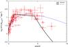 |
Fig. 1 CSFRs as a function of redshift. The dotted line represents the self-consistent model of Pereira & Miranda (2010, PM), while the solid one shows the best fit of observational data from Hopkins & Beacom (2006, HB). The observational data are taken from Hopkins (2004) (crosses) and Li (2008) (triangles). |
Figure 1 shows the CSFR as a function of redshift. We consider that the star formation begins at redshift zini = 20. As can be seen from Fig. 1, the fiducial model has an excellent agreement with the observational CSFR at redshifts z ≲ 6. An empirical fit from Hopkins & Beacom (2006, HB) is also included for comparison. Note that the self-consistent CSFR remains much flatter than the HB CSFR at redshifts z ≳ 4.5, which begins to drop exponentially.
3. Luminosity function and redshift distribution of SGRBs
3.1. Sample selection
To investigate the redshift distribution of SGRBs and thus constrain the delay-time distribution of their progenitors, we collected all Swift GRBs classified as short in the GCN circulars 1 until 2013 June, which were selected from Dietz (2011) and Kopač et al. (2012) plus GRB 100206A, GRB 111117A and GRB 130603B (J. Greiner’s web page 2 and references therein). Only GRBs with well-determined redshift and 15 to 150 keV fluence are included. According to these criteria, we obtain a list of 27 GRBs, as shown in Table 2. It is worth stressing that the classification of a GRB as a short or long burst is complicated, which depends on many factors such as duration, hardness ratio, spectral lags, etc. Most recently, Bromberg et al. (2013) argued that the Swift SGRBs that are classically selected according to these factors are heavily contaminated with collapsars and suggested that a more suitable selection for SGRBs from the Swift satellite be defined by a duration shorter than 0.8 s, which is based on a physically motivated model. To exclude any possible influence of contaminating collapsars, we adopt this better criterion and finally obtain a robust sample consisting of 16 SGRBs, which is designated as sample I. For comparison, the remaining 11 SGRBs with durations longer than 0.8 s, which have high probability to be collapsars, are considered as sample II. The redshift distributions of these two samples are shown in Fig. 2.
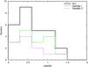 |
Fig. 2 Redshift distributions of Swift SGRBs for different samples. The solid histogram represents the full sample of 27 Swift SGRBs. The dashed and dotted histograms are for 16 SGRBs from sample I (T90 < 0.8 s) and 11 SGRBs from sample II (T90 > 0.8 s), respectively. |
3.2. Luminosity function of SGRBs
The luminosity of a GRB is computed from the isotropic equivalent energy (Eiso) and the duration of the burst containing 90% of its total energy (T90), using the standard relation:  (8)where Eiso is calculated in the energy range 1 − 104 keV in the rest-frame via a spectral shift procedure described in Bloom et al. (2001), namely,
  (9)where S is the fluence in the range of 15 − 150 keV and k(z) is the k-correction defined by
  (10)where the observed photon number spectrum N(E) can be well expressed by a Band function (Band et al. 1993). The value of k varies from 9.0 to 7.1 as the redshift increases from 0 to 3 with the peak energy Ep ~ 490 keV and low- and high-energy spectral indices α = −0.5 and β = −2.3, respectively (Nava et al. 2011). The luminosity-redshift distribution of our samples is shown in Fig. 3 with the dashed line indicating the luminosity threshold on the detector’s sensitivity:
  (11)where dL(z) is the luminosity distance, and the flux threshold Flim is taken according to the lowest luminosity of the sample, which is Flim = 5 × 10⁻⁹ erg s-1 cm-2.
Best-fit parameters of SGRB luminosity function.
List of Swift SGRBs in our sample.
The distribution of Liso then can be used to constrain the luminosity function of the SGRBs in our sample (see Fig. 3). As there is no theoretical prediction on the form of the luminosity function of SGRBs, several commonly used forms are considered, such as the broken power-laws, the Schechter functions and so on. Among them, only the lognormal function produces a reliable fitting of the data. Therefore, we use this function in this work, which reads  (12)where L0 is the mean (peak) value of the luminosity, σ is the deviation of the distribution, and Φ0 is a normalization constant. Note that no evolutionary effects of the luminosity function are considered in this work. The best-fit parameters of luminosity function for these two samples are shown in Table 1. Then we rescale these observed luminosity functions Φ(L) by the volume to which the satellite is sensitive. The obtained intrinsic luminosity function of SGRBs is as follows:
  (13)where zmax is the maximum redshift to which a GRB of luminosity L can be detected.
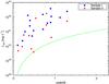 |
Fig. 3 Luminosity-redshift space of Swift SGRBs in our samples. The squares and circles represent the SGRBs from sample I and sample II, respectively. The dashed line represents the flux limit adopted in our calculation, Flim = 5 × 10⁻⁹ erg s-1 cm-2. |
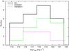 |
Fig. 4 Number distributions of the luminosities of Swift SGRBs in our samples. |
3.3. Modeling the redshift distribution of SGRBs
The SGRB rate is given by the convolution of the CSFR with the distribution of the time delays between the star formation and the occurrence of SGRBs (Piran 1992):  (14)where P(τ) is the probability distribution of the time delays τ.
Because the delay-time distribution P(τ) is not fully established theoretically, we consider the following two simple models that have been widely discussed in the literature. As mentioned previously, the studies on the rate of type Ia supernovae, whose progenitors are thought to be double-degenerate (two white dwarfs) binaries, indicate a power-law delay distribution:  (15)which also agrees with the observations of six double neutron star binaries (Champion et al. 2004) and population synthesis calculations (Belczynski et al. 2006). If the progenitors of SGRBs are dominated by primordial NS-NS binaries, then this type of delay distribution is our best-guess scenario. We note that this type of delay distribution was also adopted in the work of Guetta & Piran (2005), Nakar et al. (2006), and Virgili et al. (2011). To investigate other possibilities, we also consider a lognormal form (Nakar et al. 2006; Zheng & Ramirez-Ruiz 2007):
 ![Mathematical equation: \begin{equation} P(\tau)=\frac{\exp\{-[\ln(\tau)-\ln(\tau_{*})]^{2}/2\sigma^{2}\}}{\tau\sigma\sqrt{2\pi}}, \end{equation}](/articles/aa/full_html/2013/10/aa21471-13/aa21471-13-eq119.png) (16)with different peak values of τ∗ and a narrow (σ = 0.3) or wide (σ = 1.0) deviation. This model is useful for gaining some insight on the constraints of different timescales of delays, although it is not clear whether it is really related to the true delay distribution for compact object mergers.
(16)with different peak values of τ∗ and a narrow (σ = 0.3) or wide (σ = 1.0) deviation. This model is useful for gaining some insight on the constraints of different timescales of delays, although it is not clear whether it is really related to the true delay distribution for compact object mergers.
To compare with observations, we calculate the expected cumulative redshift distribution of the observable SGRBs for different models:  (17)where A is a constant and dV/dz is the element of the comoving volume per unit redshift, which is given by
  (18)
(18)
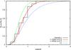 |
Fig. 5 Comparison between the observed and expected cumulative distributions of SGRBs with several representative delay-time distributions for sample I. |
4. Results
4.1. Constraints from SGRBs shorter than 0.8 s
We first consider sample I, from which SGRBs are selected according to the better criterion T90 < 0.8 s. Figure 5 shows a comparison between the cumulative redshift distributions for Swift SGRBs from sample I and the model predictions. To quantify the consistency between the observed and expected cumulative redshift distributions of SGRBs for different delay distribution models, an one-sample Kolmogorov-Smirnov (K-S) test is used. When assuming that the delay-time distribution is described as a power-law of τ-1, we find a K-S probability of only 0.04, indicating that this delay distribution model is disfavored by the observational data. This is different from the results found for Type Ia supernovae, which agrees with previous analyses (e.g. Nakar et al. 2006; Zheng & Ramirez-Ruiz 2007; Gal-Yam et al. 2008; Guetta & Stella 2009; Virgili et al. 2011). For a narrow lognormal delay distribution, we find that the most likely delay is τ∗ = 5.7 Gyr (P ≈ 0.71), and its P > 0.05 interval is 3.2 Gyr < τ∗ < 7.7 Gyr. While under the assumption of a wide lognormal delay distribution, the most likely delay is longer than the Hubble time, and its P > 0.05 interval is τ∗ > 1.9 Gyr.
Given the observational uncertainty in the CSFR at high redshifts, we repeat our analysis by using the HB CSFR. As shown in Fig. 1, the HB CSFR falls exponentially at redshifts z ≳ 4.5. The results obtained with this CSFR are similar to those obtained by using the self-consistent CSFR. For instance, we find that the most likely delay, when considering a narrow lognormal delay distribution with HB CSFR, is τ∗ = 4.6 Gyr (P ≈ 0.75), and its P > 0.05 interval is 2.3 Gyr < τ∗ < 6.6 Gyr. It is worth mentioning that the typical delay time we obtained is also smaller with the smaller star formation rate at high redshifts. With a better understanding of the distribution of time delays, this implies that the SGRB rate could also be used to constrain the star formation at high redshifts in the future.
4.2. Comparison with SGRBs longer than 0.8 s
As pointed out in Sect. 3.1 at the suggestion of Bromberg et al. (2013), there is a high probability that the physical origin of Swift SGRBs from sample II with T90 > 0.8 s is different from that of Swift SGRBs from sample I with T90 < 0.8 s, which could lead to a difference in their delay-time distributions. To check if these two samples show any significant difference in their delay-time distributions, we repeat our analysis for sample II. The comparison of the redshift distribution of the observed SGRBs from sample II with the model predictions is shown in Fig. 6. For sample II, the power-law (τ-1) delay distribution model is fully consistent with the data (P ≈ 0.69), in contrast to what is found in sample I. Under the assumption of the narrow lognormal delay distribution, the most likely delay is τ∗ = 4.7 Gyr, and the P > 0.05 interval is τ∗ < 11.7 Gyr, which implies that the progenitors of these SGRBs from sample II are younger than those from sample I. The difference in the delay-time distribution between these two samples could be the result of the collapsar contamination in the sample of SGRBs with T90 > 0.8 s or, alternatively, the existence of additional populations.
5. Conclusions and discussions
The delay-time distribution of SGRBs is an important property to single out viable progenitor models. We presented here a robust sample of 16 SGRBs with reliable redshift and 15 to 150 keV fluence, which were discovered by the Swift satellite until 2013 June. These SGRBs in our sample are selected according to a better criterion (T90 < 0.8 s) suggested by Bromberg et al. (2013), which could eliminate a very substantial contamination of collapsar GRBs. Based on this robust sample of Swift SGRBs in the context of various models for the progenitor delay-time distribution and a self-consistent CSFR, we re-examined whether the model predictions of the redshift distribution of SGRBs are consistent with the observational data. For this better sample of Swift SGRBs with T90 < 0.8 s, we find that the model with a power-law delay distribution of τ-1 shows little consistency with the observational data, in contrast to the results found for Type Ia supernovae, which agrees with previous studies (Nakar et al. 2006; Zheng & Ramirez-Ruiz 2007; Gal-Yam et al. 2008; Virgili et al. 2011). We therefore conclude that primordial NS-NS systems are disfavored as the dominant SGRB progenitors. When considering a model with a narrow lognormal delay distribution, we find that the most likely delay is τ∗ ~ 5.7 Gyr, and the typical delay is τ∗ > 3.2 Gyr at a 95% confidence level, which is relatively shorter than the results of previous analyses that proposed delays longer than ~6 − 7 Gyr (e.g. Nakar et al. 2006; Zheng & Ramirez-Ruiz 2007). This result implies that the progenitors of SGRBs are dominated by long-lived systems (τ ≳ 3 Gyr), which could be understood if dynamically formed NS-NS/BH systems with an average delay of ≈6 Gyr (Hopman et al. 2006) contribute a significant fraction to the total number of SGRBs, as proposed by Salvaterra et al. (2008), Guetta & Stella (2009) and Lee et al. (2010). Another possible candidate could be primordial NS-BH systems if these systems do indeed have an average delay of ≈5 Gyr (see Bethe & Brown 1998; Nakar 2007).
We also tested whether there is any difference between Swift SGRBs with T90 < 0.8 s and those with T90 > 0.8 s, which is expected if the Swift SGRBs with T90 > 0.8 s are heavily contaminated by collapsars. We find that Swift SGRBs from the T90 > 0.8 s sample have shorter delays than those with T90 < 0.8 s, which could be interpreted as the contamination by collapsars, as suggested by Virgili et al. (2011) and Bromberg et al. (2013). However, the possibility of the existence of additional populations cannot be excluded. We caution that a more detailed comparison of the host galaxies of Swift SGRBs with T90 > 0.8 s to those of LGRBs is needed before any firm conclusion can be drawn, as also suggested by Leibler & Berger (2010).
Although the sample of Swift SGRBs with reliable redshift has significantly expanded in the past seven years, their total number is still small, which prohibits a strict constraint on their luminosity function and delay-time distribution. The importance of the contribution of dynamically formed NS-NS systems and NS-BH systems would only be severely
constrained by the detection of more high-redshift (z > 1) SGRBs. Detailed observations of the host galaxies of individual SGRB are also essential to provide a better description of the distribution of time delays. Because these merging binary systems are also one of the most powerful sources of GWs, it is expected that the detection of GW signals from these sources would be helpful for validating different theoretical models. In particular, it would be relatively easy for a GW detector to distinguish between these two type of sources and then to constrain their relative contribution to the occurrence of SGRBs, models, since NS-BH mergers emit more powerful and lower frequency GWs than NS-NS mergers.
Acknowledgments
We thank the anonymous referee for her/his useful suggestions, which have significantly improved this paper. We also thank J. Greiner for his online GRB Table. This work is partially supported by National Basic Research Program of China (2009CB824800, 2012CB821800), the National Natural Science Foundation (11073020, 11133005, 11233003), and the Fundamental Research Funds for the Central Universities (WK2030220004).
References
- Band, D., Matteson, J., Ford, L., et al. 1993, ApJ, 413, 281 [NASA ADS] [CrossRef] [Google Scholar]
- Belczynski, K., Perna, R., Bulik, T., et al. 2006, ApJ, 648, 1110 [NASA ADS] [CrossRef] [Google Scholar]
- Berger, E., Price, P. A., Cenko, S. B., et al. 2005, Nature, 438, 988 [NASA ADS] [CrossRef] [PubMed] [Google Scholar]
- Bethe, H. A., & Brown, G. E. 1998, ApJ, 506, 780 [NASA ADS] [CrossRef] [Google Scholar]
- Bloom, J. S., Frail, D. A., & Sari, R. 2001, AJ, 121, 2879 [NASA ADS] [CrossRef] [Google Scholar]
- Bromberg, O., Nakar, E., Piran, T., & Sari, R. 2013, ApJ, 764, 179 [NASA ADS] [CrossRef] [Google Scholar]
- Champion, D. J., Lorimer, D. R., McLaughlin, M. A., et al. 2004, MNRAS, 350, L61 [NASA ADS] [CrossRef] [Google Scholar]
- Copi, C. J. 1997, ApJ, 487, 704 [NASA ADS] [CrossRef] [Google Scholar]
- Dietz, A. 2011, A&A, 529, A97 [NASA ADS] [CrossRef] [EDP Sciences] [Google Scholar]
- Gal-Yam, A., Nakar, E., Ofek, E. O., et al. 2008, ApJ, 686, 408 [NASA ADS] [CrossRef] [Google Scholar]
- Grindlay, J., Portegies Zwart, S., & McMillan, S. 2006, Nature Phys., 2, 116 [Google Scholar]
- Guetta, D., & Piran, T. 2005, A&A, 435, 421 [Google Scholar]
- Guetta, D., & Stella, L. 2009, A&A, 498, 329 [NASA ADS] [CrossRef] [EDP Sciences] [Google Scholar]
- Hjorth, J., Sollerman, J., Møller, P., et al. 2003, Nature, 423, 847 [NASA ADS] [CrossRef] [PubMed] [Google Scholar]
- Hopkins, A. M. 2004, ApJ, 615, 209 [NASA ADS] [CrossRef] [Google Scholar]
- Hopkins, A. M., & Beacom, J. F. 2006, ApJ, 651, 142 [NASA ADS] [CrossRef] [MathSciNet] [Google Scholar]
- Hopman, C., Guetta, D., Waxman, E., & Portegies Zwart, S. 2006, ApJ, 643, L91 [NASA ADS] [CrossRef] [Google Scholar]
- Kopač, D., D’Avanzo, P., Melandri, A., et al. 2012, MNRAS, 424, 2392 [NASA ADS] [CrossRef] [Google Scholar]
- Lee, W. H., Ramirez-Ruiz, E., & van de Ven, G. 2010, ApJ, 720, 953 [NASA ADS] [CrossRef] [Google Scholar]
- Leibler, C. N., & Berger, E. 2010, ApJ, 725, 1202 [NASA ADS] [CrossRef] [Google Scholar]
- Li, L.-X. 2008, MNRAS, 388, 1487 [NASA ADS] [CrossRef] [Google Scholar]
- MacFadyen, A. I., & Woosley, S. E. 1999, ApJ, 524, 262 [NASA ADS] [CrossRef] [Google Scholar]
- Nakar, E. 2007, Phys. Rep., 442, 166 [NASA ADS] [CrossRef] [Google Scholar]
- Nakar, E., Gal-Yam, A., & Fox, D. B. 2006, ApJ, 650, 281 [NASA ADS] [CrossRef] [Google Scholar]
- Narayan, R., Paczynski, B., & Piran, T. 1992, ApJ, 395, L83 [NASA ADS] [CrossRef] [Google Scholar]
- Nava, L., Ghirlanda, G., Ghisellini, G., & Celotti, A. 2011, A&A, 530, A21 [NASA ADS] [CrossRef] [EDP Sciences] [Google Scholar]
- Pereira, E. S., & Miranda, O. D. 2010, MNRAS, 401, 1924 [NASA ADS] [CrossRef] [Google Scholar]
- Piran, T. 1992, ApJ, 389, L45 [NASA ADS] [CrossRef] [Google Scholar]
- Qin, B., Wu, X.-P., Chu, M.-C., Fang, L.-Z., & Hu, J.-Y. 1998, ApJ, 494, L57 [NASA ADS] [CrossRef] [Google Scholar]
- Salpeter, E. E. 1955, ApJ, 121, 161 [Google Scholar]
- Salvaterra, R., Cerutti, A., Chincarini, G., et al. 2008, MNRAS, 388, L6 [NASA ADS] [Google Scholar]
- Scalo, J. M. 1986, Fund. Cosmic Phys., 11, 1 [NASA ADS] [EDP Sciences] [Google Scholar]
- Schmidt, M. 1959, ApJ, 129, 243 [NASA ADS] [CrossRef] [Google Scholar]
- Sheth, R. K., & Tormen, G. 1999, MNRAS, 308, 119 [NASA ADS] [CrossRef] [Google Scholar]
- Totani, T., Morokuma, T., Oda, T., Doi, M., & Yasuda, N. 2008, PASJ, 60, 1327 [NASA ADS] [CrossRef] [Google Scholar]
- Trentham, N., Ramirez-Ruiz, E., & Blain, A. W. 2002, MNRAS, 334, 983 [NASA ADS] [CrossRef] [Google Scholar]
- Virgili, F. J., Zhang, B., O’Brien, P., & Troja, E. 2011, ApJ, 727, 109 [NASA ADS] [CrossRef] [Google Scholar]
- Woosley, S. E., & Bloom, J. S. 2006, ARA&A, 44, 507 [NASA ADS] [CrossRef] [Google Scholar]
- Zheng, Z., & Ramirez-Ruiz, E. 2007, ApJ, 665, 1220 [NASA ADS] [CrossRef] [Google Scholar]
All Tables
All Figures
|
Fig. 1 CSFRs as a function of redshift. The dotted line represents the self-consistent model of Pereira & Miranda (2010, PM), while the solid one shows the best fit of observational data from Hopkins & Beacom (2006, HB). The observational data are taken from Hopkins (2004) (crosses) and Li (2008) (triangles). |
| In the text | |
|
Fig. 2 Redshift distributions of Swift SGRBs for different samples. The solid histogram represents the full sample of 27 Swift SGRBs. The dashed and dotted histograms are for 16 SGRBs from sample I (T90 < 0.8 s) and 11 SGRBs from sample II (T90 > 0.8 s), respectively. |
| In the text | |
|
Fig. 3 Luminosity-redshift space of Swift SGRBs in our samples. The squares and circles represent the SGRBs from sample I and sample II, respectively. The dashed line represents the flux limit adopted in our calculation, Flim = 5 × 10⁻⁹ erg s-1 cm-2. |
| In the text | |
|
Fig. 4 Number distributions of the luminosities of Swift SGRBs in our samples. |
| In the text | |
|
Fig. 5 Comparison between the observed and expected cumulative distributions of SGRBs with several representative delay-time distributions for sample I. |
| In the text | |
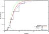 |
Fig. 6 Same as Fig. 5, but for Swift SGRBs from sample II. |
| In the text | |
Current usage metrics show cumulative count of Article Views (full-text article views including HTML views, PDF and ePub downloads, according to the available data) and Abstracts Views on Vision4Press platform.
Data correspond to usage on the plateform after 2015. The current usage metrics is available 48-96 hours after online publication and is updated daily on week days.
Initial download of the metrics may take a while.