| Issue |
A&A
Volume 555, July 2013
|
|
|---|---|---|
| Article Number | A118 | |
| Number of page(s) | 11 | |
| Section | Planets and planetary systems | |
| DOI | https://doi.org/10.1051/0004-6361/201321462 | |
| Published online | 10 July 2013 | |
Transiting exoplanets from the CoRoT space mission⋆
XXIV. CoRoT-25b and CoRoT-26b: two low-density giant planets
1 Aix Marseille Université, CNRS, LAM (Laboratoire d’Astrophysique de Marseille) UMR 7326, 13388 Marseille, France
e-mail: This email address is being protected from spambots. You need JavaScript enabled to view it.
2 Institut d’Astrophysique de Paris, 98bis boulevard Arago, 75014 Paris, France
3 Department of Astronomy, New Mexico State University, PO Box 30001, MSC 4500, Las Cruces, NM 88003-8001, USA
4 NASA Postdoctoral Program Fellow, Ames Research Center, PO Box 1, Moffett Field, CA 94035, USA
5 Research and Scientific Support Department, ESTEC/ESA, PO Box 299, 2200 AG Noordwijk, The Netherlands
6 Instituto de Astrofisica de Canarias, 38205 La Laguna, Tenerife, Spain
7 Universidad de La Laguna, Dept. de Astrofísica, 38200 La Laguna, Tenerife, Spain
8 Thüringer Landessternwarte, Sternwarte 5, Tautenburg 5, 07778 Tautenburg, Germany
9 Observatoire de la Côte d’Azur, Laboratoire Cassiopée, BP 4229, 06304 Nice Cedex 4, France
10 Institute of Planetary Research, German Aerospace Center, Rutherfordstrasse 2, 12489 Berlin, Germany
11 Department of Physics, Denys Wilkinson Building Keble Road, Oxford, OX1 3RH, UK
12 Observatoire de l’Université de Genève, 51 chemin des Maillettes, 1290 Sauverny, Switzerland
13 LESIA, Obs de Paris, Place J. Janssen, 92195 Meudon Cedex, France
14 INAF − Osservatorio Astronomico di Torino, via Osservatorio 20, 10025 Pino Torinese, Italy
15 Institut d’astrophysique spatiale, Université Paris-Sud 11 & CNRS, UMR 8617, Bât. 121, 91405 Orsay, France
16 McDonald Observatory, The University of Texas at Austin, Austin, TX 78712, USA
17 University of Vienna, Institute of Astronomy, Türkenschanzstr. 17, 1180 Vienna, Austria
18 IAG, Universidade de Sao Paulo, Brazil
19 Observatoire de Haute Provence, 04670 Saint Michel l’ Observatoire, France
20 University of Liège, Allée du 6 août 17, Sart Tilman, Liège 1, Belgium
21 Space Research Institute, Austrian Academy of Science, Schmiedlstr. 6, 8042 Graz, Austria
22 Wise Observatory, Tel Aviv University, 69978 Tel Aviv, Israel
23 Institut für Astrophysik, Georg-August-Universität, Friedrich-Hund-Platz 1, 37077 Göttingen, Germany
24 Rheinisches Institut für Umweltforschung an der Universität zu Köln, Aachener Strasse 209, 50931 Köln, Germany
25 Center for Astronomy and Astrophysics, TU Berlin, Hardenbergstr. 36, 10623 Berlin, Germany
26 LUTH, Observatoire de Paris, CNRS, Université Paris Diderot, 5 place Jules Janssen, 92195 Meudon, France
27 Department of Physics and Astronomy, Aarhus University, 8000 Aarhus C, Denmark
Received: 13 March 2013
Accepted: 24 May 2013
Abstract
We report the discovery of two transiting exoplanets, CoRoT-25b and CoRoT-26b, both of low density, one of which is in the Saturn mass-regime. For each star, ground-based complementary observations through optical photometry and radial velocity measurements secured the planetary nature of the transiting body and allowed us to fully characterize them. For CoRoT-25b we found a planetary mass of 0.27 ± 0.04 MJup, a radius of 1.08-0.10+0.3 RJup and hence a mean density of 0.15-0.06+0.15 g cm-3. The planet orbits an F9 main-sequence star in a 4.86-day period, that has a V magnitude of 15.0, solar metallicity, and an age of 4.5-2.0+1.8-Gyr. CoRoT-26b orbits a slightly evolved G5 star of 9.06 ± 1.5-Gyr age in a 4.20-day period that hassolar metallicity and a V magnitude of 15.8. With a mass of 0.52 ± 0.05 MJup, a radius of 1.26-0.07+0.13 RJup, and a mean density of 0.28-0.07+0.09 g cm-3, it belongs to the low-mass hot-Jupiter population. Planetary evolution models allowed us to estimate a core mass of a few tens of Earth mass for the two planets with heavy-element mass fractions of 0.52-0.15+0.08 and 0.26-0.08+0.05, respectively, assuming that a small fraction of the incoming flux is dissipated at the center of the planet. In addition, these models indicate that CoRoT-26b is anomalously large compared with what standard models could account for, indicating that dissipation from stellar heating could cause this size.
Key words: planetary systems / techniques: photometric / techniques: radial velocities / techniques: spectroscopic
The CoRoT space mission, launched on December 27th 2006, has been developed and is operated by CNES, with the contribution of Austria, Belgium, Brazil, ESA (RSSD and Science Programme), Germany and Spain. Partly based on observations obtained at the European Southern Observatory at Paranal and La Silla, Chile in programs 083.C-0690(A), 184.C-0639.
© ESO, 2013
1. Introduction
More than 190 giant exoplanets (mass and radius larger than 0.1 MJup, 0.5 RJup) transiting their parent stars have been discovered, mostly with dedicated photometric surveys, such as TrES (Alonso et al. 2004), WASP (Pollacco et al. 2006), and HAT (Bakos et al. 2007) from the ground, and CoRoT and Kepler from space (Baglin et al. 2009; Borucki et al. 2010). Transiting planets constitute a unique testbed for precise modeling of exoplanet structure and evolution, because the combination of photometric and spectrometric measurements can lead to the accurate determination of the physical and orbital properties of the planets and their host stars. This well-characterized planet population allows one to probe their internal structure and furthermore provides some hints on the physical processes that occur in their interior (e.g. Laughlin et al. 2011). While the number of transiting planets in the Jupiter and higher mass regime has increased to more than one hundred mostly well-characterized members, planets in the Saturn mass domain (0.1−0.4 MJup) remain rare; there are currently only 18 with masses between 0.1 and 0.4 MJupand sizes larger than 0.5 RJup . We still need to better assess how the properties of these two classes of the giant close-in population compare and whether the same formation mechanisms occur in both.
We report the discovery of CoRoT-25b and CoRoT-26b, which belong to the low-mass range of the giant close-in population. In Sect. 2, we present the CoRoT observations and in Sect. 3, the ground-based follow-up observations that were used to confirm the planetary nature of the objects and determined their masses. In Sect. 4, we describe the spectral analysis that leads to the determination of the host stars’ fundamental parameters, surface gravity, effective temperature, and abundances. The orbital and physical parameters of the planets are then derived with a global fitting method that combines photometric and radial velocity measurements (Sect. 5). The properties of these two planets have been explored with two different approaches based on evolution models, and the results are presented in Sect. 6. We conclude in Sect. 7 with a brief comparison of these two planets with the giant population.
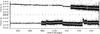 |
Fig. 1 CoRoT light curve from raw data of CoRoT-25 (top) and CoRoT-26 (bottom). The changes in sampling rates from 512 to 32 s appear as increases in the scatter. In gray dots, the 32 s integrations are binned to 512 s. The light curves show discontinuities due to the impact of high-energy particles and other instrumental effects. The transits can be seen as regular dips. |
2. CoRoT observations
The CoRoT observation run LRc02 corresponds to a 145-day run from April 14 to September 7, 2008 in the Galactic center direction. Three more planets have previously been reported from this run: CoRoT-6b (Fridlund et al. 2010), CoRoT-9b (Deeg et al. 2010), and CoRoT-11b (Gandolfi et al. 2010).
The first transits of CoRoT-25b and CoRoT-26b were detected 99 and 51 days after the begining of the run by the Alarm Mode (Surace et al. 2008; Bonomo et al. 2012), in the monochromatic light curves (see Fig. 1) of the targets LRc02_E1_1280 and LRc02_E2_4747, respectively. After the initial detection, the sampling rate of both targets was switched from 512 s to 32 s. The transits of CoRoT-25b and CoRoT-26b were identified with an orbital period of 4.9 and 4.2 days, and both have a transit depth of ≈0.5% (contaminated values). Coordinates, identifications, magnitudes, and additional parameters are given in Table 3.
Factors for photometric contamination of the targets’ flux from nearby stars were computed for each CoRoT aperture mask (Fig. 2) with two methods. We first used the approach developed by Pasternacki et al. (2011), which consists of modeling the point spread function (PSF) of the target and contaminating stars and of calculating its flux contribution in the photometric aperture. Contamination factors of 1.3 ± 0.3% and 10.9 ± 0.9% for CoRoT-25 and CoRoT-26 are obtained. Second, we applied the method from Gardes et al. (2011), which is conceptually similar to the previous one, but found contaminations of 3.4 ± 0.9% and 10.4 ± 1.2%. Results from the two methods agree for CoRoT-26, but differ by two sigmas for CoRoT-25. The difference in the contamination estimates arises from possible differences in recentering the stellar PSF model on the photometric mask, because CoRoT does not provide individual images for each exposure. Finally, we decided to adopt weighted mean values from both methods, that is, 1.8 ± 0.3% for CoRoT-25 and 10.7 ± 0.7% for CoRoT-26. In both cases, the errors of the contamination factors (which affect the relative depth of the transits) are too small to contribute significantly to the final system parameter errors reported in Table 3.
CoRoT light curves were processed with the CoRoT Data Analysis pipeline, which removes signatures in the light curves that are correlated with systematic error sources from the telescope and spacecraft, such as pointing drift, focus change, and flag features due to high-energy-particle impact, and thermal transients (Drummond et al. 2006; Auvergne 2006; Drummond et al. 2008). The remaining jumps and discontinuities were corrected. For the analysis, we kept only the light curves covering a span of 2.4 h for CoRoT-25 and 8.2 h for CoRoT-26 before and after each transit, corrected for the contamination, and binned the data sampled with the 32 s rate those sampled with 512 s. In addition, we removed some remaining low-frequency modulations by subtracting a parabolic fit of the off-transit data and normalized the light curves, as has generally been performed for CoRoT planet detections (e.g. Alonso et al. 2008).
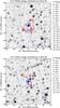 |
Fig. 2 POSS image of CoRoT-25 and CoRoT-26 (marked with a red cross in the center of the field) with the CoRoT mask superimposed (in blue solid line), and the contaminating stars (red crosses identified with a number, the contaminating R-magnitude its at the right of the image). |
3. Ground-based follow-up observations
3.1. Photometric measurements
The main objective of ground-based photometric follow-up is to check whether the observed transit features occur on the target star and not on a potential background eclipsing-binary system (Deeg et al. 2009). Following-up CoRoT exoplanetary candidates is challenging because of the faintness of the targets and the need for time-critical observations, given the transit ephemeris. For this reason, the photometric follow-up of the candidate CoRoT-25b was performed with three telescopes. Observations with short on- and off-transit coverages were acquired on June 6, 2010 with the Canada France Hawaii Telescope (CFHT), and on June 11, 2010 with the 1.2-m Euler telescope at La Silla Observatory. Both indicated a detection of the transit on the target star, but because of timing errors from ephemeris uncertainties, we did not consider this result as sufficiently reliable. Longer coverage of a full transit was obtained on June 15, 2010 with the IAC80 telescope at the Teide Observatory, which confirmed that the transits occur on the target star, with a depth of about 0.5%. Nearby eclipsing binaries, at distances larger than ~1.5′′ from the target, could therefore be excluded as a source of a false positive.
Photometric follow-up observations of CoRoT-26b were performed in July and August 2008 with both the IAC80 and 1.2-m Euler telescopes. The runs consisted of short on-off observations in and out of transits. The observations from the IAC80 were unable to detect the transit in the target star, but their quality in combination with a smaller timing error was sufficient to exclude that CoRoT’s signal could arise from any nearby contaminator. Then, the Euler observations showed a clear transit on the target with a depth of 0.8 ± 0.3%, fully compatible with the photometric dimming measured by CoRoT and rejecting that any eclipsing binary at distances larger than ~1.5′′ from the target may have caused a false alarm.
3.2. Spectroscopic and radial velocity measurements
Radial velocity (RV) measurements were performed with the HARPS spectrometer at the focus of ESO’s 3.6-m telescope at La Silla, as part of the ESO large program 184.C-0639. Some observations were also obtained with HIRES on the 10-m Keck-1 telescope, as part of a NASA key science project to support the CoRoT mission. HARPS was used with the observing mode obj_AB, without simultaneous thorium calibration to monitor the Moon background light on its second fiber. The exposure time was set to one hour. We reduced the HARPS data and computed the RVs with a pipeline based on the cross-correlation techniques (Baranne et al. 1996; Pepe et al. 2002). Radial velocities were obtained by weighted cross-correlation with a numerical G2 mask. For some exposures contaminated by moonlight, we made the correction described by Bonomo et al. (2010), which consist of substracting the cross-correlation function (CCF) from the second fibre, which contains the Sun spectrum (reflected by the Moon), from the stellar CCF. HIRES observations were performed with the red cross-disperser and the I2-cell to measure RVs. We used the 0.861-arcsec wide slit that leads to a resolving power of R ≈ 45 000. Differential radial velocities were computed using the Austral Doppler code (Endl et al. 2000).
3.2.1. Radial velocities of CoRoT-25
A set of 28 spectra was recorded for CoRoT-25 with HARPS between September 9, 2009 and September 22, 2011, including nine consecutive exposures of twice one hour made during one night. The signal-to-noise ratio (S/N) per pixel at 550 nm ranges from 5 to 14. Five measurements were slightly affected by the moonlight. The correction provided by the substraction of the Moon CCF from the stellar CCF induced an RV change of up to 76 m s-1for these five measurements. A set of six exposures was recorded with HIRES on June 29−30, 2009 and on July 23−24, 2011, including two consecutive exposures of twice one hour made during one night without Moon contamination.
Radial velocity measurements of CoRoT-25 obtained with HARPS and HIRES.
The HARPS and HIRES radial velocities are given in Table 1. The two sets of relative radial velocities were simultaneously fitted with a Keplerian model, where the transit epoch and period are fixed at values from a first modeling of the CoRoT light curve, and where an offset was adjusted between the two different instruments. No significant eccentricity was found, and we decided hereafter to set it to zero. The best solution is obtained for a semi-amplitude K = 30.0 ± 4.6 m s-1and an offset for the HIRES radial velocities of −15.4185 ± 0.007 km s-1. The dispersion of the residuals is 25 m s-1and the reduced χ2 is 1.1. We also computed the average of each double measurement (obtained during the same night) and found a very similar result with K = 31.6 ± 3.9 m s-1and a residual dispersion of 10 m s-1. The joint analysis of the photometric and RV data in Sect. 5 does not change these results. Figure 3 shows all RV measuremens after subtracting the RV offset and a phase-folding to the orbital period.
To examine the possibility that the RV variation is due to a blended-binary scenario – a single star plus an unresolved eclipsing binary –, we followed the procedure described in Bouchy et al. (2009b). It consists of checking the spectral line asymmetries and the dependance of the RV variations as a function of the cross-correlation mask (a template spectrum made of box-shaped emission lines at the position of selected spectral lines for a specific spectral type − see Baranne et al. 1996). To increase the S/N of the cross-correlation function (CCF) bisectors, we averaged the CCFs close to the same orbital phase φ, at φ = 0.25 and φ = 0.75. Sixteen and 11 CCFs were averaged with orbital phases in the ranges of 0.1−0.4 and 0.6−0.9, respectively. The bisectors were computed on these two averaged CCFs; no significant variation of the bisector span was observed (Fig. 4). Furthermore, the radial velocities were computed with different cross-correlation templates (F0, G2, and K5) without a significant change in the amplitude of the RV variations. These two checks exclude some configurations of blended binaries, which supports the planetary nature of CoRoT-25b.
No significant radial velocity drift (<100 m/s) was detected during the two years covered by the HARPS and HIRES measurements. This excludes the presence of any other massive giant planet (>5 MJup) at closer than 3 AU in the system.
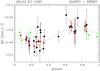 |
Fig. 3 Phase-folded radial velocities of CoRoT-25. The black circles and green squares correspond to HARPS and HIRES measurements. The red open circles correspond to the averages of the double (same night) measurements. |
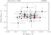 |
Fig. 4 HARPS bisector span versus radial velocities of CoRoT-25. The two red circles correspond to the averaged cross-correlation functions at the extreme phases of φ = 0.25 and 0.75. |
3.2.2. Radial velocities of CoRoT-26
A set of 27 spectra was recorded for CoRoT-26 with HARPS between July 10, 2009 and September 23, 2011, including seven consecutive exposures of twice one hour made during one night (Table 2). Three measurements with a S/N (per pixel at 550 nm) lower than 4 were rejected. The remaining 24 measurements, listed in Table 2, have an S/N from 4 to 8. The first measurement was slightly affected by moonlight, but the RV of the Moon was far away from the stellar RV and did not require correction. The fourth measurement was affected by the Moon, with its RV close to the stellar one. The correction induced a change of 225 m s-1for this exposure. All other measurements were made during dark time. We fitted the dataset with a Keplerian model, where the transit epoch and period are fixed at values from a first modeling of the CoRoT light curve. No significant eccentricity was detected, and hereafter it was set it to zero. The best solution is obtained for a semi-amplitude K = 56.9 ± 8.4 m s-1. The dispersion of the residuals is 35 m s-1and the reduced χ2 is 0.98. We also computed the mean of each double measurement (obtained during the same night) and obtained K = 64.5 ± 11 m s-1compatible within 1σ to the previous determination and a residual dispersion of 20 m s-1. The posterior joint analysis of the photometric and RV data did not change these results within error bars. In Fig. 5, we plot the radial velocity measurements phase-folded to the orbital period.
To examine whether the radial velocity variation could be caused by a diluted eclipsing binary, we averaged the CCFs close to the same extreme phases. Five and seven CCFs were averaged at orbital phases in the ranges 0.2−0.3 and 0.7−0.8. Bisector spans were computed on these two averaged CCFs, but showed no significant variations (Fig. 6). Furthermore, the radial velocities were computed with different cross-correlation templates (F0, G2 and K5) without a significant change in the amplitude of the RV variations. These two checks exclude some configurations of a blended binary, which supports the planetary nature of CoRoT-26b.
No significant RV drift (<200 m/s) was found over the two years of HARPS data, excluding any additional massive sub-stellar companion (>10 MJup) at closer than 3 AU in the system.
Radial velocity measurements of CoRoT-26 obtained with HARPS.
4. Stellar parameters and interstellar extinction
We obtained a spectrum of CoRoT-25 with UVES/VLT using the 390 + 580 nm setting, which covers the wavelength range from 327.4 to 450.6 nm and 478.5 to 681.7 nm. With the slit-width of 0.8 arcsec, the spectrum has a resolution λ/Δλ ~ 50 000. Three spectra were taken in service mode (program 083.C-0690(A)) on September 25, 2010, September 28, 2010, and September 29, 2010, each exposed for one hour. We used IRAF routines to remove the bias offset, to flat-field the data, to remove cosmic ray hits, and to extract and wavelength-calibrate the spectrum. The three spectra, set in the rest frame, were then co-added and used to derive a first estimate of the spectral type of the host star and to confirm that it is a dwarf-type star. We then took advantage of the HARPS spectra that were collected for the RV analysis, because they provide a higher spectral resolution. These spectra, once set in the rest frame, were co-added following the methodology described for previous CoRoT planets (e.g. Rauer et al. 2009) and produced spectra with a typical S/N of 230 for CoRoT-25 and 130 for CoRoT-26 at 5600 Å in the continuum. These spectra were analyzed to derive the effective temperature, surface gravity, and abundances of some elements. As described in Fridlund et al. (2010), to that purpose we used several methods: Balmer-line fitting and the SME and VWA packages. For the surface gravity, we used the lines of Mg ib at 5184 Å and of Ca i at 6122 Å, 6162 Å and 6439 Å as diagnostics. Values obtained for effective temperature, surface gravity, metallicity, micro- and macro turbulence, and vsini are given in Table 3. The latter was estimated by selecting a set of isolated and unblended metal spectral lines. We also checked for consistency with the vsini estimate from the HARPS CCF.
The fundamental parameters of the stars were finally derived by comparing the position of the stars in the HR diagram in the Teff,  /R⋆ plane with stellar evolutionary tracks from STAREVOL (Palacios, priv. comm.). Using the spectroscopic values and the /R⋆ obtained from the transit fitting and their associated error bars, we generated a series of Gaussian random realizations of Teff, [Fe/H], and /R⋆. For each realization, we determined the best evolutionary track using a χ2 minimization on these three parameters. The given errors on the parameters account only for the statistical errors. The errors due to the models are certainly higher, but it is not clear by how much. We abstained therefore from any increase of these errors, which would have been arbitrary. We found CoRoT-25 to be an F9 dwarf star, and CoRoT-26 is a slightly evolved G5 star (see Table 3). Note that the surface gravities inferred from these stellar masses and radii (
 for CoRoT-25 and
  for CoRoT-26) are consistent with the spectrometric estimates (log g = 4.28 ± 0.10 for CoRoT-25, and log g = 4.10 ± 0.10 for CoRoT-26).
The inferred evolutionary ages are  Gyr and 9.06 ± 1.5 Gyr for CoRoT-25 and CoRoT-26, respectively. These estimates, which point toward evolved main-sequence systems, are consistent with a lack of activity and slow rotation velocities of the stars. None of the stellar spectra display any evidence of activity, thus we could not derive chromospheric ages for the stars. Both stars also have a low vsini. By assuming the simplest configuration, where the stellar spin axis is perpendicular to the line of sight, such vsini would correspond to rotation periods of 14.1 ± 2.9 days and 45.3 ± 25 days for CoRoT-25 and CoRoT-26. No significant peaks were found in the periodogram of the light curve. The age deduced from gyro chronology (Barnes 2007; Mamajek & Hillenbrand 2008) is 2.2 Gyr for CoRoT-25 and 9.2 Gyr for CoRoT-26. These two values agree well with the ages deduced from evolutionary tracks.
The Li i line at 6708 Å is present in both spectra with an equivalent width of 70.0 mÅ in CoRoT-25 and 65.0 mÅ for CoRoT-26. While lithium has often been considered as an age indicator because the depletion of lithium appears to be determined by the convection zone depth, recent analyses (e.g. Takeda et al. 2007; Israelian et al. 2009) have shown that the dispersion in Li abundances at a given Teff is high, weakening the dependance of Lithium abundance upon age. This disagreement between age indicators, namely Li i abundance on the one hand and activity indicators and the stars’ rotation on the other hand, has previously been noticed in other planet host-stars (see Cabrera et al. 2010).
Interstellar extinctions (Av) and distances (d) to the target stars were derived by using the spectral energy distribution (SED) fitting procedure described in Gandolfi et al. (2008). For this purpose, we merged the ExoCat optical photometry within ExoDat (Deleuil et al. 2009) with the 2MASS (Cutri et al. 2003) and WISE (Wright et al. 2010) infrared data. We then assumed both stars to emit as black bodies, with the above estimated effective temperatures and radii, to find that Av = 0.70 ± 0.07 mag and  pc for CoRoT-25, and Av = 0.85 ± 0.10 mag and
  pc for CoRoT-26.
Figure 7 shows the de-reddened SED of the target stars. We also overplotted the synthetic stellar spectra (light-blue lines) obtained with the NextGen model (Hauschildt et al. 1999), by using the photospheric parameters of CoRoT-25 and CoRoT-26. The WISE data at 12 and 22 μm are upper limits and were not included in the fitting procedure.
 |
Fig. 7 Optical and infrared photometric measurements (circles) and fitted spectral energy distributions (blue line) of CoRoT-25 (top) and CoRoT-26 (bottom). |
5. Bayesian modeling with MCMC
We aim to estimate the orbital parameters (semi-major axis a, epoch of periastron t0, orbital period P, eccentricity e, argument of periastron ω), the inclination angle i, the stellar limb-darkening u1, u2 (of the quadratic approximation), and the physical properties of the planetary companion (mass Mp, radius Rp).
CoRoT-25 and CoRoT-26 system parameters.
The main difficulty in modeling light curves of planetary transits arises from the strong coupling between some parameters, in particular inclination, semi-major axis, and ratio of planetary to stellar radii. Thus, a joint analysis of radial velocity and photometric measurements with a Bayesian approach is more and more often used by modelers (e.g. Gillon et al. 2009, Pont et al. 2009). The advantage of joint modeling is the tightening of constraints on parameters that can be extracted from both datasets (P, t0, e, ω). The interest of Bayesian modeling lays in maximizing the posterior probability P(M | D,I) of a model given some prior informations, instead of maximizing the likelihood L ≡ P(D | M,I) of the dataset with respect to a model (i.e., least-squares method for a normal noise distribution).
Because we considered one model type, we used the simplest way of applying the Bayesian approach, i.e., the maximum a posteriori estimator (MAP), where we maximized LMAP = P(M | I) P(D | M,I). In practice, it is equivalent and easier to minimize the quantity lMAP = −log LMAP. Therefore, because priors are often defined as Gaussian functions centered on the expected values of the free parameters λ, ![Mathematical equation: \begin{equation} P(\lambda | \rm{I})\ \propto \ \exp\left[-\frac{(\lambda - \lambda_{prior})^2}{ \sigma_{prior}^2}\right], \end{equation}](/articles/aa/full_html/2013/07/aa21462-13/aa21462-13-eq154.png) (1)the function to be minimized can simply be expressed as
(1)the function to be minimized can simply be expressed as  (2)where lMLE is the function to be minimized with the maximum-likelihood estimator.
Our Markov chain Monte Carlo (MCMC) implementation uses the Metropolis-Hasting algorithm coupled with parallel tempering (e.g. Gregory 2005). We used Gaussian function proposals with a constant value of the standard deviation for the Metropolis-Hasting algorithm, whose mean step is the function of the square root of the chain temperature. The step size was empirically set to obtain an acceptance level of about 20% in each chain, as suggested by Gregory (2005) to optimize the sampling of the posterior probability distribution.
We used a set of jump parameters that are functions of the physical parameters and present lower couplings, as suggested by Gillon et al. (2009). The physical quantities P, t0, r = Rp/R⋆ and the radial velocity’s offset V0 still belong to the jump parameters, but a, e, ω, i, u1, u2, and the RV amplitude K are replaced by the transit width W (from the first to last contact), the modified impact parameter b′ = acosi/R⋆, the pairs (ecosω, esinω) and (c1 = 2u1 + u2,c2 = u1 − 2u2), and  .
.
5.1. Analysis of the datasets
For CoRoT-25 and CoRoT-26, the ratios of the RV amplitudes to their mean errorbars are 1.2 and 1.7. This low S/N is due to the faintness of both targets. The main consequences are that we can detect neither secondary transits nor orbital eccentricity, and therefore assumed circular orbits. Note that in the circular model, the b′ parameter is equal to the impact parameter, and the transit width is expressed as  (3)The ratios of transit depths to their signal standard deviations are 3.5 and 2.6 for the two planets. Following the recommendations by Csizmadia et al. (2013), we therefore fitted with a linear limb-darkening relation, even for the grazing low S/N transit of CoRoT-25b. Moreover, since the observed dimming would correspond to radius ratios of r = 7.1% and 7.8% (assuming no limb darkening), we adopted the Mandel & Agol (2002) transit models with the small planet approximation, which is a very fast way of computing transit light curves with reasonable accuracy, with better than 2% up to r = 10%.
Proxies on period, transit times, transit width, and radius ratios arise from trapezoidal fitting. From these we define the following set of priors:
-
P and t0: tight Gaussian priors because both parameters are reliably constrained by trapezoidal fitting;
-
r and W: Gaussian priors from trapezoidal fitting;
-
u1: Gaussian prior given by error bars of the limb-darkening estimates we obtained from spectrometric measurements;
-
V0 and K2: Gaussian priors from mean and maximum values of radial velocity data.
For a given free parameter, the histogram of values that are obtained along the MCMC process gives an approximation of its posterior probability density functions (PDF). The quoted value of each parameter corresponds to the value where this histogram has its maximum. Then, lower/upper error bars are deduced from the PDFs, and correspond to a confidence region of 68.3% of the points around the maximum, which was chosen because it matches the 1σ standard deviation for Gaussian distributions. We performed up to ten tests of the MCMC algorithm with 105 steps in eight parallel tempered chains to refine inputs and define the burn-in phase. Then, the datasets of both stars were processed with eight parallel Markov chains of 5 × 10⁵ steps. Figure 8 represents two-dimensional histograms of all jump parameters; they show the coupling between impact parameter, transit width, and planetary radius. From the MCMC sampling of W, r, P, and K2, we deduced the semi-major axis relatively to the stellar radius a/R⋆, the inclination angle i, and the RV amplitude K. All estimates of jump and deduced physical parameters are summarized in Table 3, and models of transits are represented in Fig. 9. The results for the RV measurements are compatible with Figs. 3 and 5.
 |
Fig. 8 Two-parameter joint posterior distributions of all jump parameters for CoRoT-25 (left) and CoRoT-26 (right). The 68.3%, 95.5%, and 99.7% confidence regions are denoted by three different gray levels. PDFs are plotted at the bottom and the right of the panels. The dotted lines mark the maximum probability value of the PDF of each parameter. |
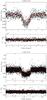 |
Fig. 9 Transits of CoRoT-25 (left) and CoRoT-26 (right). Top panels: light curve folded by the orbital period (black crosses) and the transit model computed from the most probable value of the different parameters (red line). Bottom panels: residuals after subtraction of this model; the red line is a smoothing over 30 points. |
6. Planetary system evolution models
In a first step, combined stellar and planetary evolution models of the CoRoT-25 and CoRoT-26 systems were calculated with SET and its new MCMC algorithm (Guillot & Havel 2011; Havel et al. 2011). Using a likelihood based on the stellar (respectively planetary) observables [Fe/H], Teff, ρ⋆, log g⋆ (respectively transit depth k, radial velocity K, log gp), and grids of models for the star and the planet, the MCMC explored the following parameter space: age, [Fe/H], M⋆, k, K, and dissipation in the planet (see below). The results are presented in terms of planetary radii as a function of age in Fig. 10. Solutions within 68.3%, 95.5%, and 99.7% confidence regions are shown with different colors.
Planetary evolution models were calculated in two cases: the standard case (which assumes that the thermal evolution of the planet is only a consequence of the loss of its primordial entropy through the irradiated planetary atmosphere; dashed lines in Fig. 10), and one in which a fraction of the incoming stellar light was assumed to be converted into kinetic energy and then dissipated at the center of the planet (plain lines in Fig. 10; see Guillot & Showman 2002; Guillot et al. 2006, for a discussion). The planets were assumed to be made of central ice and rock cores and solar-composition envelopes. The mass of the cores was varied between 0 (no core) and about 80% of Mp. Clearly, we do not know whether the heavy elements are present in the core or in the envelope, but this simple approach should generally provide a fair approximation of the global planetary composition (see Guillot et al. 2006; see however Baraffe et al. 2008).
These models were used in each step of the MCMC to infer the bulk composition (i.e., the mass of the core) of the planet using its age, mass, radius, and equilibrium temperature.
For CoRoT-25b (see Fig. 10, left panel), both the standard and dissipated-energy models provide solutions for the planetary radius that match the available constraints. However, this is not the case for CoRoT-26b, which is clearly oversized compared with standard evolution models (no dashed lines cross the 68.3% or 95.5% confidence regions in the right panel of Fig. 10) and hence requires an additional source of heat to explain its size, in line with what is inferred from a significant fraction of close-in transiting giant planets (e.g. Guillot et al. 2006; Laughlin et al. 2011; Batygin et al. 2011).
Considering the fact that dissipated-energy models are the most likely for both planets, we focused on theses solutions, and infered for CoRoT-25b a core mass of  , which translates into a heavy element mass fraction of
  . If standard models only were considered, CoRoT-25b would have a core mass of only ~10 M⊕.
On the other hand, CoRoT-26b has an estimated core mass of  , corresponding to a heavy-elements mass fraction of
  . This is in line with previous results for low-irradiated transiting giant planets (Miller & Fortney 2011).
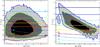 |
Fig. 10 Left: transit radius of CoRoT-25b as a function of age, as computed with SET. The 68.3%, 95.5%, and 99.7% confidence regions are denoted by three shades of gray. The curves represent the thermal evolution of a 0.27 MJ planet with an equilibrium temperature of 1330 K. Text labels indicate the amount of heavy elements in the planet (its core mass, in Earth masses). Solid lines represent planetary evolution models for which 0.25% of the incoming stellar flux is dissipated into the core of the planet, whereas dashed lines do not account for this dissipation (standard models). Right: the same for CoRoT-26b, for an 0.52 MJ planet with an equilibrium temperature of 1600 K. |
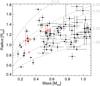 |
Fig. 11 Mass-radius diagram of transiting planets including CoRoT-25b and CoRoT-26b, Jupiter (J) and Saturn (S). The dashed lines correspond to 1.0, 0.5, 0.25, 0.20, and 0.10 Jupiter densities (data from exoplanets.org, Wright et al. 2011). |
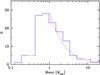 |
Fig. 12 Mass distribution of transiting giant planets. The dashed red curve corresponds to the relation N ~ M-1.14 per logarithmic mass unit. |
7. Conclusion
Figure 11 shows the location of these two new planets, CoRoT-25b and CoRoT-26b, in the mass-radius diagram of giant transiting planets. CoRoT-25b orbits an F9 main-sequence star with a period of 4.86 days. With a mass of 0.27 ± 0.04MJup and a radius of  , this planet is part of the Saturn-mass population (0.1−0.4 MJup ). The asymmetric errors in its radius are due to the high impact parameter,
  , which produces grazing transits.
CoRoT-26b orbits a slightly evolved G5 star, with an orbital period of 4.20 days. With a mass of 0.52 ± 0.05 MJup and a radius of  , CoRoT-26b is part of the low-mass hot-Jupiter population. The planet is inflated compared with standard evolution models and hence requires an additional source of energy to explain its radius. This is possibly given by dissipation of kinetic energy in the planet that had been received from the stellar insolation.
Figure 12 shows the mass distribution of transiting giant planets (Mp ≥ 0.1 MJup). Almost 50% of transiting giant planets have masses between 0.4 and 1.3 MJup. The sharp decrease of the distribution below 0.4 MJup, which corresponds to Saturn-like planets, is affected by the detection bias. In particular, its small radius population with radii below 0.8 RJup is dominantly detected by space missions. For stars with r′ < 15.5, the CoRoT detection capability is 66% for planetary radii between 0.35 and 0.45 RJup on G and K dwarfs, and periods shorter than 20 days (Bonomo et al. 2012). For larger planetary radii, the CoRoT detection capability is close to 100% (Bonomo, priv. comm.). According to results achieved with Kepler and CoRoT, only 15% of giant planets are part of the Saturn-like population (0.1−0.4 MJup ), which may indicate that this depletion is real. It is also worthwhile to note that the planet distribution follows an N ~ M-1.14 relation (per logarithm of the mass) for planets with masses greater than 1 MJup. This implies a distribution dN/dM close to M-2 as pointed out by Bouchy et al. (2009a), with a decrease toward massive giant planets more pronounced than claimed by Marcy et al. (2005, 2008) and slightly more pronounced than the synthetic planet mass distribution of Mordasini et al. (2009).
While the close-in giant population is well explored in the Jupiter-mass regime and higher, the Saturn-like population (0.1−0.4 MJup ) still remains too small to provide a robust basis for a significant statistical analysis. Almost 90% of transiting giant planets have indeed masses greater than 0.4 MJup. We note, however, that the few known members of this class have orbit-average equilibrium temperatures lower than 1400 K, except for HD149026b (Sato et al. 2005), one of the smallest Saturn-like planet with a highly dense core. The apparent lack of Saturns at higher temperatures (≳1400 K) may be an indication that such planets do not resist evaporation or/and that they lost most of their atmosphere (Mazeh et al. 2005; Lecavelier Des Etangs 2007; Ehrenreich & Désert 2011).
Acknowledgments
The team at IAC acknowledges support by grants AYA2010-20982-C02-02 and AYA2012-39346-C02-02 of the Spanish Ministerio de Economía y Competividad. Some of the data presented was acquired with the IAC80 telescope operated at Teide Observatory on the island of Tenerife by the Instituto de Astrofísica de Canarias. This research has made use of the Exoplanet Orbit Database and the Exoplanet Data Explorer at exoplanets.org. Part of this work was supported by a NASA Keck PI Data Award, administered by the NASA Exoplanet Science Institute. Some of the data presented herein were obtained at the W.M. Keck Observatory from telescope time allocated to the National Aeronautics and Space Administration through the agency’s scientific partnership with the California Institute of Technology and the University of California. The Observatory was made possible by the generous financial support of the W.M. Keck Foundation. The authors wish to recognize and acknowledge the very significant cultural role and reverence that the summit of Mauna Kea has always had within the indigenous Hawaiian community. We are most fortunate to have the opportunity to conduct observations from this mountain. This research was supported by an appointment to the NASA Postdoctoral Program at the Ames Research Center, administered by Oak Ridge Associated Universities through a contract with NASA.
References
- Alonso, R., Brown, T. M., Torres, G., et al. 2004, ApJ, 613, L153 [NASA ADS] [CrossRef] [Google Scholar]
- Alonso, R., Auvergne, M., Baglin, A., et al. 2008, A&A, 482, L21 [NASA ADS] [CrossRef] [EDP Sciences] [Google Scholar]
- Auvergne, M. 2006, in ESA SP 1306, eds. M. Fridlund, A. Baglin, J. Lochard, & L. Conroy, 283 [Google Scholar]
- Baglin, A., Auvergne, M., Barge, P., et al. 2009, in IAU Symp. 253, eds. F. Pont, D. Sasselov, & M. J. Holman, 71 [Google Scholar]
- Bakos, G. Á., Noyes, R. W., Kovács, G., et al. 2007, ApJ, 656, 552 [NASA ADS] [CrossRef] [Google Scholar]
- Baraffe, I., Chabrier, G., & Barman, T. 2008, A&A, 482, 315 [NASA ADS] [CrossRef] [EDP Sciences] [Google Scholar]
- Baranne, A., Queloz, D., Mayor, M., et al. 1996, A&AS, 119, 373 [NASA ADS] [CrossRef] [EDP Sciences] [Google Scholar]
- Barnes, S. A. 2007, ApJ, 669, 1167 [NASA ADS] [CrossRef] [Google Scholar]
- Batygin, K., Stevenson, D. J., & Bodenheimer, P. H. 2011, ApJ, 738, 1 [NASA ADS] [CrossRef] [Google Scholar]
- Bonomo, A. S., Santerne, A., Alonso, R., et al. 2010, A&A, 520, A65 [NASA ADS] [CrossRef] [EDP Sciences] [Google Scholar]
- Bonomo, A. S., Chabaud, P. Y., Deleuil, M., et al. 2012, A&A, 547, A110 [NASA ADS] [CrossRef] [EDP Sciences] [Google Scholar]
- Borucki, W. J., Koch, D., Basri, G., et al. 2010, Science, 327, 977 [NASA ADS] [CrossRef] [PubMed] [Google Scholar]
- Bouchy, F., Mayor, M., Lovis, C., et al. 2009a, A&A, 496, 527 [NASA ADS] [CrossRef] [EDP Sciences] [Google Scholar]
- Bouchy, F., Moutou, C., Queloz, D., & CoRoT Exoplanet Science Team 2009b, in IAU Symp. 253, eds. F. Pont, D. Sasselov, & M. J. Holman, 129 [Google Scholar]
- Cabrera, J., Bruntt, H., Ollivier, M., et al. 2010, A&A, 522, A110 [NASA ADS] [CrossRef] [EDP Sciences] [Google Scholar]
- Csizmadia, S., Pasternacki, T., Dreyer, C., et al. 2013, A&A, 549, A9 [NASA ADS] [CrossRef] [EDP Sciences] [Google Scholar]
- Cutri, R. M., Skrutskie, M. F., van Dyk, S., et al. 2003, 2MASS All Sky Catalog of point sources [Google Scholar]
- Deeg, H. J., Gillon, M., Shporer, A., et al. 2009, A&A, 506, 343 [NASA ADS] [CrossRef] [EDP Sciences] [Google Scholar]
- Deeg, H. J., Moutou, C., Erikson, A., et al. 2010, Nature, 464, 384 [NASA ADS] [CrossRef] [PubMed] [Google Scholar]
- Deleuil, M., Meunier, J. C., Moutou, C., et al. 2009, AJ, 138, 649 [NASA ADS] [CrossRef] [Google Scholar]
- Drummond, R., Vandenbussche, B., Aerts, C., De Oliveira Fialho, F., & Auvergne, M. 2006, PASP, 118, 874 [Google Scholar]
- Drummond, R., Lapeyrere, V., Auvergne, M., et al. 2008, A&A, 487, 1209 [NASA ADS] [CrossRef] [EDP Sciences] [MathSciNet] [Google Scholar]
- Ehrenreich, D., & Désert, J.-M. 2011, A&A, 529, A136 [NASA ADS] [CrossRef] [EDP Sciences] [Google Scholar]
- Endl, M., Kürster, M., & Els, S. 2000, A&A, 362, 585 [Google Scholar]
- Fridlund, M., Hébrard, G., Alonso, R., et al. 2010, A&A, 512, A14 [NASA ADS] [CrossRef] [EDP Sciences] [Google Scholar]
- Gandolfi, D., Alcalá, J. M., Leccia, S., et al. 2008, ApJ, 687, 1303 [NASA ADS] [CrossRef] [Google Scholar]
- Gandolfi, D., Hébrard, G., Alonso, R., et al. 2010, A&A, 524, A55 [NASA ADS] [CrossRef] [EDP Sciences] [Google Scholar]
- Gardes, B., Chabaud, P.-Y., & Guterman, P. 2011, in Proc. of the 2nd CoRoT Symp., 2, 119 [Google Scholar]
- Gillon, M., Demory, B.-O., Triaud, A. H. M. J., et al. 2009, A&A, 506, 359 [NASA ADS] [CrossRef] [EDP Sciences] [Google Scholar]
- Gregory, P. C. 2005, ApJ, 631, 1198 [NASA ADS] [CrossRef] [Google Scholar]
- Guillot, T., & Havel, M. 2011, A&A, 527, A20 [NASA ADS] [CrossRef] [EDP Sciences] [Google Scholar]
- Guillot, T., & Showman, A. P. 2002, A&A, 385, 156 [NASA ADS] [CrossRef] [EDP Sciences] [Google Scholar]
- Guillot, T., Santos, N. C., Pont, F., et al. 2006, A&A, 453, L21 [NASA ADS] [CrossRef] [EDP Sciences] [Google Scholar]
- Hauschildt, P. H., Allard, F., Ferguson, J., Baron, E., & Alexander, D. R. 1999, ApJ, 525, 871 [NASA ADS] [CrossRef] [Google Scholar]
- Havel, M., Guillot, T., Valencia, D., & Crida, A. 2011, A&A, 531, A3 [NASA ADS] [CrossRef] [EDP Sciences] [Google Scholar]
- Israelian, G., Delgado Mena, E., Santos, N. C., et al. 2009, Nature, 462, 189 [NASA ADS] [CrossRef] [PubMed] [Google Scholar]
- Laughlin, G., Crismani, M., & Adams, F. C. 2011, ApJ, 729, L7 [NASA ADS] [CrossRef] [Google Scholar]
- Lecavelier Des Etangs, A. 2007, A&A, 461, 1185 [NASA ADS] [CrossRef] [EDP Sciences] [Google Scholar]
- Mamajek, E. E., & Hillenbrand, L. A. 2008, ApJ, 687, 1264 [NASA ADS] [CrossRef] [Google Scholar]
- Mandel, K., & Agol, E. 2002, ApJ, 580, L171 [NASA ADS] [CrossRef] [Google Scholar]
- Marcy, G., Butler, R. P., Fischer, D., et al. 2005, Prog. Theor. Phys. Suppl., 158, 24 [NASA ADS] [CrossRef] [Google Scholar]
- Marcy, G. W., Butler, R. P., Vogt, S. S., et al. 2008, Phys. Scr. T, 130, 4001 [NASA ADS] [Google Scholar]
- Mazeh, T., Zucker, S., & Pont, F. 2005, MNRAS, 356, 955 [NASA ADS] [CrossRef] [Google Scholar]
- Miller, N., & Fortney, J. J. 2011, ApJ, 736, L29 [NASA ADS] [CrossRef] [Google Scholar]
- Mordasini, C., Alibert, Y., Benz, W., & Naef, D. 2009, A&A, 501, 1161 [NASA ADS] [CrossRef] [EDP Sciences] [Google Scholar]
- Pasternacki, T., Borde, P., & Csizmadia, S. 2011, in Proc. of the 2nd CoRoT Symp., 2, 117 [Google Scholar]
- Pepe, F., Mayor, M., Galland, F., et al. 2002, A&A, 388, 632 [NASA ADS] [CrossRef] [EDP Sciences] [Google Scholar]
- Pollacco, D. L., Skillen, I., Collier Cameron, A., et al. 2006, PASP, 118, 1407 [NASA ADS] [CrossRef] [Google Scholar]
- Pont, F., Hébrard, G., Irwin, J. M., et al. 2009, A&A, 502, 695 [NASA ADS] [CrossRef] [EDP Sciences] [Google Scholar]
- Rauer, H., Queloz, D., Csizmadia, S., et al. 2009, A&A, 506, 281 [NASA ADS] [CrossRef] [EDP Sciences] [Google Scholar]
- Sato, B., Fischer, D. A., Henry, G. W., et al. 2005, ApJ, 633, 465 [NASA ADS] [CrossRef] [Google Scholar]
- Surace, C., Alonso, R., Barge, P., et al. 2008, in SPIE Conf. Ser., 7019 [Google Scholar]
- Takeda, Y., Kawanomoto, S., Honda, S., Ando, H., & Sakurai, T. 2007, A&A, 468, 663 [NASA ADS] [CrossRef] [EDP Sciences] [Google Scholar]
- Wright, E. L., Eisenhardt, P. R. M., Mainzer, A. K., et al. 2010, AJ, 140, 1868 [NASA ADS] [CrossRef] [Google Scholar]
- Wright, J. T., Fakhouri, O., Marcy, G. W., et al. 2011, PASP, 123, 412 [NASA ADS] [CrossRef] [Google Scholar]
All Tables
All Figures
|
Fig. 1 CoRoT light curve from raw data of CoRoT-25 (top) and CoRoT-26 (bottom). The changes in sampling rates from 512 to 32 s appear as increases in the scatter. In gray dots, the 32 s integrations are binned to 512 s. The light curves show discontinuities due to the impact of high-energy particles and other instrumental effects. The transits can be seen as regular dips. |
| In the text | |
|
Fig. 2 POSS image of CoRoT-25 and CoRoT-26 (marked with a red cross in the center of the field) with the CoRoT mask superimposed (in blue solid line), and the contaminating stars (red crosses identified with a number, the contaminating R-magnitude its at the right of the image). |
| In the text | |
|
Fig. 3 Phase-folded radial velocities of CoRoT-25. The black circles and green squares correspond to HARPS and HIRES measurements. The red open circles correspond to the averages of the double (same night) measurements. |
| In the text | |
|
Fig. 4 HARPS bisector span versus radial velocities of CoRoT-25. The two red circles correspond to the averaged cross-correlation functions at the extreme phases of φ = 0.25 and 0.75. |
| In the text | |
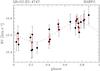 |
Fig. 5 Phase folded radial velocities of CoRoT-26. Symbols are similar to Fig. 3. |
| In the text | |
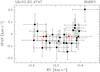 |
Fig. 6 HARPS bisector span versus radial velocities of CoRoT-26. Symbols are similar to Fig. 4. |
| In the text | |
|
Fig. 7 Optical and infrared photometric measurements (circles) and fitted spectral energy distributions (blue line) of CoRoT-25 (top) and CoRoT-26 (bottom). |
| In the text | |
|
Fig. 8 Two-parameter joint posterior distributions of all jump parameters for CoRoT-25 (left) and CoRoT-26 (right). The 68.3%, 95.5%, and 99.7% confidence regions are denoted by three different gray levels. PDFs are plotted at the bottom and the right of the panels. The dotted lines mark the maximum probability value of the PDF of each parameter. |
| In the text | |
|
Fig. 9 Transits of CoRoT-25 (left) and CoRoT-26 (right). Top panels: light curve folded by the orbital period (black crosses) and the transit model computed from the most probable value of the different parameters (red line). Bottom panels: residuals after subtraction of this model; the red line is a smoothing over 30 points. |
| In the text | |
|
Fig. 10 Left: transit radius of CoRoT-25b as a function of age, as computed with SET. The 68.3%, 95.5%, and 99.7% confidence regions are denoted by three shades of gray. The curves represent the thermal evolution of a 0.27 MJ planet with an equilibrium temperature of 1330 K. Text labels indicate the amount of heavy elements in the planet (its core mass, in Earth masses). Solid lines represent planetary evolution models for which 0.25% of the incoming stellar flux is dissipated into the core of the planet, whereas dashed lines do not account for this dissipation (standard models). Right: the same for CoRoT-26b, for an 0.52 MJ planet with an equilibrium temperature of 1600 K. |
| In the text | |
|
Fig. 11 Mass-radius diagram of transiting planets including CoRoT-25b and CoRoT-26b, Jupiter (J) and Saturn (S). The dashed lines correspond to 1.0, 0.5, 0.25, 0.20, and 0.10 Jupiter densities (data from exoplanets.org, Wright et al. 2011). |
| In the text | |
|
Fig. 12 Mass distribution of transiting giant planets. The dashed red curve corresponds to the relation N ~ M-1.14 per logarithmic mass unit. |
| In the text | |
Current usage metrics show cumulative count of Article Views (full-text article views including HTML views, PDF and ePub downloads, according to the available data) and Abstracts Views on Vision4Press platform.
Data correspond to usage on the plateform after 2015. The current usage metrics is available 48-96 hours after online publication and is updated daily on week days.
Initial download of the metrics may take a while.