| Issue |
A&A
Volume 555, July 2013
|
|
|---|---|---|
| Article Number | A53 | |
| Number of page(s) | 18 | |
| Section | Cosmology (including clusters of galaxies) | |
| DOI | https://doi.org/10.1051/0004-6361/201321256 | |
| Published online | 01 July 2013 | |
Experimental constraints on the uncoupled Galileon model from SNLS3 data and other cosmological probes
1
CEA,Centre de Saclay, Irfu/SPP,
91191
Gif-sur-Yvette,
France
e-mail:
This email address is being protected from spambots. You need JavaScript enabled to view it.
2
Center for Astrophysics and Space Astronomy, University of
Colorado, Boulder,
CO
80309-0389,
USA
3
LPNHE, Université Pierre et Marie Curie, Université Paris Diderot,
CNRS-IN2P3, 4 place
Jussieu, 75252
Paris Cedex 05,
France
4
Laboratoire de Physique Théorique d’Orsay, Bâtiment 210,
Université Paris-Sud 11, 91405
Orsay Cedex,
France
5
𝒢ℝεℂ𝒪, Institut d’Astrophysique de Paris, UMR 7095-CNRS, Université Pierre et Marie
Curie-Paris 6, 98bis boulevard
Arago, 75014
Paris,
France
Received:
7
February
2013
Accepted:
25
April
2013
Abstract
Aims. The Galileon model is a modified gravity theory that may provide an explanation for the accelerated expansion of the Universe. This model does not suffer from instabilities or ghost problems (normally associated with higher-order derivative theories), restores local General Relativity – thanks to the Vainshtein screening effect – and predicts late-time acceleration of the expansion.
Methods. We derive a new definition of the Galileon parameters that allows us to avoid having to choose initial conditions for the Galileon field. We tested this model against precise measurements of the cosmological distances and the rate of growth of cosmic structures.
Results. We observe a weak tension between the constraints set by growth data and those from distances. However, we find that the Galileon model remains consistent with current observations and is still competitive with the ΛCDM model, contrary to what was concluded in recent publications.
Key words: supernovae: general / cosmology: observations / dark energy
© ESO, 2013
1. Introduction
The discovery of the accelerated expansion of the Universe (Riess et al. 1998; Perlmutter et al. 1999) led cosmologists to introduce dark energy to explain our Universe. Adding a cosmological constant (Λ) to Einstein’s General Relativity is the simplest way to interpret observational data. However, even if adding a new fundamental constant is satisfactory, the value of Λ obtained from numerous measurements results in significant fine-tuning and coincidence problems. Thus, there is theoretical motivation to find alternative explanations, such as modified gravity models.
The Galileon model is just such a formulation. It was first proposed by Nicolis et al. (2009) as a general theory involving a scalar field, hereafter called π, and a second-order equation of motion invariant under a Galilean shift symmetry (∂μπ → ∂μπ + bμ, where bμ is a constant vector). This symmetry was first noticed in braneworld theories such as the DGP model of Dvali et al. (2000). The DGP model has the advantage of providing a self-accelerating solution to explain the expansion of the Universe, but it is plagued by ghost and instability problems. Galileon theories are a generalization of the DGP model that avoid these problems. The Galileon model was derived in a covariant formalism by Deffayet et al. (2009). It was also shown that this model forms a subclass of the general tensor-scalar theories involving only up to second-order derivatives originally found by Horndeski (1974).
In a four-dimension spacetime, only five Lagrangian terms are possible when forming an equation of motion for π invariant under the Galilean symmetry. Therefore, the Galileon Lagrangian has only five parameters. In the Galileon theory, as in the DGP theory, a screening mechanism called the Vainshtein effect (Vainshtein 1972) arises near massive objects due to non-linear derivative self-couplings of the π field. These ensure that the Galileon fifth force is screened near massive objects, and preserves General Relativity on local scales where it has been experimentally tested to high precision. However, this screening is only effective below a certain distance from massive objects (the Vainshtein radius) that depends on the mass of the object and on the values of the Galileon parameters (Burrage & Seery 2010). Experimental constraints on the Galileon parameters based on local tests of gravity have been proposed by Brax et al. (2011) and Babichev et al. (2011).
Recently, the Galileon model has been tested against observational cosmological data by Appleby & Linder (2012b), Okada et al. (2013), and Nesseris et al. (2010). These authors tend to reject the Galileon model because of tensions between growth-of-structure constraints and the other cosmological probes. The evolution of the Universe in the Galileon theory is based on differential equations involving the π field, which requires one to set initial conditions, and the above studies resorted to different methods for setting these initial conditions. In this work, we avoid this problem by introducing a new parametrization of the Galileon model that renders it independent of initial conditions. Combined with theoretical constraints derived in Appleby & Linder (2012a) and De Felice & Tsujikawa (2011), we compare our model with cosmological observables, and find that the Galileon model is not significantly disfavored by current observations.
We used the most recent measurements of Type Ia supernovae (SN Ia) luminosity distances, the cosmic microwave background (CMB), and baryon acoustic oscillations (BAO). The highest-quality SN Ia sample currently available is the SNLS3 sample described in Guy et al. (2010), Conley et al. (2011), and Sullivan et al. (2011). For the CMB, we used the observables from WMAP7 (Komatsu et al. 2011) and the set of BAO distances of the BOSS analysis (Sánchez et al. 2012). The growth of structures is an important probe for distinguishing modified gravity models from standard cosmological models such as ΛCDM, so it has to be used carefully. In this work, we used fσ8(z) measurements from several surveys, corrected for the Alcock-Paczynski effect.
Section 2 provides the Galileon equations used to compute the evolution of the Universe and the theoretical constraints imposed on the Galileon field. Section 3 describes the likelihood analysis, data samples, and the computing of cosmological observables. Section 4 gives the constraints on the Galileon model derived from data, and Sect. 5 discusses these results and their implications. We conclude in Sect. 6.
2. Cosmology with Galileons
2.1. Lagrangians
The Galileon model is based on the assumption that the scalar field equation of motion is
invariant under Galilean symmetries:
∂μπ → ∂μπ + bμ,
where bμ is a constant four vector. By
imposing this symmetry, Nicolis et al. (2009)
showed that there are only five possible Lagrangian terms Li
for the Galileon model action. The covariant formulation of the Galileon Lagrangian was
derived in Deffayet et al. (2009). In this paper we
start with this covariant action with the parametrization of Appleby & Linder (2012a): 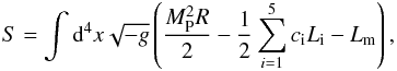 (1)with
Lm the standard-matter Lagrangian,
MP the Planck mass, R the Ricci scalar, and
g the determinant of the metric. The cis
are the arbitrary dimensionless parameters of the Galileon model that weight the different
terms. The Galileon Lagrangians have a covariant formulation derived in Deffayet et al. (2009):
(1)with
Lm the standard-matter Lagrangian,
MP the Planck mass, R the Ricci scalar, and
g the determinant of the metric. The cis
are the arbitrary dimensionless parameters of the Galileon model that weight the different
terms. The Galileon Lagrangians have a covariant formulation derived in Deffayet et al. (2009):
![Mathematical equation: \begin{eqnarray} L_1&=&M^3\pi,\quad L_2=(\nabla_\mu \pi)(\nabla^\mu \pi),\quad L_3=(\square \pi)(\nabla_\mu \pi)(\nabla^\mu \pi)/M^3 \notag \\ L_4&=&(\nabla_\mu \pi)(\nabla^\mu \pi)\left[ 2(\square \pi)^2 - 2 \pi_{;\mu\nu}\pi^{;\mu\nu} - R(\nabla_\mu \pi)(\nabla^\mu \pi)/2 \right]/M^6 \notag \\ L_5&=&(\nabla_\mu \pi)(\nabla^\mu \pi) \left[ (\square \pi)^3 - 3(\square \pi) \pi_{;\mu\nu}\pi^{;\mu\nu} +2\pi_{;\mu}\ ^{;\nu}\pi_{;\nu}\ ^{;\rho}\pi_{;\rho}\ ^{;\mu} \right.\notag \\ &&\left.-\,6 \pi_{;\mu}\pi^{;\mu\nu}\pi^{;\rho}G_{\nu\rho}\right]/M^9, \end{eqnarray}](/articles/aa/full_html/2013/07/aa21256-13/aa21256-13-eq15.png) (2)where
M is a mass parameter defined as
(2)where
M is a mass parameter defined as
 , where
H0 is the current value of the Hubble parameter. With this
definition the cis are dimensionless.
, where
H0 is the current value of the Hubble parameter. With this
definition the cis are dimensionless.
L2 is the usual kinetic term for a scalar field, while L3 to L5 are non-linear couplings of the Galileon field to itself, to the Ricci scalar R, and to the Einstein tensor Gμν, providing the necessary features for modifying gravity and mimicking dark energy. L1 is a tadpole term that acts as the usual cosmological constant, and may furthermore lead to vacuum instability because it is an unbounded potential term. Therefore, in the following we set c1 = 0.
Appleby & Linder (2012a) proposed
additional direct linear couplings to matter to add to the action: a linear coupling to
matter  and a derivative
coupling to matter
LG = cG∂μπ∂νπTμν/(MPM3),
which arises in some brane-world theories (see e.g. Trodden & Hinterbichler 2011), where
Tμν is the matter energy-momentum tensor.
These couplings may modify the physical origin of the accelerated expansion of the
Universe. Without coupling, the Universe is accelerated only because of the back-reaction
of the metric to the energy-momentum tensor of the scalar field, and the Galileon acts as
a dark energy component. If the Galileon is coupled directly to matter, instead, it can
give rise to accelerated expansion in the Jordan frame, while the Einstein-frame expansion
rate is not accelerating. In that case, the cosmic acceleration stems entirely from a
genuine modified gravity effect. In this work, we do not consider these optional
extensions to the theory, so the Einstein frame and Jordan frame coincide. For more
information about the Einstein and Jordan frames, see e.g. Faraoni et al. (1999).
and a derivative
coupling to matter
LG = cG∂μπ∂νπTμν/(MPM3),
which arises in some brane-world theories (see e.g. Trodden & Hinterbichler 2011), where
Tμν is the matter energy-momentum tensor.
These couplings may modify the physical origin of the accelerated expansion of the
Universe. Without coupling, the Universe is accelerated only because of the back-reaction
of the metric to the energy-momentum tensor of the scalar field, and the Galileon acts as
a dark energy component. If the Galileon is coupled directly to matter, instead, it can
give rise to accelerated expansion in the Jordan frame, while the Einstein-frame expansion
rate is not accelerating. In that case, the cosmic acceleration stems entirely from a
genuine modified gravity effect. In this work, we do not consider these optional
extensions to the theory, so the Einstein frame and Jordan frame coincide. For more
information about the Einstein and Jordan frames, see e.g. Faraoni et al. (1999).
Action 1 leads to three differential equations: two Einstein equations ((00) temporal component and (ij) spatial component) coming from the variation of the action with respect to the metric gμν, and the scalar field equation of motion from the variation of the action with respect to the π field. The equations are given explicitly in Appendix B of Appleby & Linder (2012a). With these three differential equations the evolution of the Universe and the dynamics of the field can be computed.
To solve the cosmological equations, we chose the Friedmann-Lemaître-Robertson-Walker (FLRW) metric. With no direct couplings, the functions to compute are the Hubble parameter H = ȧ/a (with a the cosmic scale factor), and x = π′/MP, with a prime denoting d/dlna (see Appleby & Linder 2012a and Sect. 2.3).
2.2. Initial conditions
To compute the solutions of the above equations, we need to set one initial condition for
x. We arbitrarily chose to define this initial condition at
z = 0, which we denote
x0 = x(z = 0).
Unfortunately, we have no prior information about the value of the Galileon field or its
derivative at any epoch. Fortunately, x0 can be absorbed by
redefining the cis as follows:
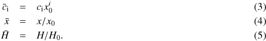 This
redefinition allows us to avoid treating x0 as an extra free
parameter of the model1. Doing so, the
This
redefinition allows us to avoid treating x0 as an extra free
parameter of the model1. Doing so, the
 s
remain dimensionless, and the initial conditions are simple:
s
remain dimensionless, and the initial conditions are simple:
 (6)Note that the (00)
Einstein equation could also be used as a constraint equation to fix
x0 (see Appendix A) given a set of cosmological parameters
cis,
(6)Note that the (00)
Einstein equation could also be used as a constraint equation to fix
x0 (see Appendix A) given a set of cosmological parameters
cis,  and
and
 . If we were
to adapt this, we would observe a degeneracy between the parameters: the same cosmological
evolution can be obtained with small cis and a high
x0, or with high cis and a small
x0. In other words, different sets of parameters
{ci,x0} produce
the same cosmology, i.e., the same
ρπ(z), which is
undesirable. Our parametrization avoids this problem by absorbing the degeneracy between
the cis and x0 into our
s.
. If we were
to adapt this, we would observe a degeneracy between the parameters: the same cosmological
evolution can be obtained with small cis and a high
x0, or with high cis and a small
x0. In other words, different sets of parameters
{ci,x0} produce
the same cosmology, i.e., the same
ρπ(z), which is
undesirable. Our parametrization avoids this problem by absorbing the degeneracy between
the cis and x0 into our
s.
2.3. Cosmological equations
To compute cosmological evolution in the Galileon model, we assume for simplicity that
the Universe is spatially flat, in agreement with current observations. We used the
Friedmann-Lemaître-Robertson-Walker (FLRW) metric in a flat space:
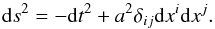 (7)When writing the
cosmological equations, we can mix the (ij) Einstein equation and the π
equation of motion to obtain the following system of differential equations for
(7)When writing the
cosmological equations, we can mix the (ij) Einstein equation and the π
equation of motion to obtain the following system of differential equations for
 and
and  :
:
 with
with
 as
derived in the formalism of Appleby & Linder
(2012a), but using our normalization for the cis. We
obtain the same equations except that the cis are changed into
s,
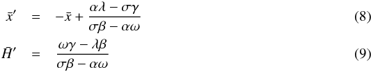
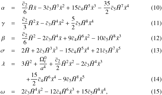
and that we have a different treatment for the initial conditions. Equations (8) and (9) depend only on the s
and . The
radiation energy density in Eq. (14) is
computed from the usual formula
as
derived in the formalism of Appleby & Linder
(2012a), but using our normalization for the cis. We
obtain the same equations except that the cis are changed into
s,
and that we have a different treatment for the initial conditions. Equations (8) and (9) depend only on the s
and . The
radiation energy density in Eq. (14) is
computed from the usual formula 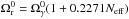 with
Neff = 3.04 the standard effective number of neutrino
species (Mangano et al. 2002). The photon energy
density at the current epoch is given by
with
Neff = 3.04 the standard effective number of neutrino
species (Mangano et al. 2002). The photon energy
density at the current epoch is given by 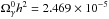 (where, as usual,
h = H0/(100
km s Mpc-1) for TCMB = 2.725 K.
(where, as usual,
h = H0/(100
km s Mpc-1) for TCMB = 2.725 K.
2.4. Perturbation equations
To test the Galileon model predictions for the growth of structures, we also need the
equations describing density perturbations. We followed the approach of Appleby & Linder (2012a) for the scalar
perturbation. Appleby & Linder (2012a)
performed their computation in the frame of the Newtonian gauge, for scalar modes in the
subhorizon limit, with the following perturbed metric:
 (16)In this context, the
perturbed equations of the (00) Einstein equation, the (ij) Einstein equation, the
π equation of motion, and the equation of state of matter are in the
quasi-static approximation
(16)In this context, the
perturbed equations of the (00) Einstein equation, the (ij) Einstein equation, the
π equation of motion, and the equation of state of matter are in the
quasi-static approximation 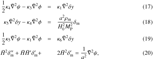 where
δy = δπ/MP
is the perturbed Galileon,
where
δy = δπ/MP
is the perturbed Galileon,  ,
ρm is the matter density, and
δm = δρm/ρm
is the contrast matter density. κis are the same as in Appleby & Linder (2012a), but rewritten
following our parametrization:
,
ρm is the matter density, and
δm = δρm/ρm
is the contrast matter density. κis are the same as in Appleby & Linder (2012a), but rewritten
following our parametrization: 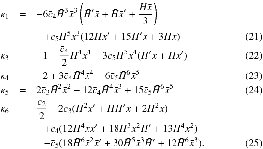 With
Eqs. (17) to (20), we can obtain a Poisson equation for ψ, with an
effective gravitational coupling
With
Eqs. (17) to (20), we can obtain a Poisson equation for ψ, with an
effective gravitational coupling  that
varies with time and depends on the Galileon model parameters
s:
that
varies with time and depends on the Galileon model parameters
s:
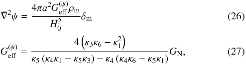 with
GN Newton’s gravitational constant. These equations can be
used to compute the growth of matter perturbations in the frame of the Galileon model (see
Sect. 3.2.4). Tensorial perturbations modes also
exist, and are studied in Sect. 2.5.4.
with
GN Newton’s gravitational constant. These equations can be
used to compute the growth of matter perturbations in the frame of the Galileon model (see
Sect. 3.2.4). Tensorial perturbations modes also
exist, and are studied in Sect. 2.5.4.
2.5. Theoretical constraints
With so many parameters, it is necessary to restrict the parameter space theoretically before comparing the model to data. The theoretical constraints arise from multiple considerations: the (00) Einstein equation, requiring positive energy densities, and avoiding instabilities in scalar and tensorial perturbations.
2.5.1. The (00) Einstein equation and 
Because we used only the (ij) Einstein equation and the π equation of
motion to compute the dynamics of the Universe (Eqs. (8) and (9)), we are
able to use the (00) Einstein equation as a constraint on the model parameters:
 (28)
More precisely, we used
this constraint both at z = 0 to fix one of our parameters and, at
other redshifts, to check the reliability of our numerical computations (see Sect. 3.1). The parameter we chose to fix at
z = 0 is
(28)
More precisely, we used
this constraint both at z = 0 to fix one of our parameters and, at
other redshifts, to check the reliability of our numerical computations (see Sect. 3.1). The parameter we chose to fix at
z = 0 is 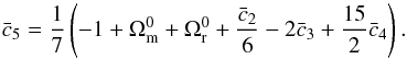 (29)We chose to fix
 based on the other parameters because allowing it to float introduces significant
numerical difficulties when solving Eqs. (8) and (9), since it represents
the weight of the most non-linear term in these equations. As
is fixed
given h, our parameter space has been reduced to
based on the other parameters because allowing it to float introduces significant
numerical difficulties when solving Eqs. (8) and (9), since it represents
the weight of the most non-linear term in these equations. As
is fixed
given h, our parameter space has been reduced to
 and
and
 .
.
2.5.2. Positive energy density
We require that the energy density of the Galileon field be positive from
z = 0 to z = 107 (see Sect. 3.2.2 and Appendix B). At every redshift in this
range, this constraint amounts to 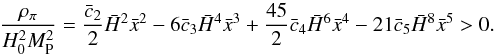 (30)This constraint
is not really necessary for generic scalar field models. But as we will see in the
following, it has no impact on our analysis because the other theoretical conditions
described below are stronger.
(30)This constraint
is not really necessary for generic scalar field models. But as we will see in the
following, it has no impact on our analysis because the other theoretical conditions
described below are stronger.
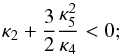
2.5.3. Scalar perturbations
As suggested by Appleby & Linder (2012a), outside the quasi-static approximation the propagation equation for δy leads to two conditions, which we again checked from z = 0 to z = 107 to ensure the viability of the linearly perturbed model:
-
1.
a no-ghost condition, which requires a positive energy for theperturbation
 (31)
(31) -
2.
a Laplace stability condition for the propagation speed of the perturbed field
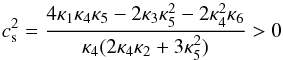 (32)
(32)
 (33)
(33)
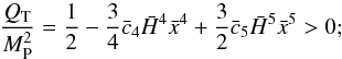
2.5.4. Tensorial perturbations
We also addrd two conditions derived by De Felice
& Tsujikawa (2011) for the propagation of tensor perturbations.
Considering a traceless and divergence-free perturbation
δgij = a2hij,
these authors obtained identical perturbed actions at second order for each of the two
polarisation modes h⊕ and h⊗.
For
h⊕![Mathematical equation: \begin{equation} \delta S_{\rm T}^{(2)}=\frac{1}{2}\int {\rm d}td^3xa^3Q_{\rm T}\left[\dot h^2_\oplus - \frac{c_{\rm T}^2}{a^2}(\nabla h_\oplus)^2 \right] \end{equation}](/articles/aa/full_html/2013/07/aa21256-13/aa21256-13-eq83.png) (34)with
QT and cT as defined below.
From that equation, we extracted two conditions in our parametrization that have to be
satisfied (again from z = 0 to
z = 107):
(34)with
QT and cT as defined below.
From that equation, we extracted two conditions in our parametrization that have to be
satisfied (again from z = 0 to
z = 107):
-
1.
a no-ghost condition:
 (35)
(35) -
2.
a Laplace stability condition:
 (36)
(36)
s,
as pointed out in e.g. Barreia et al. (2012). The
above theoretical constraints and our new parametrization allowed us to break
degeneracies between the
parameters that would make it difficult to converge to a unique best-fit with current
cosmological observations. As an example, the tensorial theoretical conditions lead to a
significant reduction of the parameter space (see dark dotted regions in Fig. 2), so that closed probability contours are obtained.
3. Likelihood analysis method and observables
In the following, we define a scenario to be a specific realisation of the cosmological
equations for a given set of parameters  .
.
To perform the likelihood analysis, the method used in Conley et al. (2011) for the analysis of SNLS data2 was adapted to the Galileon model. For each cosmological probe, a likelihood
surface ℒ was derived by computing the χ2 for each visited
scenario:  . The way
h is treated is described in Sect. 3.2.2. Then we report the mean value of the marginalized parameters as the fit
values of and the
s.
. The way
h is treated is described in Sect. 3.2.2. Then we report the mean value of the marginalized parameters as the fit
values of and the
s.
3.1. Numerical computation method
To compute numerical solutions to Eqs. (8)
and (9), we used a fourth-order Runge-Kutta
method to compute  and
and  iteratively starting from the current epoch, where the initial conditions for
and
are specified (see 2.2), and propagating backwards in
time to higher z. We used a sufficiently small step size in
z to avoid numerical divergences. This is challenging because of the
significant non-linearities in our equations. To determine the step size, we therefore
required that Eq. (28), normalized by
iteratively starting from the current epoch, where the initial conditions for
and
are specified (see 2.2), and propagating backwards in
time to higher z. We used a sufficiently small step size in
z to avoid numerical divergences. This is challenging because of the
significant non-linearities in our equations. To determine the step size, we therefore
required that Eq. (28), normalized by
 ,
be satisfied at better than 10-5 for each step.
,
be satisfied at better than 10-5 for each step.
At each step of the computation, we also checked that all previously discussed theoretical conditions were satisfied (Eqs. (30)–(32), (35), and (36)). Cosmological scenarios that fail any of these conditions were rejected and their likelihood set to zero. The result of these requirements is shown e.g. in Fig. 2 as dark dotted regions. Equation (30) concerns a negligible number of Galileon scenarios, but the four other constraints lead to a significant reduction of the parameter space.
3.2. Data
Here we describe the cosmological observations we used in our analysis. Special care was taken to choose data that do not depend on additional cosmological assumptions.
3.2.1. Type Ia supernovae
The SN Ia data sample used in this work is the SNLS3 sample described in Conley et al. (2011). It consists of 472 well-measured supernovae from the SNLS, SDSS, HST, and a variety of low-z surveys.
A Type Ia supernova with intrinsic stretch s and color
 has a rest-frame B-band apparent magnitude
mB that can be modeled as follows:
has a rest-frame B-band apparent magnitude
mB that can be modeled as follows:
 (37)where
 is the Hubble-constant free luminosity distance, which in a flat Universe is given by
 (38)zhel
and zCMB are the SN Ia redshift in the heliocentric and CMB
rest frames, respectively, “cosmo” represents the cosmological parameters of the model.
α and β are parameters describing the light-curve
width-luminosity and color-luminosity relationships for SNe Ia. ℳℬ is defined
as
ℳℬ = MB + 5log 10c/H0 + 25,
where MB is the rest-frame absolute
magnitude of a fiducial (
(38)zhel
and zCMB are the SN Ia redshift in the heliocentric and CMB
rest frames, respectively, “cosmo” represents the cosmological parameters of the model.
α and β are parameters describing the light-curve
width-luminosity and color-luminosity relationships for SNe Ia. ℳℬ is defined
as
ℳℬ = MB + 5log 10c/H0 + 25,
where MB is the rest-frame absolute
magnitude of a fiducial ( )
SN Ia in the B-band, and
c/H0 is expressed in
Mpc. α,β and ℳℬ are nuisance parameters that are fit
simultaneously with the cosmological parameters. As in Conley et al. (2011) and Sullivan et al.
(2011), we allowed for different ℳℬ in galaxies with the host galaxy
stellar mass below and above 1010 M⊙ to account
for relations between SN Ia brightness and host properties that are not corrected for
via the standard s and
relations. When computing Type Ia supernova distance luminosities in Sect. 4, we neglect the radiation component in
)
SN Ia in the B-band, and
c/H0 is expressed in
Mpc. α,β and ℳℬ are nuisance parameters that are fit
simultaneously with the cosmological parameters. As in Conley et al. (2011) and Sullivan et al.
(2011), we allowed for different ℳℬ in galaxies with the host galaxy
stellar mass below and above 1010 M⊙ to account
for relations between SN Ia brightness and host properties that are not corrected for
via the standard s and
relations. When computing Type Ia supernova distance luminosities in Sect. 4, we neglect the radiation component in
 ,
since all measurements are restricted to redshifts below 1.4 where the effects of
radiation density are negligible.
,
since all measurements are restricted to redshifts below 1.4 where the effects of
radiation density are negligible.
Systematic uncertainties must be treated carefully when using SN Ia data, because they depend on α and β and due to covariances between different supernovae. We followed the treatment of Conley et al. (2011) and Sullivan et al. (2011).
3.2.2. Cosmological microwave background
The CMB is a powerful probe to constrain the expansion history of the Universe because it gives high-redshift cosmological observables. The power spectrum provides much information on the content of the Universe and the relations between the different fluids, as long as we are able to model the thermodynamics of these fluids before recombination. The Galileon model does not modify the standard baryon-photon flux physics as long as the Galileon field does not couple directly to matter, as is assumed in this work. Thus, the usual formulae and predictions used in the standard analysis of the CMB power spectrum remain valid.
The positions of the acoustic peaks can be quantified by three observables:
{la,R,z∗}
(see e.g. Komatsu et al. 2011 and Komatsu et al. 2009), where
la is the acoustic scale related to the comoving sound
speed horizon, R is the shift parameter related to the distance between
us and the last scattering surface, and z∗ is the redshift
of the last scattering surface. These quantities are derived from the angular diameter
distance, which in a flat space is given by
 (39)and from the
comoving sound speed horizon:
(39)and from the
comoving sound speed horizon:  (40)
(40) is the usual normalized sound speed in the baryon-photon fluid before recombination:
 (41)where
 is the
baryon energy density parameter today.
is the
baryon energy density parameter today.
With the above definitions, the acoustic scale la is given
by  (42)and the shift parameter
R by
(42)and the shift parameter
R by  (43)z∗
is given by the fitting formula of Hu & Sugiyama
(1996):
(43)z∗
is given by the fitting formula of Hu & Sugiyama
(1996): ![Mathematical equation: \begin{eqnarray} \label{eq:zstar} &&z_*=1048\left[1+0.00124(\Omega_{\rm b}^0h^2)^{-0.738}\right] \left[1+g_1(\Omega_{\rm m}^0h^2)^{g_2}\right] \\ &&g_1=\frac{0.0783(\Omega_{\rm b}^0h^2)^{-0.238}}{1+39.5(\Omega_{\rm b}^0h^2)^{0.763}}\\ &&g_2=\frac{0.560}{1+21.1(\Omega_{\rm b}^0h^2)^{1.81}}\cdot \end{eqnarray}](/articles/aa/full_html/2013/07/aa21256-13/aa21256-13-eq126.png) According
to Hu & Sugiyama (1996), formula (44) is valid for a wide range of
According
to Hu & Sugiyama (1996), formula (44) is valid for a wide range of
 and
and
 .
.
BAO measurements.
To compare these observables with the seven-year WMAP data (WMAP7), we followed the
numerical recipe given in Komatsu et al. (2009).
The key point of this recipe is that for each cosmological scenario,
 must be minimized
over h and , which appear in
Eq. (44) and in the computation of
through (see Eq.
(14)).
must be minimized
over h and , which appear in
Eq. (44) and in the computation of
through (see Eq.
(14)).
An important feature to note is that we have to solve Eqs. (8) and (9) from a = 1 to a = 0 to compute the CMB observables. Numerically, however, we cannot reach a = 0 (z = ∞) because of numerical divergences. To avoid them, we carried out these computations up to a = 10-7 and then linearly extrapolated the value of the integral to a = 0 (for more details on the reliability of this approximation see Appendix B). Thus, the theoretical constraints of 2.5 were checked from a = 1 to a = 10-7.
Finally, because CMB observables depend explicitly on H0, we imposed a Gaussian prior on its value, h = 0.737 ± 0.024 as measured by Riess et al. (2011) from low-redshift SNe Ia and Cepheid variables.
The WMAP7 recommended best-fit values of the CMB observables are
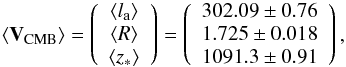 (47)with the corresponding
inverse covariance matrix:
(47)with the corresponding
inverse covariance matrix: 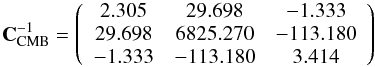 (48)from
Komatsu et al. (2011). As pointed out by Nesseris et al. (2010), the uncoupled Galileon model
fulfils the assumptions required in Komatsu et al.
(2009) to use these distance priors, namely a FLRW Universe with the standard
number of neutrinos and a dark energy background with negligible interactions with the
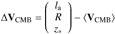
primordial Universe. Once the observables
{la,R,z∗}
were computed in a cosmological scenario, we built the difference vector:
(48)from
Komatsu et al. (2011). As pointed out by Nesseris et al. (2010), the uncoupled Galileon model
fulfils the assumptions required in Komatsu et al.
(2009) to use these distance priors, namely a FLRW Universe with the standard
number of neutrinos and a dark energy background with negligible interactions with the
primordial Universe. Once the observables
{la,R,z∗}
were computed in a cosmological scenario, we built the difference vector:
 (49)and computed
the CMB contribution to the total χ2 :
(49)and computed
the CMB contribution to the total χ2 :
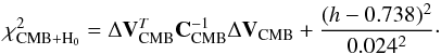 (50)
(50)
3.2.3. Baryonic acoustic oscillations
BAO distances provide information on the imprint of the comoving sound horizon after
recombination on the distribution of galaxies. The BAO observable is defined as
ys(z) = rs(zd)/DV(z),
where rs is the comoving sound horizon at the baryon drag
epoch redshift zd, and
DV(z) is the effective
distance (Eisenstein et al. 2005) given by
![Mathematical equation: \begin{equation} D_V(z)=\left[(1+z)^2D_{\rm A}^2(z)\frac{cz}{H(z)}\right]^{1/3}\cdot \end{equation}](/articles/aa/full_html/2013/07/aa21256-13/aa21256-13-eq148.png) (51)zd
is computed using the Eisenstein & Hu
(1998) fitting formula:
(51)zd
is computed using the Eisenstein & Hu
(1998) fitting formula: ![Mathematical equation: \begin{eqnarray} z_{\rm d}&=&\frac{1291(\Omega_{\rm m}^0h^2)^{0.251}}{1+0.659(\Omega_{\rm m}^0h^2)^{0.828}} \left[1+b_1(\Omega_{\rm b}^0h^2)^{b_2}\right] \\ b_1 &=& 0.313(\Omega_{\rm m}^0h^2)^{-0.419} \left[1+0.607(\Omega_{\rm m}^0h^2)^{0.674}\right] \\ b_2 &=& 0.238(\Omega_{\rm m}^0h^2)^{0.223} . \end{eqnarray}](/articles/aa/full_html/2013/07/aa21256-13/aa21256-13-eq149.png) This
formula remains valid for a Galileon field not coupled to matter.
This
formula remains valid for a Galileon field not coupled to matter.
Therefore BAO distances depend on h and
as the
CMB observables so we followed the same recipe as previously mentioned to compute them,
including the H0 prior from Riess et al. (2011). We also made the same approximation as for the CMB to
compute rs. The minimization over h and
was performed
independently for CMB and BAO when their individual constraints are derived and
simultaneously when combined constraints were computed.
We used the dataset of distances derived from galaxy surveys as published in the SDSS-III BOSS cosmological analysis (Anderson et al. 2012 and Sánchez et al. 2012) to avoid redshift overlaps in the measurements (see Table 1).
For a cosmological constraint derived from BAO distances alone, the BAO contribution to
the total χ2 is given by 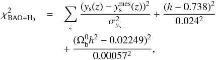 (55)where
we added a Gaussian prior on when dealing with
this probe alone.
(55)where
we added a Gaussian prior on when dealing with
this probe alone.
When BAO and CMB probes were combined, we computed their contributions to the
χ2 simultaneously to avoid over-counting the Hubble
constant prior. Therefore, the combined contribution is
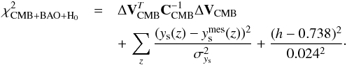 (56)
(56)
Growth data.
Cosmological constraints on the Galileon model from the SNLS3 sample.
3.2.4. Growth rate of structures
The cosmological growth of structures is a critical test of the Galileon model, as noted by many authors (see Linder 2005 for example). It is a very discriminant constraint for distinguishing dark energy and modified gravity models. Many models can mimic ΛCDM behavior for the expansion history of the Universe, but all modify gravity and structure formation in a different manner.
In linear perturbation theory, the growth of a matter perturbation
δm = δρm/ρm
is governed by the equation 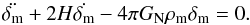 (57)But as argued in
Linder (2005) and as used in Komatsu et al. (2009), it is better to study the
growth evolution with the function
g(a) ≡ D(a)/a ≡ δm(a)/(aδm(1)).
In the Galileon case, the Newton constant is replaced by
(57)But as argued in
Linder (2005) and as used in Komatsu et al. (2009), it is better to study the
growth evolution with the function
g(a) ≡ D(a)/a ≡ δm(a)/(aδm(1)).
In the Galileon case, the Newton constant is replaced by
 as given in Eq. (27). The
g(a) is obtained by solving the following
second-order differential equation
as given in Eq. (27). The
g(a) is obtained by solving the following
second-order differential equation 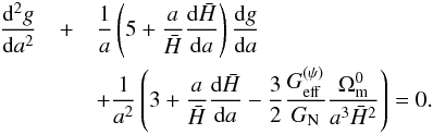 (58)A
natural choice for the initial conditions is
g(ainitial) = 1 and
dg/da|ainitial = 0
(Komatsu et al. 2009), where
ainitial is
0.001 ≈ 1/(1 + z∗). We checked that our
results do not depend on this choice as long as ainitial is
taken between 10-2 and 10-5.
(58)A
natural choice for the initial conditions is
g(ainitial) = 1 and
dg/da|ainitial = 0
(Komatsu et al. 2009), where
ainitial is
0.001 ≈ 1/(1 + z∗). We checked that our
results do not depend on this choice as long as ainitial is
taken between 10-2 and 10-5.
Measurements of the rate of growth of cosmic structures from redshift space distortions
can be expressed in terms of
f(a) = dlnD(a)/dlna
or fσ8(a), where
σ8 is the normalization of the matter power spectrum.
fσ8(a) is known to be
less sensitive to the overall normalization of the power spectrum model used to derive
the measurements (Song & Percival 2009).
Accordingly this is the observable we chose in this work. To predict
fσ8(a) in our analysis,
we solved Eq. (58) to obtain
g(a), from which we deduced
f(a) and D(a), and
we computed σ8(a) in the following way
(Samushia et al. 2012a): 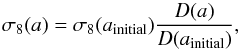 (59)where
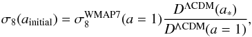 (60)and
 is the present value of the CMB power spectrum normalization published by Komatsu et al. (2011) in the framework of the ΛCDM
model. Equation (60) states that the
normalization of the CMB power spectrum at decoupling is the same in the ΛCDM and
Galileon models, which is consistent with our assumption that the CMB physics is not
modified by the Galileon presence. This equation holds if
D(a) has no scale dependence, which is the case in
both models in the linear regime. Equation (59) takes into account the different growth histories since recombination in
the two models.
is the present value of the CMB power spectrum normalization published by Komatsu et al. (2011) in the framework of the ΛCDM
model. Equation (60) states that the
normalization of the CMB power spectrum at decoupling is the same in the ΛCDM and
Galileon models, which is consistent with our assumption that the CMB physics is not
modified by the Galileon presence. This equation holds if
D(a) has no scale dependence, which is the case in
both models in the linear regime. Equation (59) takes into account the different growth histories since recombination in
the two models.
However, stand-alone fσ8(a) measurements extracted from observed matter power spectra usually use a fiducial cosmology, which assumes General Relativity. This hypothesis is no longer necessary when taking into account the Alcock-Paczynski effect (Alcock & Paczynski 1979) in the power spectrum analysis. This results in joint measurements of fσ8(a) and the Alcock-Paczynski parameter F(a) ≡ c-1DA(a)H(a)/a, which are to be preferred when constraining modified gravity models (see e.g. Beutler et al. 2012 and Samushia et al. 2012b). Note that Eqs. (8) and (9) are all we need to predict F(a) in the Galileon model.
The measurements of
fσ8(z) and
F(z) used in this work are summarized in Table 2. To compare these with our model, we first solved
Eqs. (8) and (9) from a = 1 to
ainitial to obtain values of
 ,
F(a) and
,
F(a) and  , and then
solved Eq. (58) from
ainitial to a = 1, which provides us with
fσ8(z) predictions.
, and then
solved Eq. (58) from
ainitial to a = 1, which provides us with
fσ8(z) predictions.
Galileon model best-fit values from different data samples.
Because F(z) and
fσ8(z) measurements are
correlated, a covariance matrix CGoS was built using data
presented in Table 2. Moreover, our
fσ8 prediction relies on the WMAP7
measurement of σ8(a = 1) (Eq. (60)), so the WMAP7 experimental uncertainty
is also propagated to the diagonal and off-diagonal terms of
CGoS. Then a vector VGoS containing
all predictions at each zi was built
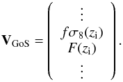 (61)The contribution of the
growth rate of structures to the total χ2 is then
(61)The contribution of the
growth rate of structures to the total χ2 is then
 (62)with
ΔVGoS = VGoS − ⟨ VGoS ⟩,
where ⟨ VGoS ⟩ contains the measurements of Table 2.
(62)with
ΔVGoS = VGoS − ⟨ VGoS ⟩,
where ⟨ VGoS ⟩ contains the measurements of Table 2.
Note that Eq. (14) requires a value for
, and
hence in principle this equation should be simultaneously solved with the BAO and CMB
constraints using the same prior on H0. However, we found
that this has essentially no effect on our χ2. Therefore, we
set here h to the value derived from the H0
measurements of Riess et al. (2011) to accelerate
the computation.
4. Results
In the following we present the results of the experimental constraints on the Galileon model derived from the cosmological probes.
4.1. SN constraints
Results from SN Ia data are presented in Fig. 2 and Table 3.
4.1.1. SN results
Despite the large number of free parameters in the model, we obtained closed
probability contours in any two-dimensional projection of the parameter space. We
observed strong correlations between the s,
especially between  and
and  .
.
We note that the best-fit value for  is
compatible with the current constraints obtained in the ΛCDM or FWCDM models. The
s
are found to be globally of the order of ≈− 1. From the best-fit values of the
parameters, we derived the value of
using Eq. (29) and find
is
compatible with the current constraints obtained in the ΛCDM or FWCDM models. The
s
are found to be globally of the order of ≈− 1. From the best-fit values of the
parameters, we derived the value of
using Eq. (29) and find
 ,
including systematic uncertainties.
,
including systematic uncertainties.
In the following we discuss the impact of fixing the nuisance parameters α and β and the effect of systematics on the best-fit values.
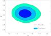 |
Fig. 1 Confidence contours for the SN nuisance parameters α and β when marginalizing over all other parameters of the model. Dashed red contours represent 68.3%, 95.4%, and 99.7% probability contours for the ΛCDM model. Filled blue contours are for the Galileon model. Note that they are nearly identical, the Galileon one is just 2.8% wider, which is likely due to larger steps in α and β. See Table 3 for numerical values. |
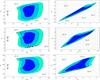 |
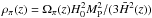
Fig. 2 Experimental constraints on the Galileon model from SNLS3 data alone. To
represent the four-dimensional likelihood |

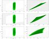 |
Fig. 3 Experimental constraints on the Galileon model from WMAP7+BAO+H0 data. To
represent the four-dimensional likelihood |
4.1.2. Impact of nuisance parameters
When marginalizing over the cosmological parameters, the best-fit values of the SN
nuisance parameters α, β,
 , and
, and
 in the
Galileon context are identical to those published for the ΛCDM model, as shown in Fig.
1 and Table 3. This is a truly important point to note. It means that the modeling of the
SN Ia physics contained in these nuisance parameters is adequate for these two
cosmological models despite their differences.
in the
Galileon context are identical to those published for the ΛCDM model, as shown in Fig.
1 and Table 3. This is a truly important point to note. It means that the modeling of the
SN Ia physics contained in these nuisance parameters is adequate for these two
cosmological models despite their differences.
In principle, the correct method to use when analyzing SN Ia data is to scan and marginalize over the nuisance parameters. However, once the best-fit values of α and β are known, keeping them fixed to their best-fit values in any study using the same SN sample has a negligible impact on our results (see Table 3). In the Galileon case, the contour areas decrease by only 0.7% and have the same shape as in Fig. 2. For future studies with the SNLS3 sample in the ΛCDM or Galileon models, our analysis therefore demonstrates that it is reasonable to keep the nuisance parameters fixed to the values published the SNLS papers.
4.1.3. Impact of systematic uncertainties
From the results in Table 3, we note that the identified systematic uncertainties shift the best-fit values of the Galileon parameters by less than their statistical uncertainties. With systematics included, the area of the inner contours increases by about 53%. This is less than what is observed in fits to the ΛCDM or FWCDM models (103% and 80% respectively, see Conley et al. 2011).
4.2. Combined CMB, BAO, and H0 constraints
The results using CMB, BAO, and H0 data are presented in Fig. 3 and Table 4.
The combined WMAP7+BAO+H0 data provide a very powerful constraint on
, but no
tighter constraints on the
than SNe Ia alone.  is, as for the SNLS3 sample, close to the current best estimates for this parameter in the
standard cosmologies, but this time with very sharp error bars competitive with the most
recent studies on other cosmological models. However, the
best-fit values are similar to those predicted with the SNLS3 sample.
is, as for the SNLS3 sample, close to the current best estimates for this parameter in the
standard cosmologies, but this time with very sharp error bars competitive with the most
recent studies on other cosmological models. However, the
best-fit values are similar to those predicted with the SNLS3 sample.
To use the WMAP7+BAO+H0 data, h and
have to be minimized
for each explored Galileon scenario. Minimized values of these parameters are collected in
the histograms of Fig. 4 for the subset of the
scenarios that fulfilled the theoretical constraints. Values for the best-fit scenarios
are reported in Table 4. For the Galileon model,
the h distribution has a mean of 0.65 with a dispersion of 0.06,
compatible with the H0 prior. The constraint on
h is slightly lower than the Riess et
al. (2011) value, but the same behavior is obtained for the ΛCDM model using the
same program and data. The central value for the distribution is
fully compatible with the WMAP7 value, for the Galileon and the ΛCDM model. However, in
the Galileon model, values below 0.22 are much more disfavored.
For completeness, we present in Fig. 5 examples of
results obtained from the WMAP7+H0 and BAO+H0 probes separately. Both plots were obtained
with a minimization on h and , but a Gaussian
prior on was added for the
BAO (see Eq. (55)). We used the WMAP7
constraint for that prior because Fig. 4 shows that
the Galileon model is consistent with it.
4.3. Growth-of-structure constraints
Results using growth data are presented in Fig. 6 and Table 4, and are commented on in detail in Sect. 5.
Growth data and cosmological distances provide consistent values for the
s.
The best-fit
value from growth data,  , is
below that from the other probes, but is still compatible at the 1.5σ
level. This is the main difference between the two types of probes.
, is
below that from the other probes, but is still compatible at the 1.5σ
level. This is the main difference between the two types of probes.
However, the use of growth data in cosmology deserves some comments. In our work, as in many others, different assumptions about the importance of non-linearities in structure formation are made in the theoretical predictions and in the experimental extraction of growth data from the measured matter power spectrum.
As noted in Sect. 2.4, our theoretical predictions
are derived in the linear regime and using a quasi-static approximation. While Barreia et al. (2012) confirmed that the latter is valid
in the Galileon model, using only the linear regime is restrictive. As an example, this
may be the origin of the divergences in  that appear in some
Galileon scenarios, as noted by Appleby & Linder
(2012b). Going beyond the linear perturbation theory may change our predictions
and thus could modify the result of our analysis.
that appear in some
Galileon scenarios, as noted by Appleby & Linder
(2012b). Going beyond the linear perturbation theory may change our predictions
and thus could modify the result of our analysis.
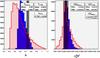 |
Fig. 4 Minimized values of h and |
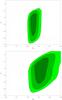 |
Fig. 5 Experimental constraints on the Galileon parameters
|
To estimate this effect, we tried to identify at which scale non-linearities start to
matter and checked whether this value is outside the range of scales taken into account in
the growth-of-structure measurements. As an example, WiggleZ measurements of
fσ8 are derived using a non-linear
growth-of-structure model (Jennings et al. 2011)
and encompass all scales k < 0.3
h Mpc-1. In this model, the frontier between the linear and
the non-linear regimes is k ≈ 0.03 h Mpc-1.
Other measurements in Table 2 include scales up to
k ≈ 0.2−0.4 h Mpc-1 as well. On the other
hand, there is no prediction in the Galileon model that goes beyond the linear regime.
However, estimates of the scale at which non-linear effects appear exist in similar
modified gravity models. Numerical simulations of the Chameleon screening effect for
 theories show that non-linearity effects can be significant at scales
k ≈ 0.05 h Mpc-1 (see Brax et al. 2012; Jennings et al. 2012 and Li et al. 2013).
Other simulations of the Vainshtein effect in the DGP model show that significant
differences between the linear and non-linear regimes appear for scales
k > 0.2 h Mpc-1
(Schmidt 2009). Unlike the DGP model, the
Galileon model we considered does not contain a direct scalar-matter coupling
~
theories show that non-linearity effects can be significant at scales
k ≈ 0.05 h Mpc-1 (see Brax et al. 2012; Jennings et al. 2012 and Li et al. 2013).
Other simulations of the Vainshtein effect in the DGP model show that significant
differences between the linear and non-linear regimes appear for scales
k > 0.2 h Mpc-1
(Schmidt 2009). Unlike the DGP model, the
Galileon model we considered does not contain a direct scalar-matter coupling
~ that is usually
considered as an essential ingredient of the Vainshtein effect. However, Babichev & Esposito-Farese (2013) showed that
even if the Galileon field is not directly coupled to matter, the cosmological evolution
of the Galileon field gives rise to an induced coupling of about 1, because of the
Galileon-metric mixing. Therefore, the Vainshtein effect is expected to operate
approximately at the same scales as in the DGP model in the model we considered.
that is usually
considered as an essential ingredient of the Vainshtein effect. However, Babichev & Esposito-Farese (2013) showed that
even if the Galileon field is not directly coupled to matter, the cosmological evolution
of the Galileon field gives rise to an induced coupling of about 1, because of the
Galileon-metric mixing. Therefore, the Vainshtein effect is expected to operate
approximately at the same scales as in the DGP model in the model we considered.
This means the lack of non-linear effects in our perturbation equations, and hence in our predictions for fσ8 in the Galileon model, is likely to have a significant impact on the constraints we derived from growth measurements, since the latter accounted partially for non-linear effects.
4.4. Full combined constraints
Results from all data are presented in Fig. 7. Table
4 presents the best-fit values for the Galileon
model parameters. The derived
value is 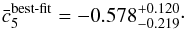 (63)Note that negative
values are preferred for the s
at the 1σ level. Moreover, the Galileon h best-fit
values are compatible with the Riess et al. (2011)
measurement.
(63)Note that negative
values are preferred for the s
at the 1σ level. Moreover, the Galileon h best-fit
values are compatible with the Riess et al. (2011)
measurement.
We carried out an a posteriori check to identify which scenarios present a significant
amount of early dark energy. At decoupling,
Ωπ(z∗) > 10%Ωr(z∗)
only for viable scenarios with 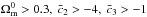 and
and
 .
This check can be made after comparing theory with data because only data can provide
values for h and . For Galileon
scenarios with
.
This check can be made after comparing theory with data because only data can provide
values for h and . For Galileon
scenarios with  ,
which is the region favoured by data, we found no significant early dark energy.
,
which is the region favoured by data, we found no significant early dark energy.
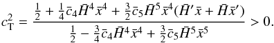
4.5. Analysis of the best-fit scenario
What does the best-fit scenario (derived from all data; the last line of Table 4) look like? Because
ρπ can be defined from the (00) Einstein
equation, a Galileon pressure Pπ can be
defined from the (ij) Einstein equation: ![Mathematical equation: \begin{eqnarray} \label{eq:ppi} \frac{P_{\pi}}{H_0^2 M_{\rm P}^2}&=& \frac{\bar c_2}{2}\h^2\x^2 + 2\bar c_3\h^3\x^2(\h \x)' - \bar c_4\left[ \frac{9}{2}\h^6\x^4 + 12 \h^6\x^3\x' \right.\nonumber \\ &&\left.\phantom{\frac{9}{2}}+ 15 \h^5\x^4\h' \right] + 3\bar c_5\h^7\x^4\left( 5\h \x' + 7\h' \x + 2\h \x \right) . \end{eqnarray}](/articles/aa/full_html/2013/07/aa21256-13/aa21256-13-eq265.png) (64)Combining
ρπ and
Pπ, an equation of state parameter
wπ(z) = Pπ(z)/ρπ(z)
can be built for the Galileon “fluid”. We can also construct an equation for
Ωπ(z) using
(64)Combining
ρπ and
Pπ, an equation of state parameter
wπ(z) = Pπ(z)/ρπ(z)
can be built for the Galileon “fluid”. We can also construct an equation for
Ωπ(z) using
 . The
evolution of wπ(z),
Ωπ(z) and
for the Galileon
best-fit scenario is shown in Figs. 8 and 9.
. The
evolution of wπ(z),
Ωπ(z) and
for the Galileon
best-fit scenario is shown in Figs. 8 and 9.
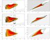 |
Fig. 6 Experimental constraints on the Galileon model from growth data (red) and from SNLS3+WMAP7+BAO+H0 combined constraints (dashed). The filled dark, medium, and light-colored contours enclose 68.3, 95.4, and 99.7% of the probability, respectively. Dark dotted regions correspond to scenarios rejected by theoretical constraints. |
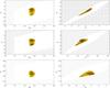 |
Fig. 7 Combined constraints on the Galileon model from SNLS3, WMAP7+BAO+H0, and growth data. The filled dark, medium, and light-yellow contours enclose 68.3, 95.4, and 99.7% of the probability, respectively. Dark dotted regions correspond to scenarios rejected by theoretical constraints. |
ΛCDM best-fit values from different data samples.
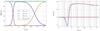 |
Fig. 8 Evolution of the Ωi(z) (left) and of w(z) (right, solid curve) for the best-fit Galileon model from all data (last row of Table 4). As a comparison, the dashed orange line gives w(z) for the best-fit scenario from SN data alone. |
4.5.1. Cosmic evolution
The left panel of Fig. 8 shows that for the best-fit scenario, radiation, matter, and dark energy (here the Galileon) dominate alternatively during the history of the Universe, as in any standard cosmological model. These three epochs are also visible in the evolution of w(z). Moreover, the best-fit scenario evolves in the future toward the de Sitter solution w = −1, which is an attractor of the Galileon model (De Felice & Tsujikawa 2010). In the region 0 < z < 1, where SNe tightly constrain dark energy, w(z) deviates significantly from − 1, its ΛCDM value. Note that in the fit with SNe alone, the deviation is less pronounced, with an average value of − 1.09 in 0 < z < 1, which is compatible with the fitted value of w in constant w dark energy models, as published in Conley et al. (2011).
During matter domination, dark energy contributes about 0.4% to the mass-energy budget
at z = 10. For comparison, in a standard ΛCDM model dark energy
contributes only 0.2% at this redshift (assuming a flat ΛCDM model with
 ).
In the same way, dark energy contributes 0.04% at z∗ in the
Galileon best-fit scenario, whereas for ΛCDM ΩΛ = 10-9 at
z∗. In our best-fit Galileon scenario, dark energy is more
present throughout the history of the Universe than in the ΛCDM model, but is still
negligible during the matter and radiation eras.
).
In the same way, dark energy contributes 0.04% at z∗ in the
Galileon best-fit scenario, whereas for ΛCDM ΩΛ = 10-9 at
z∗. In our best-fit Galileon scenario, dark energy is more
present throughout the history of the Universe than in the ΛCDM model, but is still
negligible during the matter and radiation eras.
Figure 9 shows the evolution of
for the
best-fit scenario and for the growth-data best-fit scenario. Both curves show deviations
from 1 at redshifts around 0. Particularly, the divergence near the current epoch
suggests that we should push the Galileon predictions for
fσ8 beyond the linear regime, as already
advocated in Sect. 4.3.
4.5.2. Comparison with ΛCDM
In Fig. 10 and Table 5, best-fit values for the ΛCDM parameters are presented using the
same analysis tools and observables. Interestingly, even in the ΛCDM model there is
tension between growth data and other probes. The
best-fit
value is similar in both models, but the h value departs more from the
H0Riess et al.
(2011) measurement. As far as the χ2s are
concerned, SNe Ia provide a good agreement with both models. CMB+BAO+H0 data are more
compatible with the Galileon model, reflecting the better agreement on the
h minimized value. Yet growth-of-structure data agree better with the
ΛCDM model. Finally, due to the poorer fit to growth data in the Galileon model, the
difference in χ2 is Δχ2 = 10.2.
This indicates that the Galileon model is slightly disfavored with respect to the ΛCDM
model, despite having two extra free parameters.
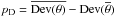
Because we are comparing two models with a different number of parameters and complexity, other criteria than comparing χ2s can be helpful. A review of the selection model criterion is provided in Liddle (2007). Because our study leads to the full computation of the likelihood functions, we can use precise criteria such as the Bayes factor (see Beringer et al. 2012; John & Narlikar 2002; Kass & Raftery 1995 and Liddle 2009) or the deviance information criterion (DIC, see Spiegelhalter et al. 2002 and Kunz et al. 2006). The Akaike information criterion (AIC) and the Bayesian information criterion (BIC) criteria used in Nesseris et al. (2010) are approximations of the first two using only the maximum likelihood and not the whole function. Hereafter we restrict the discussion to the DIC criterion.
The DIC criterion is based on the computation of the deviance likelihoods
Dev(θ) = −2log p(D|θ) + C (with
C a constant not important for DIC evaluation).
p(D|θ) is the computed likelihood function
ℒ(θ) of the model. An effective number of parameters
 is derived with
 the expectation
values for θ and
the expectation
values for θ and  the
mean deviance likelihood value:
the
mean deviance likelihood value:  (65)where
p(θ|D) is the posterior probability density
function for a vector θ of parameters of the tested model, knowing the
data D:
(65)where
p(θ|D) is the posterior probability density
function for a vector θ of parameters of the tested model, knowing the
data D:  (66)p(D),
the probability to obtain the data D, is also called the marginal likelihood because it
can be computed using the summation over all θs:
(66)p(D),
the probability to obtain the data D, is also called the marginal likelihood because it
can be computed using the summation over all θs:
 (67)Note that if the priors
are flat, p(θ|D) is just the likelihood function
ℒ(θ) normalized to 1. In our case, prior(θ) is a
flat prior reflecting the theoretically allowed volume in the scanned parameter space.
We checked that the DIC criterion is not sensitive to the exact definition of the prior,
which makes it a robust tool.
(67)Note that if the priors
are flat, p(θ|D) is just the likelihood function
ℒ(θ) normalized to 1. In our case, prior(θ) is a
flat prior reflecting the theoretically allowed volume in the scanned parameter space.
We checked that the DIC criterion is not sensitive to the exact definition of the prior,
which makes it a robust tool.
Then  . The model with the
smallest DIC is favored by the data. In our study, we obtained
DICGalileon − DICΛCDM = 12.25 > 0.
Again, the Galileon model is slightly disfavored by data against the ΛCDM model. The DIC
criterion just reflects the Δχ2 and does not penalize the
Galileon model so much because of its higher number of free parameters.
. The model with the
smallest DIC is favored by the data. In our study, we obtained
DICGalileon − DICΛCDM = 12.25 > 0.
Again, the Galileon model is slightly disfavored by data against the ΛCDM model. The DIC
criterion just reflects the Δχ2 and does not penalize the
Galileon model so much because of its higher number of free parameters.
In the future, provided the tension between growth-of-structure data and distances does not increase after more precise measurements of the observables used in this paper are included, new observables will be necessary to distinguish between the two models. A promising way would be to exploit, e.g., the ISW effect as discussed in Kobayashi et al. (2010).
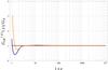 |
Fig. 9 Evolution of |
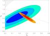 |
Fig. 10 Experimental constraints on the ΛCDM model from SNLS3 data (blue), growth data (red), BAO+WMAP7+H0 data (green), and all data combined (yellow). The black dashed line indicates the flatness condition Ωm + ΩΛ = 1. |
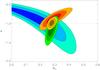 |
Fig. 11 Experimental constraints on the FWCDM model from SNLS3 data (blue), growth data (red), BAO+WMAP7+H0 data (green), and all data combined (yellow). |
FWCDM best-fit values from different data samples.
4.5.3. Comparison with FWCDM
For consistency with our assumption about flatness, we also present a comparison with the effective FWCDM model, a model with a constant dark energy equation of state parameter w in a flat Universe (see Table 6 and Fig. 11). The data set points toward a value of w below − 1, which is consistent with the Galileon best-fit scenario (see Fig. 8).
However, the difference in χ2 is the same as for the ΛCDM model, Δχ2 = 10.2, and the DIC criterion gives DICGalileon − DICFWCDM = 12.16 > 0. Here again, the Galileon model is not significantly disfavored.
5. Discussion
In this section we compare our results with other recent publications on the same subject.
Appleby & Linder (2012b) concluded that the uncoupled Galileon model is ruled out by current data since their best-fit yielded Δχ2 = 31 compared with the best-fit ΛCDM model. In addition, they obtained a long narrow region of degenerate scenarios with nearly the same likelihood. In our case, the best-fit has Δχ2 = 10.2, we obtained enclosed contours in all projections and a clear minimum.
Although we used the same expansion and perturbation equations as Appleby & Linder (2012b), there are differences between the two
works. We used a parametrization of the model, which makes our study independent of initial
conditions for x, while they set
xi = x(zi = 106)
by imposing a
ρπ(zi) which varied
in their parameter scan. This requires one to solve a fifth-order polynomial equation in
xi – and hence one is forced to choose one of the five
solutions – or to assume one of the four terms  is dominant in the (00) Einstein equation. In any case, this leads to a parameter space that
is different than the one we explored. Another difference arises from the theoretical
constraints that are used to restrict the parameter space to viable scenarios only. Our set
of theoretical constraints is larger because we also used tensorial constraints, which
proved to be very powerful. This also leads to a different explored parameter space.
is dominant in the (00) Einstein equation. In any case, this leads to a parameter space that
is different than the one we explored. Another difference arises from the theoretical
constraints that are used to restrict the parameter space to viable scenarios only. Our set
of theoretical constraints is larger because we also used tensorial constraints, which
proved to be very powerful. This also leads to a different explored parameter space.
In De Felice & Tsujikawa (2010), the
rescaling of the Galileon parameters was performed with a de Sitter solution instead of
using x0, as in this paper. This led to relations fixing their
“”
and “”
coefficients as a function of their “”
and “”
coefficients (denoted α and β in their study), but
required two initial conditions to compute the cosmological evolution. Those were also
fitted using experimental data. With this parametrization and without growth constraints,
Nesseris et al. (2010) found best-fit values for
their “”
and “”
of the same sign and same order of magnitude as in our work, despite our different
parametrizations. A second paper by Okada et al.
(2013) included redshift space distortion measurements and ruled out the Galileon
model at the 10σ level.
The first difference with respect to our work is the treatment of the initial conditions
and the use of an extra theoretical constraint to avoid numerical instabilities during the
transition from the matter era to the de Sitter epoch. This reduces the parameter space with
respect to that explored in our work. As stated above, a better modeling of
including non-linear effects should be conducted instead of discarding scenarios with such
instabilities.
Second, Okada et al. (2013) used
fσ8 measurements not corrected for the
Alcock-Paczynski effect. Moreover, to make their
fσ8 predictions in the Galileon model, Okada et al. (2013) set the normalization of
σ8 today to the WMAP7
σ8(z = 0) measurement, which was obtained in
a cosmological fit to the ΛCDM model. This normalization led to the following
σ8(z) evolution: 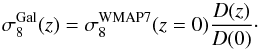 (68)This assumes that
the Galileon theory predicts a matter power spectrum similar to that of ΛCDM at
z = 0, which is not guaranteed (Barreia et
al. 2012). In contrast, we used the WMAP7 σ8
measurement to set the normalization at decoupling
z ≈ z∗ (see Eq. (59)). Thus we took into account the different
growth histories between the ΛCDM and the Galileon models (Eq. (60), which is different from Eq. (68)). We can compare our best-fit scenarios for
these two models with the fσ8 and
F measurements. Figures 12 and
13 show the result of this comparison. The agreement
with the data is good in both models. In particular, the Galileon model does not exhibit a
discrepancy as strong as was found in Fig. 3 of Okada et al.
(2013).
(68)This assumes that
the Galileon theory predicts a matter power spectrum similar to that of ΛCDM at
z = 0, which is not guaranteed (Barreia et
al. 2012). In contrast, we used the WMAP7 σ8
measurement to set the normalization at decoupling
z ≈ z∗ (see Eq. (59)). Thus we took into account the different
growth histories between the ΛCDM and the Galileon models (Eq. (60), which is different from Eq. (68)). We can compare our best-fit scenarios for
these two models with the fσ8 and
F measurements. Figures 12 and
13 show the result of this comparison. The agreement
with the data is good in both models. In particular, the Galileon model does not exhibit a
discrepancy as strong as was found in Fig. 3 of Okada et al.
(2013).
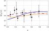 |
Fig. 12 fσ8(z) measurements from different surveys (6dFGRS, 2fFGRS, SDSS LRG, BOSS, and WiggleZ) compared with predictions for the ΛCDM model (with parameters of Table 5 – dashed purple line) Galileon scenarios. The solid blue line stands for the best-fit Galileon scenario using all data, whereas the orange dashed line stands for the best-fit Galileon scenario using growth data only. |
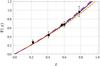 |
Fig. 13 F(z) measurements from different surveys (BOSS and WiggleZ) compared with the prediction for the ΛCDM model (with parameters of Table 5 – dashed purple line) and for Galileon scenarios. The solid blue line stands for the best-fit Galileon scenario using all data, whereas the orange dashed line stands for the best-fit Galileon scenario using growth data only. |
6. Conclusion
We have confronted the uncoupled Galileon model with the most recent cosmological data. We introduced a renormalization of the Galileon parameters by the derivative of the Galileon field normalized to the Planck mass to break some degeneracies inherent to the model. Theoretical conditions were added to restrict the analysis to viable scenarios only. This allowed us to break the parameter degeneracies that otherwise would have prevented us from obtaining enclosed probability contours. In particular, the conditions on the tensorial propagation mode of the perturbed metric proved to be very helpful.
We used a grid search technique to explore the Galileon parameter space. Our data set
encompassed the SNLS3 SN Ia sample, WMAP7
{la,R,z∗}
constraints, BAO measurements, and growth data with the Alcock-Paczynski effect taken into
account. We found  . The
final χ2 is slightly above that of the ΛCDM model due to a
poorer fit to the growth data.
. The
final χ2 is slightly above that of the ΛCDM model due to a
poorer fit to the growth data.
The best-fit Galileon scenario mimics a ΛCDM model with the three periods of radiation,
matter, and dark energy domination, with an evolving dark energy equation of state parameter
w(z), and an effective gravitational coupling
 .
Predictions for the latter are possible only in the linear regime, which may have an impact
on our results derived from growth data because the latter were computed using a non-linear
theory. A more precise theoretical and phenomenological study should be conducted to fairly
compare the Galileon model with these data.
.
Predictions for the latter are possible only in the linear regime, which may have an impact
on our results derived from growth data because the latter were computed using a non-linear
theory. A more precise theoretical and phenomenological study should be conducted to fairly
compare the Galileon model with these data.
Our best-fit is more favorable to the Galileon model than other recent results. The main difference between our treatment and those works lies in the treatment of initial conditions. We also tried to make as few assumptions and approximations as possible when computing observable quantities. Finally, when using growth data, we took care to choose measurements that were derived in a model-independent way. In the future, a study considering precise predictions of the full power spectra as suggested by Barreia et al. (2012) would provide more stringent tests of the validity of the Galileon model.
If the optional coupling parameters c0 and
cG are included, they should be redefined
as  and
and  . But if
c0 ≠ 0, two initial conditions are needed
(π0 and
. But if
c0 ≠ 0, two initial conditions are needed
(π0 and  ). With our
new parametrization we would have to introduce and fit a new parameter
). With our
new parametrization we would have to introduce and fit a new parameter
 .
.
Acknowledgments
We thank Philippe Brax for introducing us to the Galileon theory, and Christos Charmoussis, Cédric Deffayet, Jean-Baptiste Melin, and Marc Besançon for fruitful discussions about the Galileon model. We also thank Chris Blake for useful advice on the use of the WiggleZ measurements. The work of Eugeny Babichev was supported in part by grant FQXi-MGA-1209 from the Foundational Questions Institute.
References
- Alcock, C., & Paczynski, B. 1979, Nature, 281, 358 [NASA ADS] [CrossRef] [Google Scholar]
- Anderson, L., Aubourg, E., Bailey, S., et al. 2012, MNRAS, 427, 3435 [Google Scholar]
- Appleby, S. A., & Linder, E. 2012a, JCAP, 1203, 44 [Google Scholar]
- Appleby, S. A., & Linder, E. 2012b, JCAP, 08, 26 [NASA ADS] [CrossRef] [Google Scholar]
- Astier, P., Guy, J., Regnault, N., et al. 2006, A&A, 447, 31 [NASA ADS] [CrossRef] [EDP Sciences] [Google Scholar]
- Babichev, E., & Esposito-Farese, G. 2013, Phys. Rev. D, 87, 044032 [NASA ADS] [CrossRef] [Google Scholar]
- Babichev, E., Deffayet, C., Esposito-Farese, G. 2011, Phys. Rev. Lett., 107, 251102 [NASA ADS] [CrossRef] [PubMed] [Google Scholar]
- Barreira, A., Li, B., Baugh, C. M., et al. 2012, Phys. Rev. D, 86, 124016 [NASA ADS] [CrossRef] [Google Scholar]
- Beutler, F., Blake, C., Colless, M., et al. 2011, MNRAS, 416, 3017 [NASA ADS] [CrossRef] [Google Scholar]
- Beutler, F., Blake, C., Colless, M., et al. 2012, MNRAS, 423, 3430 [NASA ADS] [CrossRef] [Google Scholar]
- Beringer, J., Arguin, J.-F., Barnett, R. M., et al. (Particle Data Group) 2012, Phys. Rev. D, 86, 010001 [Google Scholar]
- Blake, C., Brough, S., Colless, M., et al. 2011a, MNRAS, 415, 2876 [NASA ADS] [CrossRef] [Google Scholar]
- Blake, C., Glazebrook, K., Davis, T. M., et al. 2011b, MNRAS, 418, 1725 [NASA ADS] [CrossRef] [Google Scholar]
- Brax, P., Burrage, C., & Davis, A.-C. 2011, JCAP, 020, 1109 [Google Scholar]
- Brax, P., Davis, A.-C., Li, B., et al. 2012, JCAP, 10, 002 [Google Scholar]
- Burrage, C., & Seery, D. 2010, JCAP, 08, 011 [NASA ADS] [CrossRef] [Google Scholar]
- Conley, A., Guy, J., Sullivan, M., et al. 2011, ApJS, 192, 1 [NASA ADS] [CrossRef] [EDP Sciences] [Google Scholar]
- De Felice, A., & Tsujikawa, S. 2010, Phys. Rev. Lett., 105, 111301 [NASA ADS] [CrossRef] [Google Scholar]
- De Felice, A., & Tsujikawa, S. 2011, Phys. Rev. D, 84, 124029 [NASA ADS] [CrossRef] [Google Scholar]
- Deffayet, C., Esposito-Farese, G., & Vikman, A. 2009, Phys. Rev. D, 79, 084003 [NASA ADS] [CrossRef] [Google Scholar]
- Dvali, G. R., Gabadadze, G., & Porrati, M. 2000, Phys. Lett. B, 485, 208 [NASA ADS] [CrossRef] [MathSciNet] [Google Scholar]
- Eisenstein, D. J., & Hu, W. 1998, ApJ, 496, 605 [NASA ADS] [CrossRef] [Google Scholar]
- Eisenstein, D. J., Zehavi, I., Hogg, D. W., et al. 2005, ApJ, 633, 650 [Google Scholar]
- Faraoni, V., Gunzig, E., & Nardone, P. 1999, Fund. Cosmic Phys., 20, 121 [NASA ADS] [Google Scholar]
- Guy, J., Astier, P., Baumont, S., et al. 2007, A&A, 466, 11G [NASA ADS] [CrossRef] [EDP Sciences] [Google Scholar]
- Guy, J., Sullivan, M., Conley, A., et al. 2010, A&A, 523, A7 [NASA ADS] [CrossRef] [EDP Sciences] [Google Scholar]
- Horndeski, G. W. 1974, Int. J. Theor. Phys., 10, 363 [CrossRef] [MathSciNet] [Google Scholar]
- Hu, W., & Sugiyama, N. 1996, ApJ, 471, 542 [NASA ADS] [CrossRef] [Google Scholar]
- Jennings, E., Baugh, C. M., & Pascoli, S. 2011, MNRAS, 410, 2081 [NASA ADS] [Google Scholar]
- Jennings, E., Baugh, C. M., Li, B., et al. 2012, MNRAS, 425, 2128 [NASA ADS] [CrossRef] [Google Scholar]
- John, M. V., & Narlikar, J. V. 2002, Phys. Rev. D, 65, 043506 [NASA ADS] [CrossRef] [MathSciNet] [Google Scholar]
- Kass, R. E., & Raftery, A. E. 1995, J. Am. Stat. Assoc., 90:430, 773 [Google Scholar]
- Kobayashi, T., Tashiro, H., & Suzuki, D. 2010, Phys. Rev. D, 81, 063513 [NASA ADS] [CrossRef] [Google Scholar]
- Komatsu, E., Dunkley, J., Nolta, M. R., et al. 2009, ApJS, 180, 330 [NASA ADS] [CrossRef] [Google Scholar]
- Komatsu, E., Smith, K. M., Dunkley, J., et al. 2011, ApJS, 192, 18 [NASA ADS] [CrossRef] [Google Scholar]
- Kunz, M., Trotta, R., & Parkinson, D. 2006, Phys. Rev. D, 74, 023503 [NASA ADS] [CrossRef] [MathSciNet] [Google Scholar]
- Lewis, A., & Bridle, S. 2002, Phys. Rev. D, 66, 103511 [NASA ADS] [CrossRef] [Google Scholar]
- Li, B., Hellwing, W. A., Koyama, K., et al. 2013, MNRAS, 428, 743 [NASA ADS] [CrossRef] [Google Scholar]
- Liddle, A. R. 2007, MNRAS, 377, 74 [Google Scholar]
- Liddle, A. R. 2009, Ann. Rev. Nucl. Part. Sci., 114, 29 [Google Scholar]
- Linder, E. 2005, Phys. Rev. D, 72, 043529 [NASA ADS] [CrossRef] [MathSciNet] [Google Scholar]
- Mangano, G., Miele, G., Pastor, S., et al. 2002, Phys. Lett. B, 534, 8 [NASA ADS] [CrossRef] [Google Scholar]
- Nesseris, S., De Felice, A., & Tsujikawa, S. 2010, Phys. Rev. D, 82, 124054 [NASA ADS] [CrossRef] [Google Scholar]
- Nicolis, A., Rattazzi, R., & Trincherini, E. 2009, Phys. Rev. D, 79, 064036 [NASA ADS] [CrossRef] [MathSciNet] [Google Scholar]
- Okada, H., Totani, T., & Tsujikawa, S. 2013, Phys. Rev. D, 87, 103002 [Google Scholar]
- Padmanabhan, N., Xu, X., Eisenstein, D. J., et al. 2012, MNRAS, 427, 2132 [NASA ADS] [CrossRef] [MathSciNet] [Google Scholar]
- Percival, W. J., Burkey, D., Heavens, A., et al. 2004, MNRAS, 353, 1201 [NASA ADS] [CrossRef] [Google Scholar]
- Perlmutter, S., Aldering, G., Goldhaber, G., et al. 1999, ApJ, 517, 565 [NASA ADS] [CrossRef] [Google Scholar]
- Regnault, N., Conley, A., Guy, J., et al. 2009, A&A, 506, 999 [NASA ADS] [CrossRef] [EDP Sciences] [Google Scholar]
- Reid, B. A., Samushia, L., White, M., et al. 2012, MNRAS, 426, 2719 [NASA ADS] [CrossRef] [Google Scholar]
- Riess, A. G., Filippenko, A. V., Challis, P., et al. 1998, AJ, 116, 1009 [NASA ADS] [CrossRef] [Google Scholar]
- Riess, A. G., Macri, L., Casertano, S., et al. 2011, ApJ, 730, 119 [NASA ADS] [CrossRef] [Google Scholar]
- Samushia, L., Percival, W. J., & Raccanelli, A. 2012a, MNRAS, 420, 2102 [NASA ADS] [CrossRef] [Google Scholar]
- Samushia, L., Reid, B. A., White, M., et al. 2012b, MNRAS, 1093, 10 [Google Scholar]
- Sánchez, A. G., Scóccola, C. G., Ross, A. J., et al. 2012, MNRAS, 425, 415 [NASA ADS] [CrossRef] [Google Scholar]
- Schmidt, F. 2009, Phys. Rev. D, 80, 123003 [NASA ADS] [CrossRef] [Google Scholar]
- Song, Y. S., & Percival, W. 2009, JCAP, 0910, 004 [NASA ADS] [CrossRef] [Google Scholar]
- Spiegelhalter, D. J., Best, N. G., Carlin, B. P., et al. 2002, J. Roy. Statist. Soc. B., 64.4, 583 [Google Scholar]
- Sullivan, M., Guy, J., Regnault, N., et al. 2011, ApJ, 737, 102 [NASA ADS] [CrossRef] [Google Scholar]
- Trodden, M., & Hinterbichler, K. 2011, Class. Quant. Grav, 28, 204003 [Google Scholar]
- Vainshtein, A. I. 1972, Phys. Lett. B, 39, 396 [NASA ADS] [CrossRef] [Google Scholar]
Appendix A: Instability of probability contours
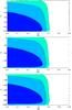 |
Fig. A.1 Experimental constraints on the Galileon model from SNLS3 data for different ranges
in cis using the method developed in Appendix A, with
α and β fixed to their ΛCDM best-fit values from
Sullivan et al. (2011). The
four-dimensional likelihood |


Instead of absorbing the initial condition x0 in the
 redefinition, we can be tempted to fix it using the (00) Einstein equation at
z = 0 for each scenario:
redefinition, we can be tempted to fix it using the (00) Einstein equation at
z = 0 for each scenario: 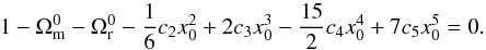 (A.1)To find
x0, a fifth-order polynomial equation is to be solved, which
can lead to five complex solutions. A reasonable choice is to keep only the scenarios that
give a unique real solution.
(A.1)To find
x0, a fifth-order polynomial equation is to be solved, which
can lead to five complex solutions. A reasonable choice is to keep only the scenarios that
give a unique real solution.
 |
Fig. A.2 Left panel: evolution of la with amin without the linear interpolation as described in the text for a subset of Galileon scenarios. Note that most scenarios approach the WMAP7 measurement la ≈ 300. Right panel: correction to la for different values of amin and for the same subset of scenarios as in the left panel. The dashed line is the value of σla, the WMAP7 measurement error on la. |
The system of differential Eqs. (8) and (9) adopts an unusual behavior. Referring to Fig. A.1, the shape of the probability contours remains unchanged regardless of the limits of the scanned parameter space. In other words, the likelihood surface is invariant when the limits of the explored parameter space are proportionally changed. The model seems to exhibit a scale invariance allowing data to be fitted regardless of the boundaries of the explored parameter range. Moreover, we cannot obtain contours well enclosed in any explored parameter space: the likelihood surface has an infinite valley of minimum χ2 instead of a unique minimum.
Equation (A.1) shows that small
cis produce a high x0, and high
cis a low x0. Nevertheless, the
theoretical constraints of Sect. 2.5 cannot favor or
disfavor high cis or x0 because
they also contain this correspondence between the cis and
x0. Accordingly, for different sets of
cis, identical cosmological scenarios are computed
regardless of the scale of the cis: the important point is
that these equivalent scenarios have the same
Ωπ(z), whether this is due to high or small
cis and as a consequence have the same
evolution and then the same χ2.
Thus, a scale choice has to be made to fix the likelihood surface, but this choice has
not to be arbitrary. A solution is provided in 2.2 by
absorbing x0 into new parameters
s.
This new parametrization absorbs a degree of freedom and allows us to use the (00)
Einstein equation to fix .
This may be the origin of the degeneracy in χ2 reported in
Sect. III of Appleby & Linder (2012a).
Appendix B: Approximation for la computation
The computation of la (see Eq. (42)) requires the evolution of the cosmological model from today to a = 0 (see Eq. (40)). In the Galileon context, the non-linear evolution equations require increasing precision and finer steps when approaching the limit a → 0. In addition, it is physically questionable to extrapolate the Galileon model up to the very first instants of the Universe.
Therefore our iterative computation is stopped at a certain
amin close to 0, without affecting significantly the final
value of la. Let amin − 1 be the
step before amin where the cosmological equations are
computed, and f(a) the integrand function of
rs(z∗). Although the integral is
stopped at a = amin, we can compensate this
approximation by a linear interpolation of the integral:
 (B.1)In
the left panel of Fig. A.2, we present the evolution
of la with amin without the linear
interpolation for a subset of Galileon scenarios. The smooth evolution with
amin allows us to consider the linear interpolation as a
reasonable assumption. Moreover, for amin ≲ 10-6,
the value of la changes less than the WMAP7 measurement error
σla = 0.76, as shown in the
right panel of Fig. A.2. Based on these results, we
decide to use amin = 10-7, which provides a
correction on la an order of magnitude below
σla.
(B.1)In
the left panel of Fig. A.2, we present the evolution
of la with amin without the linear
interpolation for a subset of Galileon scenarios. The smooth evolution with
amin allows us to consider the linear interpolation as a
reasonable assumption. Moreover, for amin ≲ 10-6,
the value of la changes less than the WMAP7 measurement error
σla = 0.76, as shown in the
right panel of Fig. A.2. Based on these results, we
decide to use amin = 10-7, which provides a
correction on la an order of magnitude below
σla.
All Tables
All Figures
|
Fig. 1 Confidence contours for the SN nuisance parameters α and β when marginalizing over all other parameters of the model. Dashed red contours represent 68.3%, 95.4%, and 99.7% probability contours for the ΛCDM model. Filled blue contours are for the Galileon model. Note that they are nearly identical, the Galileon one is just 2.8% wider, which is likely due to larger steps in α and β. See Table 3 for numerical values. |
| In the text | |
|
Fig. 2 Experimental constraints on the Galileon model from SNLS3 data alone. To
represent the four-dimensional likelihood |
| In the text | |
|
Fig. 3 Experimental constraints on the Galileon model from WMAP7+BAO+H0 data. To
represent the four-dimensional likelihood |
| In the text | |
|
Fig. 4 Minimized values of h and |
| In the text | |
|
Fig. 5 Experimental constraints on the Galileon parameters
|
| In the text | |
|
Fig. 6 Experimental constraints on the Galileon model from growth data (red) and from SNLS3+WMAP7+BAO+H0 combined constraints (dashed). The filled dark, medium, and light-colored contours enclose 68.3, 95.4, and 99.7% of the probability, respectively. Dark dotted regions correspond to scenarios rejected by theoretical constraints. |
| In the text | |
|
Fig. 7 Combined constraints on the Galileon model from SNLS3, WMAP7+BAO+H0, and growth data. The filled dark, medium, and light-yellow contours enclose 68.3, 95.4, and 99.7% of the probability, respectively. Dark dotted regions correspond to scenarios rejected by theoretical constraints. |
| In the text | |
|
Fig. 8 Evolution of the Ωi(z) (left) and of w(z) (right, solid curve) for the best-fit Galileon model from all data (last row of Table 4). As a comparison, the dashed orange line gives w(z) for the best-fit scenario from SN data alone. |
| In the text | |
|
Fig. 9 Evolution of |
| In the text | |
|
Fig. 10 Experimental constraints on the ΛCDM model from SNLS3 data (blue), growth data (red), BAO+WMAP7+H0 data (green), and all data combined (yellow). The black dashed line indicates the flatness condition Ωm + ΩΛ = 1. |
| In the text | |
|
Fig. 11 Experimental constraints on the FWCDM model from SNLS3 data (blue), growth data (red), BAO+WMAP7+H0 data (green), and all data combined (yellow). |
| In the text | |
|
Fig. 12 fσ8(z) measurements from different surveys (6dFGRS, 2fFGRS, SDSS LRG, BOSS, and WiggleZ) compared with predictions for the ΛCDM model (with parameters of Table 5 – dashed purple line) Galileon scenarios. The solid blue line stands for the best-fit Galileon scenario using all data, whereas the orange dashed line stands for the best-fit Galileon scenario using growth data only. |
| In the text | |
|
Fig. 13 F(z) measurements from different surveys (BOSS and WiggleZ) compared with the prediction for the ΛCDM model (with parameters of Table 5 – dashed purple line) and for Galileon scenarios. The solid blue line stands for the best-fit Galileon scenario using all data, whereas the orange dashed line stands for the best-fit Galileon scenario using growth data only. |
| In the text | |
|
Fig. A.1 Experimental constraints on the Galileon model from SNLS3 data for different ranges
in cis using the method developed in Appendix A, with
α and β fixed to their ΛCDM best-fit values from
Sullivan et al. (2011). The
four-dimensional likelihood |
| In the text | |
|
Fig. A.2 Left panel: evolution of la with amin without the linear interpolation as described in the text for a subset of Galileon scenarios. Note that most scenarios approach the WMAP7 measurement la ≈ 300. Right panel: correction to la for different values of amin and for the same subset of scenarios as in the left panel. The dashed line is the value of σla, the WMAP7 measurement error on la. |
| In the text | |
Current usage metrics show cumulative count of Article Views (full-text article views including HTML views, PDF and ePub downloads, according to the available data) and Abstracts Views on Vision4Press platform.
Data correspond to usage on the plateform after 2015. The current usage metrics is available 48-96 hours after online publication and is updated daily on week days.
Initial download of the metrics may take a while.