| Issue |
A&A
Volume 555, July 2013
|
|
|---|---|---|
| Article Number | A13 | |
| Number of page(s) | 11 | |
| Section | Interstellar and circumstellar matter | |
| DOI | https://doi.org/10.1051/0004-6361/201220691 | |
| Published online | 19 June 2013 | |
Diffusion measurements of CO, HNCO, H2CO, and NH3 in amorphous water ice
1 Aix-Marseille Université, CNRS, PIIM, UMR 7345, 13013 Marseille, France
e-mail: This email address is being protected from spambots. You need JavaScript enabled to view it.
2 Academia Sinica, Institute of Astronomy and Astrophysics, Astronomy-Mathematics Building, NTU, 10617 Taipei, R.O.C., Taiwan
Received: 5 November 2012
Accepted: 2 May 2013
Abstract
Context. Water is the major component of the interstellar ice mantle. In interstellar ice, chemical reactivity is limited by the diffusion of the reacting molecules, which are usually present at abundances of a few percent with respect to water.
Aims. We want to study the thermal diffusion of H2CO, NH3, HNCO, and CO in amorphous water ice experimentally to account for the mobility of these molecules in the interstellar grain ice mantle.
Methods. In laboratory experiments performed at fixed temperatures, the diffusion of molecules in ice analogues was monitored by Fourier transform infrared spectroscopy. Diffusion coefficients were extracted from isothermal experiments using Fick’s second law of diffusion.
Results. We measured the surface diffusion coefficients and their dependence with the temperature in porous amorphous ice for HNCO, H2CO, NH3, and CO. They range from 10-15 to 10-11 cm2 s-1 for HNCO, H2CO, and NH3 between 110 K and 140 K, and between 5–8 × 10-13 cm2 s-1 for CO between 35 K and 40 K. The bulk diffusion coefficients in compact amorphous ice are too low to be measured by our technique and a 10-15 cm2 s-1 upper limit can be estimated. The amorphous ice framework reorganization at low temperature is also put in evidence.
Conclusions. Surface diffusion of molecular species in amorphous ice can be experimentally measured, while their bulk diffusion may be slower than the ice mantle desorption kinetics.
Key words: astrochemistry / molecular processes / ISM: molecules
© ESO, 2013
1. Introduction
Infrared observations of molecular clouds have proven that H2O is the most abundant solid-state molecule in the interstellar ice mantle (Whittet et al. 1983; Boogert et al. 2004, 2008a; Gibb et al. 2004; Dartois 2005; Knez et al. 2005). Thus, it is clear that the presence of water ice on the grain surface will have a major influence on the grain chemistry. The most straightforward influence is the need for the reacting species to diffuse in water ice before reacting, which leads to a diffusion-limited reactivity in interstellar ice.
Most of the gas-grain chemistry deterministic models take the diffusion of the reactants into account by correcting the chemical reaction rate following the formalism proposed by Hasegawa et al. (1992). In this formalism the chemical reaction rate is corrected by a diffusion factor based on both the thermal hopping and quantum tunneling probabilities of an adsorbed species to migrate on an adjacent surface site. The thermal hopping rate is calculated following an Arrhenius law, considering a pre-exponential factor corresponding to a characteristic vibration frequency (1012–1013 s-1), and an activation energy for diffusion equal to a third of the activation energy for desorption, following Tielens & Allamandola (1987). However, no experimental study exists to benchmark this diffusion formalism, though it is widely used in many gas-grain codes. In order to benchmark the diffusion-limited reactivity formalism, we shall start our study by measuring only the diffusion coefficients for each reactant independently. In a following work, the reactivity will be added to the diffusion.
The bulk diffusion in crystalline ice and the surface diffusion on crystalline ice have been measured for several molecular species (e.g. Livingston et al. 2002 and references therein). Bulk diffusion is thought to be governed by a vacancy-sites migration mechanism with typical diffusion coefficients D from 10-13 to 10-10 cm2 s-1 for a temperature range between 140 K and 200 K. However, extrapolating Livingston et al. (2002) data to lower temperatures would lead to an impossibility for large molecules to diffuse in crystalline ice. For example CH3OH would have a diffusion coefficient of 10-26 cm2 s-1 at 100 K, and would diffuse across 100 nm in 104 years. Diffusion in amorphous ice has also been put into evidence by Smith et al. (1997a), where the amorphous solid water (ASW) is shown to exhibit a liquid-like translational diffusion, 106±1 times faster than diffusion in crystalline ice. However, very few studies on molecule diffusion in ASW exist, while interstellar ice is observed to be amorphous (Jenniskens et al. 1995).
In this study, we have measured the kinetic rates of diffusion for several astrophysically relevant molecules in interstellar ice analogues. In Sect. 2, we summarize experimental details. In Sect. 3 we measure the relaxation or reorganization time of our interstellar ASW ice analogues at several temperatures, and we measure the diffusion coefficients for CO, HNCO, H2CO, and NH3. These species have different physical properties (mass, van der Waals radius, dipole moment, polarizability, number of hydrogen bonds) and therefore interact with the ice substrate differently. Both bulk (or volume) diffusion within the ASW ice and surface diffusion on the effective area of the ASW ice coexist, and they have different diffusion coefficients. In order to disentangle these two types of diffusion, we have worked on two extreme cases: (i) a compact non-porous amorphous ice where bulk diffusion through the ice dominates and (ii) a porous amorphous ice where surface diffusion dominates along cracks and pores. In compact amorphous ice the bulk diffusion coefficients of the molecules are too small to be measured using our technique, so we can only set an upper limit of 10-15 cm2 s-1 to bulk diffusion for the temperature range investigated. In porous amorphous ice, we have measured the surface diffusion between 35 K and 140 K for CO, HNCO, H2CO, and NH3. We have used a propagation equation to derive the diffusion coefficients for each molecule. We show that the reorganization and the crystallization of the substrate from amorphous ice to crystalline ice are concomitant with the diffusion, and may affect the diffusion of the species on a moving ASW ice network (Jenniskens & Blake 1994; Jenniskens et al. 1995; Hodyss et al. 2008; Öberg et al. 2009). Nevertheless, the contribution of the diffusion induced by the phase change on the overall surface diffusion is hard to quantify. The astrophysical implication of the diffusion on the ice mantle reactivity is then discussed in Sect. 4.
2. Experimental
2.1. The experimental set-up
The experiments were performed using our RING experimental set-up as described elsewhere (Theulé et al. 2011). A gold-plated copper surface is maintained at low temperature using a closed-cycle helium cryostat (ARS Cryo, model DE-204 SB, 4 K cryogenerator) within a high-vacuum chamber at a few 10-9 mbar. The infrared spectra are recorded by means of Fourier-transform reflection absorption infrared spectroscopy (or FTIR) using a Vertex 70 spectrometer with either a DTGS detector or a liquid N2 cooled MCT detector. A typical spectrum has a 1 cm-1 resolution and is averaged over a few tens of interferograms. The sample temperature is measured with a DTGS 670 Silicon diode with a 0.1 K uncertainty. The temperature is controlled using a Lakeshore Model 336 temperature controller and a heating resistance.
Gas-phase CO, NH3, and H2O are inserted and outgassed into a vacuum line using standard manometric techniques. The H2CO molecule is obtained by gently warming paraformaldehyde. The HNCO monomer is synthesized from the thermal decomposition of the cyanuric acid polymer (Aldrich Chemical Co., 98%) at 650 °C under a primary vacuum (Mispelaer et al. 2012). Water vapor is obtained from deionized water which has been purified by several freeze-pump-thaw cycles, carried out under a primary vacuum. Room temperature gas-phase molecules are then sprayed onto the gold surface.
2.2. The experimental protocol
The experimental protocol is to deposit, at normal incidence, a thin layer of the species on the gold plate and then to deposit a much thicker layer, of thickness d, of amorphous solid water on top of the first layer as displayed in Fig. 1.
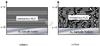 |
Fig. 1 Scheme of the bilayer sample: a thin layer of the studied M molecule (M being CO, HNCO, H2CO, or NH3) is first deposited at 15 K on the gold surface, and then a thicker layer of ASW ice is deposited on top of it at 15 K. The thickness d of the ASW layer is estimated both using H2O IR absorption bands and by interferometry. The diffusion of the M molecule along the x direction is monitored at a fixed temperature by recording the evolution of one of its characteristic IR absorption bands as function of time using FTIR spectroscopy. A compact ASW ice favors a bulk (volume) diffusion (left part), while a porous ASW ice favors a surface diffusion along cracks and pores (surface). |
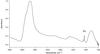 |
Fig. 2 Infrared spectrum of a NH3:ASW bilayer film at 15 K. The quantity of deposited NH3 and H2O are derived from their characteristic absorption bands. The diffusion of NH3 along the x direction at a fixed temperature T will be monitored by recording the decay of its characteristic absorption band at 1110 cm-1 as a function of time. |
The morphology of the ASW ice depends on the temperature of the gold surface the water vapor is deposited on. If the water ice is deposited at a low temperature, around 15 K, the ice film is amorphous and porous (Mayer & Pletzer 1986). Small OH dangling bands are visible at 3494 and 3480 cm-1, indicating a large effective surface and porosity (Rowland et al. 1991; Manca et al. 2002). Once slightly warmed up these dangling bands quickly disappear, indicating the start of the pore collapse and the decrease of the effective surface. However, if the water ice is deposited at a temperature ranging from 90 K and 150 K, the ice is amorphous and compact. If deposited above 150 K, the ice is crystalline. The deposition temperature, therefore, allows us to approximately choose the volume : surface ratio. However, since we can neither control nor measure this ratio, we will only work on two extreme cases: the highly porous ice, deposited at 15 K, with a large effective area, and the compact ice, deposited at 100 K, with a dominant volume component. In this work we will focus only on amorphous ice since interstellar ice is amorphous (Jenniskens et al. 1995).
The quantity of each molecular species is derived right after deposition from the IR spectra of the bilayer film, as seen in Fig. 2. The characteristic bands of each molecule are integrated, and then divided by their corresponding band strengths to estimate their column densities N (molecules cm-2). The characteristic band frequencies and band strengths for each molecule are summarized in Table 1. There is an approximate 30% uncertainty on the band strengths (derived from transmission experiments) and, therefore, on the calculated column densities.
After deposition, the ice bilayer is then heated to a fixed temperature T. Once temperature T is reached, we set t = 0 s. Then, the M molecules diffuse in the water ice film, eventually reach the surface of the ice, and desorb. The diffusion of M along the x direction at the fixed temperature T is monitored by recording the decay of its characteristic absorption band as a function of time. Figure 3 shows an isothermal time decay curve for the M = NH3 abundance at the fixed temperature of 115 K, monitored by IR spectroscopy on the NH3 characteristic absorption band at 1110 cm-1. The IR decay curve is directly related to the NH3 molecule diffusion in the porous ASW ice.
At t = 0 s, all the M molecules should be located at the bottom of the ASW layer (x = 0). If this assumption were correct, it should take some time before the first molecules reach the surface of the ice and so the abundance should remain at its maximum for a certain amount of time. As seen in Fig. 3, an abundance plateau of this kind is not observed, meaning that the diffusion has already started before t = 0 (while the film is being warmed to the fixed temperature T). Thus, it is more reasonable to assume that the two species are homogeneously mixed at t = 0: n(x,t = 0) = n0, where n(x,t) is the density of the M molecules.
Frequency positions and integrated band strengths of solid-state molecules at 10 K.
At t ≥ 0, the M molecules are diffusing into the ASW layer. Since the ice sample can be represented by a cylinder of a few centimeters in diameter and a few hundred nanometers in thickness, we can reasonably assume that the M molecules are mainly propagating along the x direction within the ASW layer and that a negligible amount of them escape from the cylinder side. The M molecules diffuse in the water ice film and desorb once they have reached the top surface of the ice. Recording the time decay of the M molecules characteristic IR absorption band enables us to monitor its diffusion in the ASW film. We therefore have two sequential phenomena: the diffusion in the ASW film, and the desorption from the top surface to the gas phase. To avoid dealing with both phenomena, we eliminate the desorption process by working at a temperature high enough that the desorption timescale is much shorter than the diffusion timescale. The residence time of each molecule is independently measured prior to diffusion experiments at different temperatures to set the lower limit temperature at which the desorption process can be neglected. In that case, the desorption kinetics do not need to be taken into account in our study and the time decay we measure is essentially a diffusion time. The accretion rate of water from background gas is estimated to be lower than 1.4 monolayer per hour, which is roughly less than a tenth of the initial ice thickness.
The upper temperature range of this technique is limited by the ASW desorption time and the instrumental time to acquire a few spectra. The lower temperature range of this technique is limited by the choice of keeping a diffusion time much longer than the residence time of the molecule M on the ASW ice surface to avoid taking desorption into account. In practice the diffusion timescale corresponds to 102 to 106 s. For a ASW thickness of few hundred layers, this time interval corresponds to diffusion coefficients of 10-15 cm2 s-1 to 10-11 cm2 s-1, which corresponds to a certain temperature range according to the molecule. Another time constraint is added if the molecule is reacting with H2O, as it is the case for H2CO forming HOCH2OH (Noble et al. 2012) and for HNCO forming H3O+OCN− (Theulé et al. 2011).
The dispersion on the diffusion coefficients is evaluated by repeating the same experiment on NH3 at 117 K five times, and applied to all the molecules.
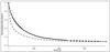 |
Fig. 3 Isothermal diffusion of NH3 through a porous ASW layer at 115 K. Markers: experimental IR decay curve sexp(t) of NH3. Theoretical curve sfl(t) using the Fick’s second law for diffusion (dashed line). Theoretical curve sfl(t) using the Avrami equation (solid line). |
2.3. Determination of the ASW film thickness
The ASW ice film thickness d through which the M molecules need to diffuse is an important parameter in our experiment. We measure it using two different methods.
The first method is based on the quantity of matter determined from the IR spectrum, using H2O stretching, bending, and libration mode IR absorption bands. The ASW thickness d is derived from the measured column density N (molecules cm-2) using ρ = 0.94 g cm-3 as the amorphous ice density, and using ![Mathematical equation: \begin{equation} \label{thickness1} d_{\rm [cm]}= \frac{N\times 18}{\rho\times N_{\rm A}}\times\frac{\cos\alpha}{2}, \end{equation}](/articles/aa/full_html/2013/07/aa20691-12/aa20691-12-eq45.png) (1)where NA is the Avogadro number, 18 g mol-1 is the molar mass for H2O, and α (18° in our case) is the incidence angle of the IR beam on the surface. The uncertainty on the ASW thickness is therefore mainly given by the uncertainty on the band strengths. The ASW thickness can be expressed in units of monolayers (ML) by dividing the column density N (molecules cm-2) by a typical 1.1 × 10¹⁵ molecules cm-2 ML-1 surface density.
(1)where NA is the Avogadro number, 18 g mol-1 is the molar mass for H2O, and α (18° in our case) is the incidence angle of the IR beam on the surface. The uncertainty on the ASW thickness is therefore mainly given by the uncertainty on the band strengths. The ASW thickness can be expressed in units of monolayers (ML) by dividing the column density N (molecules cm-2) by a typical 1.1 × 10¹⁵ molecules cm-2 ML-1 surface density.
The second method of determining the ice film thickness d is to use optical interferometry (Zondlo et al. 1997) during the ASW film deposition performed at 15 K and at a water partial pressure of 10-6 mbar. A He-Ne laser beam is incident on the growing ice film at θ1 = 36° from the surface normal and is detected with a photodiode. Using the Snell-Descartes law, the ASW ice film thickness d can be expressed using 2n2dcosθ2 = mλ, with n1 = 1 and n2 = 1.31 the refractive indices for vacuum and ice at 632.8 nm, respectively, and θ2 the refracted angle of the He-Ne beam within the ASW thickness. We can calculate that d1 = 270 nm corresponds to one interference fringe. During the deposition of the ASW film thickness, at time t, the thickness d(t) can be related to the photodiode signal sph(t) by 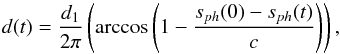 (2)where c is the contrast, i.e., the signal difference between complete constructive and destructive interferences. Figure 4 shows a typical interference pattern obtained during deposition.
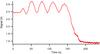 |
Fig. 4 He-Ne laser interference fringes pattern obtained during the ASW film deposition at 15 K. |
The photodiode signal position on the interference fringes pattern of Fig. 4 gives us a measurement of the ASW film thickness. The poor quality of the interference pattern is mainly due to the low power of the He-Ne laser. We stop the ASW deposition at the desired ASW film thickness, which we will call d. A comparison between the thicknesses derived using the two techniques will be made later in Sect. 3.1.2.
3. Results and discussion
The experimental protocol described above has been applied to measure the diffusion of CO, HNCO, H2CO, and NH3, both in compact and porous amorphous ice. Before presenting the results on the diffusion of the different molecules, it is important to first study the ASW ice itself, and particularly its reorganization.
3.1. Amorphous ice reorganization
The possible relationship between diffusion and the amorphous-to-crystalline ice phase change has been dealt with by Jenniskens & Blake (1994); Jenniskens et al. (1995) or Hodyss et al. (2008); Öberg et al. (2009). To understand the possible link between the diffusion and the ice relaxation, we need to investigate the ASW reorganization, as it leads to a compaction and a change in porosity of the ice.
3.1.1. Measurement of the ASW ice film reorganization rate
The ASW ice IR spectrum evolves with time, and thus we need to investigate its reorganization rate. The ASW ice to crystalline ice kinetics has been studied on 100 ML films (Smith et al. 2011) and on interstellar ice analogues (Baragiola et al. 2009) for temperatures down to 135 K using an Avrami equation 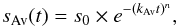 (3)where kAv is a rate constant (in s-1). The Avrami equation usually describes how solids transform from one phase to another at a constant temperature (Avrami 1939, 1940, 1941). It can describe a kinetics of crystallization, but it can apply more generally to other phase change of materials or chemical reactions. There is no clear physical interpretation of the n Avrami parameter, which is an integer varying between 1 and 4, and is related to the nature of the transformation. For a homogeneous three-dimension growth, the value of 4 is usually adopted.
Smith et al. (2011) derived a crystallization rate constant of kcryst = (1.2 ± 0.5) × 1021 s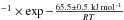 using IR spectroscopy (and (7.3 ± 2.6) × 1021 s
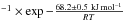 using temperature programmed desorption experiments), while Baragiola et al. (2009) derived a 59.4 ± 2.2 kJ mol-1 crystallization activation energy on a 300 nm thick ice films. Since the pre-exponential factor is not reported in Baragiola et al. (2009) it is not possible to comment on the small difference in the crystallization activation energy. Moreover, Mate et al. (2012) found that if the crystallization rate constants for ASW ice deposited at different temperatures were the same, the Avrami n parameters would be different, close to 1 for ice samples generated at 14 K. Extrapolating Smith et al. (2011) data at 100 K gives a crystallization rate of 1013 s-1, which is close to our measurement range for diffusion at this temperature. Jenniskens et al. (1995) demonstrated the phase change between the high-density amorphous ice (Iah) obtained after deposition at 15 K and the low-density amorphous ice (Ial). This phase change occurs between 38 K and 68 K, and is responsible for the observed OH stretch band changes in shape.
We have extended the works of Mate et al. (2012), Smith et al. (2011) and Baragiola et al. (2009) at lower temperatures using FTIR spectroscopy. We have deposited an ASW film at 15 K, set the ice film to a fixed temperature between 40 and 150 K, and monitored the change in the OH stretch band whose band shape is very sensitive to crystallization (Smith et al. 2011), in order to measure the ASW crystallization kinetics. The fixed temperature time evolution of the OH stretch band difference spectrum, i.e., the spectrum at time t minus the spectrum at time t = 0 s, is displayed in Fig. 5.
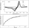 |
Fig. 5 Time evolution of the OH band difference spectrum for an ASW ice at 100 K. Top: the OH band shape changes as the ASW film restructures. Bottom: fitting the experimental date (dashed line) gives the reorganization timescale at 100 K. |
The difference spectrum time evolution is fitted with an Avrami equation. It was not possible to fit our data with an Avrami equation with a fixed n = 4 parameter. However, with a free n parameter (usually around 0.7), the rates obtained are similar, within a few percent, to the rates obtained using an exponential (Avrami equation with n = 1). The reorganization kinetic rates we measured are reported in Table 2, along with the Smith et al. (2011) crystallization rates at higher temperatures, between 140 K and 163 K.
Crystallization rates derived from the OH IR absorption band modification during the ASW crystallization process.
Smith et al. (2011) have deposited ASW films at a low temperature, 20 K, which are comparable to our 15 K deposited films. Our measured kinetic rates increase exponentially with the increasing temperature, as in Smith et al. (2011), with almost similar rates at 140 K. Our rate at 150 K, 9 × 10⁻⁴ s-1, is smaller than the value 1 × 10⁻² s-1 derived by Smith et al. (2011). However, Mate et al. (2012) reports a value closer to our value, 8.8 × 10⁻⁴ s-1, in ASW deposited at 14 K. If ASW is deposited at 120 K instead of 15 K, we find a reorganization rate of 7 × 10⁻³ s-1, which is closer to the Smith et al. (2011) value, 1 × 10⁻² s-1. The rate dependence with the deposition temperature we observe, is much larger than observed by Mate et al. (2012). This points out that the reorganization rate is dependent on the ice formation history. Figure 6 shows the temperature dependence of the ASW film reorganization rate and its dependence with the water vapor deposition temperature (inset in Fig. 6 ). This sensitivity to the ice formation history can induce dispersion on other physical properties such as diffusion.
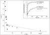 |
Fig. 6 Temperature dependance of the ASW reorganization rate for water vapor deposited at 15 K (crosses) and 120 K (square, at 150 K only) and fit with an Arrhenius law (dashed line). Our reorganization date are compared with Smith et al. (2011) crystallization values (circles). Inset: reorganization kinetics at 150 K for an ASW film made of water vapor deposited at 15 K and 120 K. |
For the same ASW film formation conditions, the reorganization rate follows an Arrhenius law. Figure 6 clearly shows the presence of two phenomena: the crystallization and a reorganization phenomenon at low temperature. Crystallization is the phase change between amorphous and crystalline ice and concerns the oxygen atom ordering that cannot take place at low-temperature because of the high activation energy required, 65.5 ± 0.5 kJ mol-1(Smith et al. 2011). We are not sure of the exact nature of the reorganization phenomenon we measure at low-temperature. It has an activation energy of 0.9 kJ mol-1, and could correspond to a proton ordering that occurs with a much lower activation energy than this for oxygen ordering. Jenniskens & Blake (1994) estimate the activation energy for the high- to low-density amorphous ice transition at less than 10 kJ mol-1, which corresponds to the change of coordination of the five-coordinated interstitial water. It may also be the transition between the low-density phase (Ial) and a third restrained amorphous phase (called Iar by Jenniskens & Blake 1994). This reorganization phenomenon could also correspond to a more mesoscopic crack reorganization or pore collapse (Manca et al. 2004), prior crystallization itself, through the motion of hydrogen bonds around their oxygen atoms, which corresponds to vacancy migration and disappearance prior crystallization. This mechanism manifests itself in the so-called molecular volcano phenomenon (Smith et al. 1997b).
This preliminary work on the ASW film reorganization points out that the ASW framework itself has reorganization kinetics that must be considered when dealing with the diffusion process.
3.1.2. The pore collapse
To characterize further the ASW film, we can address the issue of the thickness measurement more thoroughly. By growing an ice film at a high-vacuum pressure, we can compare the thickness derived from the interference technique and the thickness derived from the IR spectrum column density. The former measurement is linked to the optical thickness, while the latter measurement is related to the quantity of matter, which does not change with porosity. We assume that the compact ice density is ρ0 is 0.94 g/cm3, and we calculate the actual density ρ of the film from the optically determined thickness and the measured quantity of matter. We then calculate the porosity ν, defined as ν = 1 − ρ/ρ0.
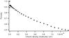 |
Fig. 7 Evolution of the porosity ν of the ASW ice during the deposition at 15 K. |
This experiment is performed at 15 K and we see in Fig. 7 that the porosity decreases globally as the film grows during deposition. This pore collapse has also been put in evidence by Bossa et al. (2012) while performing a temperature ramp on an porous ASW ice film. Therefore, we can assume that the first monolayers are very porous and fluffy, but during the deposition the porosity decreases and is stabilized to a lower value. For as long as we can record spectrum without saturating OH stretching bands, we do not reach the asymptotic value. We have not investigated whether the porosity evolution is a dynamic (time-dependent) relaxation process or if it is dependent on the amount of ice, nor have we investigated the temperature dependance of the porosity collapse. The pore collapse we measure looks higher than the value of 10% porosity collapse measured in Bossa et al. (2012) using a TPD experiment. This may be the difference between a temperature programmed desertion experiment and a deposition at a fixed temperature. Moreover, the porosity evolution is probably linked to the ASW relaxation. The isothermal porosity collapse should be investigated in future experiments. However, these experiment show that some error is induced in the evaluation of thickness d using a fixed density. An incorrect thickness estimation can lead to an error in the diffusion coefficient, and we think that the time evolution of porosity can be a significant cause of dispersion on the diffusion coefficients in porous ice.
3.2. Diffusion in porous amorphous ice
We deposit at 15 K a porous ASW ice film on top of a film of M molecules (M being CO, HNCO, HNCO, H2CO, or NH3), as it was described in Sect. 2. The ASW porosity can spread from microporosity to macroscopic cracks. It is not possible to evaluate the pore size distribution using FTIR spectroscopy only. The temperature of the ice layers is then promoted as quickly as possible (approximately 10 K/min) to a fixed temperature between 35 K and 140 K. The accessible range of temperature depends on the molecule. It is between 35 K and 40 K for CO, while it is between 110 K and 125 K for H2CO. At these fixed temperatures the M molecules diffuse in ASW before reaching the ASW surface and desorbing, as shown in Fig. 3 in the case of NH3. These isothermal experiments are repeated at different fixed temperatures in order to derive the temperature dependence of the diffusion coefficients.
To extract diffusion coefficients D (cm2 s-1) we will use Fick’s second law of diffusion, which corresponds to a thermal propagation of molecules in the ice. We will also use the Avrami equation to derive diffusion time constants. This equation is used to describes solid phase transitions at fixed temperature. It has been more particularly applied to describe the kinetics of crystallization (Smith et al. 2011). We have chosen this equation to compare time constants for diffusion and time constants for ice phase crystallization and reorganization in Sect. 3.4.
3.3. Analysis using Fick’s second law of diffusion
In order to model the IR decay curve [cm-2], we write down Fick’s second law of diffusion, for the M molecules density n(x,t) at a fixed temperature 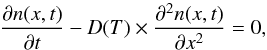 (4)where D(T) is the temperature dependent diffusion coefficient of the M molecules in the ASW film. Equation (4) is a propagation equation describing a one-dimensional diffusion of the M particles along the x direction.
The initial condition is taken as described in Sect. 2. The boundary conditions should reflect the absence of flux in the substrate at x = 0 and the instantaneous desorption at the surface of the ice layer x = d. Therefore, we set the boundary conditions to be dn(0,t)/dx = 0 and n(d,t) = 0, and the initial conditions to be n(x,0) = n0. With these initial and boundary conditions, using a series development (Crank 1975), we find a solution for Eq. (4) that gives the concentration profile of the density n(x,t) [cm-3] 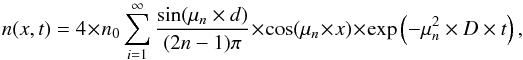 (5)where
  .
.
The time-dependent IR column density sFL(t) [cm-2] is calculated by numerically integrating n(x,t) from x = 0 to x = d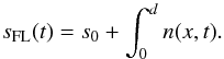 (6)The experimental IR decay curves are fitted to Eq. (6) to obtain the diffusion coefficients D(T) at the fixed temperature T, as shown in Fig. 3. In practice, the experimental curves do not reach zero, as expressed by the offset s0 in Eq. (6). One interpretation is to consider the remaining molecules to be trapped in the ASW film in closed pores (Collings et al. 2003). The typical amount of trapped molecules varies between 5 and 20% in our experimental conditions. Another interpretation is that these molecules do not participate in the surface diffusion process, but may diffuse much more slowy through the closed pores and the ASW volume, which corresponds to a bulk diffusion. This shows that a low-temperature ice deposition, 15 K here, favors a c.a 90% surface diffusion and a c.a 10% bulk diffusion or trapping. The uncertainty on the fit results is approximately 10%. We estimate a dispersion of approximately 90% on the measured diffusion coefficients from five measurements performed on NH3 at 117 K.
The isothermal diffusion experiments are repeated at several temperatures for the different M molecules and the diffusion coefficients derived from fitting the experimental data with Fick’s second law of diffusion are summarized in Table 3, along with measured thicknesses both in nm and in units of ML. These diffusion coefficient are consistent with those found by Livingston et al. (2002).
We see in Fig. 3, however, that the adequacy between the theoretical curve and the experimental curve is not good. This poor adequacy is doubled by a high dispersion on the measured diffusion coefficients. There may be several reasons for this poor agreement. On reason would be that there is a distribution of diffusion coefficients (corresponding to a distribution of sizes of cracks and pores) and not a single diffusion coefficient. Convoluting the diffusion coefficient with a distribution of pores on the basis of Mispelaer et al. (2012) improves the adequacy between the theoretical and experimental curve, but will add one more parameter to fit, the shape factor of the distribution. But this does not necessarily give more physical insight into the diffusion problem. This kind of refinement is useless given the large uncertainty we have on the diffusion coefficients. Another reason for the poor adequacy would be that since the measured diffusion is a surface diffusion alongs cracks and pores, the diffusion length is not the macroscopic ASW film thickness d, but a distribution of diffusion lengths, according to the meanders of the different cracks and pores, the effective diffusion thickness being longer. Another reason, that will be discussed in Sect. 3.1, is because the thickness is not constant with time, but shrinks as the ASW film is reorganizing and crystallizing. However, fitting the experimental data with a one-dimensional propagation equation and a single diffusion coefficient gives satisfactory enough diffusion coefficients. Going beyond this simple mathematical treatment will add more parameters that we would not be able to extract from our measurements.
Experimental diffusion rates D (cm2 s-1) for CO, HNCO, H2CO, and NH3 in ASW as a function of temperature, derived from either Fick’s second law of diffusion or from an Avrami equation.
3.4. Analysis using an Avrami equation
In a second approach, the IR decay curves are fitted against an Avrami equation. The Avrami equation can account for long-range diffusion-limited growth, or in our case, it can account for how fast the solid-state molecules M(s) are diffusing to the surface to transform into gas-phase molecules M(g). Moreover, this equation has the advantage of directly giving a time constant in s-1 for the diffusion of the molecules crossing an ASW ice mantle of thickness d, which is a useful parameter since it can be compared to other rates such as the amorphous-to-crystalline phase change rate. We first try to fix n = 4 in Eq. (3) and derive kAv by fitting experimental isothermal IR decay curves as shown in Fig. 3. With n = 4, there is no agreement between experimental and theoretical curves so we leave n as a free parameter as well.
The resulting values for kAv and n are summarized in Table 4. We see that the best fits are obtained with an n parameter around 0.7 in all cases. We also see in Fig. 3 that the agreement between the experimental data and the theoretical curve calculated using the Avrami equation is much better.
Diffusion rates kAv (s-1) and order n for CO, HNCO, H2CO, and NH3 derived using an Avrami equation.
For the sake of comparison with diffusion coefficients derived from the Fick diffusion law, we can give the order of magnitude for the diffusion coefficients (in cm2 s-1) using the rate constant (in s-1) in Table 4 derived from the Avrami equation using the approximate relation (Livingston et al. 2002) 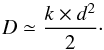 (7)The derived values for kAv are transformed into a diffusion coefficient using Eq. (7) and are summarized in Table 3. We can see the rather good agreement between the two diffusion coefficients, given the approximation done in Eq. (7). The uncertainties on the diffusion coefficient derived from kAv (about 10% uncertainty) are not reported since the uncertainty on the thickness d is hard to define, as explained in Sect. 3.1.2.
3.5. Temperature dependence of the diffusion coefficients
From the diffusion coefficients measured at several temperatures and summarized in Table 3, we obtain the temperature dependence of the diffusion rate D(T) for the different molecules, as shown in Fig. 8.
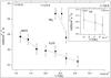 |
Fig. 8 Logarithm of the diffusion coefficient as a function of the inverse of the temperature for HNCO (squares), H2CO (circles), and NH3 (triangles) and for CO (crosses, in the inset), as obtained from the diffusion equation. The errors bars are evaluated from dispersion measurements on NH3 at 117 K, and are probably overestimated for CO. The temperature dependence of the diffusion coefficients is fitted against an Arrhenius equation (solid lines). |
Fitting the experimental diffusion rates measured at different temperatures with an Arrhenius law 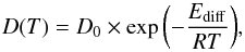 (8)where Ediff (kJ mol-1) is the activation energy for diffusion, and D0 the diffusion pre-exponential factor. Because of the 90% uncertainty on each diffusion coefficient value and to the limited temperature range inherent to our experimental protocol, the uncertainties on both Ediff and ν0 are high, and the two parameters are highly correlated. The large, correlated uncertainties prevent us from a confident extrapolation to lower temperatures, which would be more relevant to astrochemistry. The activation energy for diffusion for CO, 1.0 ± 1.5 kJ mol-1, is in agreement with the value calculated by Karssemeijer et al. (2012), 50 ± 1 meV or 4.8 ± 1 kJ mol-1, or with a fraction to the value measured and calculated for CO-ice interaction (Manca et al. 2001). The activation energy for diffusion of 12 ± 2 kJ mol-1 for H2CO is on the order of the magnitude of the energy required to break a hydrogen bond (≃10 kJ mol-1). The activation energies found for HNCO (25 ± 7 kJ mol-1) and NH3 (66 ± 48 kJ mol-1) are higher. This is because of the larger dipole moment of a NH bond compared to a CH bond, making HNCO and NH3 more bounded to the H2O network than H2CO. We notice that comparing the values at 115 K and 120 K for H2CO and NH3 for the diffusion coefficients that they do not scale as the square root of the mass, indicating that the mass of the molecule is not the dominant parameter.
3.6. Influence of the ASW crystallization on the diffusion
The poor adequacy between the experimental curves and the theoretical curves obtained from the diffusion equation and the large dispersion on the diffusion coefficients should be investigated further. Moreover, the good adequacy of our diffusion induced IR decay curves with an Avrami equation, which is usually used to study phase changes, raises the question of the physical origin of the diffusion. In order to test the possible relationship between diffusion and crystallization phase changes (Jenniskens & Blake 1994; Jenniskens et al. 1995; Hodyss et al. 2008; Öberg et al. 2009), we can compare the measured diffusion rates (in s-1) for the different molecules, as obtained using the Avrami equation, to the ASW ice crystallization and reorganization rates investigated in Sect. 3.1.1, as shown in Fig. 9. Because of the sensitivity of this rate to the experimental conditions, it is important to compare reorganization and diffusion rates derived from the same experiment. The sensitivity to the ice formation history may explain the large dispersion interval our measured diffusion coefficients exhibit.
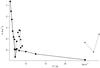 |
Fig. 9 Comparison of the crystallization rate (diamonds with solid lines) and of the diffusion rate as a function of temperature for CO (crosses), HNCO (squares), H2CO (circles), and NH3 (triangles). |
Figure 9 shows that the CO diffusion is much faster than the reorganization rate for the 35–40 K interval, and its diffusion should be decorrelated from the reorganization process, although they have similar activation energies. The pore collapse associated to ASW reorganization implies the formation of hydrogen bonds and an increase in coordination of the H2O molecules, which can be on the same order as the CO-H2O bonds.
The measured diffusion rates for the hydrogen bonded molecules, H2CO, HNCO, and NH3, have orders of magnitude similar to the ASW crystallization rate. The diffusion and ASW crystallization timescales similarity may be coincidental, based on energetic arguments only. Indeed, surface diffusion on the ice surface involves physisorption energies that are related to the breaking and forming of hydrogen bonds withe H2O molecules, while the adsorbate is diffusing on the surface. Rearranging H2O molecules from an amorphous ice to a crystalline ice also involves the formation and destruction of hydrogen bonds, which may explain why diffusion and crystallization rates have the same order of magnitude. Moreover, the hydrogen bonded species probably exist as hydrates in the ice and thus behave like H2O molecules, following them in their rearrangement. This argument is strengthened by the fact that the diffusion activation energies for H2CO, HNCO, and NH3 are increasing with the strength of the hydrogen bonding. The H2CO molecule has two weakly polar CH donor hydrogen bonds, while HNCO and NH3 have one and three donor hydrogen bonds, respectively. One can, alternatively, think the whole ASW grid is restructuring and that the M molecules settling on the grid points are swept away when the whole H2O network is restructuring. The mathematical treatment of particles diffusing in a moving grid is complex (Sinai 1982) and beyond the scope of this work.
Although it is not possible to conclude whether or not both rates are linked by a causality relationship on the basis of orders of magnitude of timescales only, one can suspect that the crystallization has an influence on hydrogen bonded molecules surface diffusion. The metastable ASW rearrangement and crystallization concomitant phenomena may be at least a source of a large spread on the measured surface diffusion coefficients.
This rearrangement phenomenon can be related to the self-diffusivity of ASW as discussed in Livingston et al. (2002) and Smith (2000), and to the swapping mechanism developed by Öberg et al. (2009) and Fayolle et al. (2011). We can consider that a restructuring amorphous solid has a diffusivity of vacancies toward the formation of a vacancy-free crystal. There is evidence for a vacancy-controlled diffusion mechanism for molecules in ices (Goto et al. 1986; Hondoh et al. 1989; Livingston et al. 2002) at T ≤ 223 K. The similarity between the diffusion coefficients of hydrogen bonded molecules and their correlation with the crystallization curve could be explained by a self-diffusivity of H2O molecules during the phase change, producing a displacement of vacancies, which induces a displacement of the host-molecule; this is the so-called Schottky mechanism. The difference in vacancy density from one ice deposition to another could be a source of dispersion in our experiments. This ASW crystallization induced diffusion is due to the rearrangement of the ASW framework, and is different in nature from the thermal diffusion of the M molecules from one physisorption site to another.
Of course both the thermal diffusion and the ASW phase change diffusion can coexist and both can contribute to the overall diffusion. The relationship between the ASW phase change and the diffusion of the host molecules is hard to disentangle and needs to be investigated more thoroughly. This crystallization driven diffusion would be of prime importance if a continuous mechanism of amorphization exists, such as VUV photons (Kouchi & Kuroda 1990), that counterbalances a continuous crystallization mechanism. This would induce a continuous diffusion of the reactants in the ice mantle and would lead to an enhanced grain chemistry.
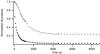 |
Fig. 10 Time evolution of the abundance of NH3 (squares) and H2O (circles) in a compact ASW ice at 130 K. The ASW ice has been deposited on top of the NH3 film. NH3 and H2O are monitored on their characteristic absorption bands at 1100 cm-1 and 1660 cm-1, respectively. Both time evolutions have similar decay rates, indicating that the NH3 molecules are co-desorbing with the ASW ice. |
Although very difficult to perform in a measurable and reproducible way in laboratory, it is important to study the variation in pores and vacancy densities. Depositing the ASW ice from a low-temperature H2O vapor and not from room temperature water vapor would enable us to get a hint on whether the measured diffusion coefficients are fully astrophysically relevant and as such if they can be applied to a gas-grain model or if there is part of the experimental artifact due to the out-of-equilibrium state of laboratory produced ice analogues. These questions are far from trivial to answer and need a large amount of work. Thus, it would be interesting to compare experimental results obtained from different experimental procedures and experimental set-ups from different laboratories, to estimate the spread between different ice analogues.
3.7. Diffusion in compact amorphous ice
We deposit a first 10 nm thick layer of a M molecules (M being CO, HNCO, HNCO, H2CO, or NH3) at 15 K. Then the temperature is set to 100 K and a 100 nm thick layer of H2O is deposited on top of it at 100 K. The deposited water ice structure is thus amorphous and compact, as the interstellar ice is thought to be (Keane et al. 2001). This precludes the formation of a pore network and the possibility of having surface diffusion in the ASW ice along pores and cracks. The only way for the molecules to reach the surface is to diffuse within the bulk of ASW. The ASW layer thickness is estimated using the H2O bending mode IR absorption bands. It is not possible to apply this experimental protocol to CO since it is desorbing when T is greater than 40 K. The temperature of the ice layers is then promoted as fas as possible to a fixed temperature between 100 K and 140 K. The characteristic IR absorption bands of the M molecules are monitored along with time at this fixed temperature. Unlike the diffusion in porous ASW where surface diffusion is favored, we are not able to observe the IR bands decreasing as they were in Fig. 3. First the molecular bands get thinner, which indicates the M molecular solid is crystallizing. Second, the M species IR bands are decreasing, but this decrease is correlated to the ASW IR bands decrease, as shown in Fig. 10 for NH3. This means that for an approximately 100 monolayer thick ice mantle, which is an upper limit for the interstellar ice mantle thickness, the desorption of the H2O mantle is faster than the diffusion of other molecules through the mantle. Most of the molecules present in the mantle will co-desorb along with the mantle (Collings et al. 2004) before reaching the surface and desorbing. Thus, an upper limit to the diffusion coefficients can be set at 10-15 cm2 s-1 for temperatures between 100 K and 140 K. An order of magnitude for bulk diffusion on amorphous ASW was estimated by Smith et al. (1997a) at 10−12±1 cm2 s-1 at 155 K. Low diffusion coefficients prevent the occurrence of a diffusion-limited chemistry, i.e., other than statistical, in the bulk of the mantle. However, during the ice mantle desorption a significant amount of the host molecules are diffusing and co-desorbing, which could induce chemical reactions during the desorption time interval. Further studies are needed on thinner ASW films since a diffusion of a few monolayers is needed to be astrochemically relevant.
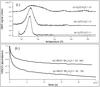 |
Fig. 11 i.) A temperature programmed desorption experiment in a H2CO:H2O ice mixture in a (a) 1:1, (b) 1:3, (c) 1:10 concentration ratio showing the desorption of surface H2CO feature (M), along with the volcano desorption feature (V) and the co-desorption with H2O feature (C) (from Noble et al. 2012). The M desorption feature of H2CO is affected by the need for H2CO to diffuse upward to the surface before desorbing. ii.) The isothermal kinetics of the HNCO + NH3 → OCN− + NH |

4. Astrophysical implications
The diffusion process is of prime importance in solid-state astrochemistry. First, it is coupled to molecular desorption when the ice thickness is greater then one monolayer on the interstellar grains. As shown in Fig. 11(i.), the desorption of H2CO within multilayer ice is slowed down, because the H2CO mantle molecule needs to first diffuse to the upper monolayer (the surface) in order to desorb (Noble et al. 2012). The H2CO desorption feature is therefore broadened and shifted to higher temperatures, since diffusion delays the H2CO. Second, diffusion limits reactivity when reactants are diluted into water ice. As shown in Fig. 11(ii.), the time decay curve of the HNCO reactant is affected by its dilution into ASW ice in the HNCO + NH3 reaction (Mispelaer et al. 2012). Diffusion-limited desorption and diffusion-limited reactivity dominate ASW ice chemistry and their quantitative understanding depends on diffusion coefficient measurements such as those presented in this paper. Accounting for the diffusion limitation in gas-grain models is highly important for reproducing volatile complex molecules in hot cores and hot corinos.
The bulk diffusion coefficient is related to the delayed desorption shown in Fig. 11(i.) and to the mantle to surface transition in three-phase gas-grain models (Hasegawa & Herbst 1993). Applying Eq. (7) with the 10-15 cm2 s-1 upper limit we have estimated for the bulk diffusion coefficient and a 100 nm mantle thickness, we have a timescale for mantle to surface transition that is 15 years lower. Contrary to the derivation made in (Hasegawa & Herbst 1993), the bulk to surface transition rate is molecule dependent, and does not depend statistically on the fraction of each mantle species over the total number of mantle molecules. The surface diffusion coefficient is related to the surface diffusion rate Rdiff (i.e., the frequency of sweeping the surface area of an average grain) that determines the surface reaction rate in the diffusion-limited case expressed in Eq. (5) in Hasegawa et al. (1992).
The possible correlation between species diffusion in ice and ASW ice crystallization also has implications in astrochemistry and in the formation of complex organic molecules. In both purely thermal reactions and photochemical reactions, either electronically stable molecules or radicals need to diffuse on top of an ice surface or within the ice bulk to meet and react together. Their diffusion is limited by their mass and by their surface binding energy. This puts constraints on their mobility, on the formation of complex molecules, and also enables a certain chemical selectivity since the more mobile molecules will react more easily. If ASW ice crystallization drives the diffusion process, this will enable the diffusion of even weakly mobile molecules and then will enhance the ice reactivity and the formation of complex organic molecules. This crystallization driven diffusion would be of prime importance if a continuous mechanism of amorphization existed, such as VUV photons (Kouchi & Kuroda 1990) that counterbalance a continuous crystallization mechanism, as this would induces a continuous diffusion of the reactants in the ice mantle. Of course, both the thermal diffusion and the ASW phase change diffusion can coexist and both can contribute to the overall diffusion. The relationship between the ASW phase change and the diffusion of the host molecules is hard to disentangle and needs to be investigated more thoroughly, because of its importance in ice chemistry and n the formation of complex organic molecules.
The lack of knowledge in the morphology of interstellar ice is an issue when dealing with diffusion. First the porosity, i.e., the ratio between effective surface and bulk, is poorly known and so is the part of surface diffusion versus bulk diffusion. Second, diffusion in amorphous ice is different from diffusion in between grain boundaries in polycrystalline ice. Thus, it is important to understand the diffusion mechanisms and to couple these diffusion studies to structural studies on interstellar ice analogues. The correspondence between interstellar ice and its laboratory analogues must be considered carefully.
Another issue is that interstellar ice is not only made of water. The other constituents (such as CO2, CO, etc) can affect the diffusion coefficient of a species and the porosity of the ice. Such mixtures must be considered at a later time.
5. Conclusion
We have measured the surface diffusion coefficients of CO, HNCO, H2CO, and NH3 in ASW at low-temperature using FTIR spectroscopy.
In compact ASW ice, where bulk diffusion is favored, we can only set an upper limit of 10-15 cm2 s-1 for the bulk diffusion coefficients for temperatures ranging between 100 K and 130 K. Bulk diffusion within thick ice is slower than ASW desorption for HNCO, H2CO, and NH3. Bulk diffusion on thinner ice is more relevant to solid-state chemistry and should be investigated further.
In porous ASW ice, where the effective surface is favored through cracks and pores, we can observe a surface diffusion of molecules on the ice surface and model it by Fick’s second law of diffusion. The diffusion coefficients have been measured to be between 10-11 and 10-14 cm2 s-1 for temperatures ranging between 35 K and 135 K depending on the molecule, as summarized in Table 3. Because of the limited temperature range of our experiment and because of the large spread on each measurement, it is difficult to derive accurate diffusion energies.
This study shows that a surface chemistry involving heavy species is therefore possible on amorphous ice surface, and gives an order of magnitude for their diffusion coefficients. The diffusion activation energy for weakly hydrogen bonded CO is about one kJ mol-1, while it is of a few tens of kJ mol-1 for hydrogen bonded molecules (H2CO, HNCO, and NH3), increasing as the hydrogen bonding strength between the molecules and the ASW ice increases. This corresponds to the energy range of physisorbed hydrogen bonded molecules thermally diffusing on the ice surface.
We have also put into evidence the ASW film reorganization on laboratory ice analogues between 40 K and 130 K. It is not clear whether or not this low-temperature reorganization and the ASW crystallization occurring above 130 K affect the diffusion of the species in the ice, but this possibility should definitely be considered.
Acknowledgments
This work has been funded by the French national programme Physique Chimie du Milieu Interstellaire (PCMI) and the Centre National d’Études Spatiales (CNES). P.T and T.H. would like to thank the ORCHID France-Taiwan exchange program. The authors would like to thank the referees for the time they spent in improving this manuscript.
References
- Accolla, M., Congiu, E., Dulieu, F., et al. 2011, Phys. Chem. Chem. Phys., 13, 8037 [NASA ADS] [CrossRef] [Google Scholar]
- Avrami, M. 1939, J. Chem. Phys., 7, 1103 [NASA ADS] [CrossRef] [Google Scholar]
- Avrami, M. 1940, J. Chem. Phys., 8, 212 [Google Scholar]
- Avrami, M. 1941, J. Chem. Phys., 9, 177 [NASA ADS] [CrossRef] [Google Scholar]
- Baragiola, R. A., Burke, D. J., & Fama, M. A. 2009, AGU Fall Meeting Abstracts [Google Scholar]
- Boogert, A. C. A., Pontoppidan, K. M., Lahuis, F., et al. 2004, ApJS, 154, 359 [NASA ADS] [CrossRef] [Google Scholar]
- Boogert, A. C. A., Pontoppidan, K. M., Knez, C., et al. 2008, ApJ, 678, 985 [NASA ADS] [CrossRef] [Google Scholar]
- Bossa, J. B., Theulé, P., Duvernay, F., & Chiavassa, T. 2009, ApJ, 707, 1524 [NASA ADS] [CrossRef] [Google Scholar]
- Bossa, J.-B., Isokoski, K., de Valois, M. S., & Linnartz, H. 2012, A&A, 545, A82 [NASA ADS] [CrossRef] [EDP Sciences] [Google Scholar]
- Collings, M. P., Dever, J. W., Fraser, H. J., McCoustra, M. R. S., & Williams, D. A. 2003, ApJ, 583, 1058 [NASA ADS] [CrossRef] [Google Scholar]
- Collings, M. P., Anderson, M. A., Chen, R., et al. 2004, MNRAS, 354, 1133 [NASA ADS] [CrossRef] [Google Scholar]
- Crank, J. 1975, The Mathematics of Diffusion (Oxford: Clarendon Press), UK [Google Scholar]
- Dartois, E. 2005, Space Sci. Rev., 119, 293 [NASA ADS] [CrossRef] [Google Scholar]
- Demyk, K., Dartois, E., D’Hendecourt, L., et al. 1998, A&A, 339, 553 [NASA ADS] [Google Scholar]
- Fayolle, E. C., Öberg, K. I., Cuppen, H. M., Visser, R., & Linnartz, H. 2011, A&A, 529, A74 [NASA ADS] [CrossRef] [EDP Sciences] [Google Scholar]
- Garrod, R. T., Weaver, S. L. W., & Herbst, E. 2008, ApJ, 682, 283 [NASA ADS] [CrossRef] [Google Scholar]
- Gerakines, P. A., Schutte, W. A., Greenberg, J. M., & van Dishoeck, E. F. 1995, A&A, 296, 810 [NASA ADS] [Google Scholar]
- Gibb, E. L., Whittet, D. C. B., Boogert, A. C. A., & Tielens, A. G. G. M. 2004, ApJS, 151, 35 [NASA ADS] [CrossRef] [PubMed] [Google Scholar]
- Goto, K., Hondoh, T., & Higashi, A. 1986, Japanese J. Appl. Phys., 25, 351 [NASA ADS] [CrossRef] [Google Scholar]
- Hasegawa, T. I., & Herbst, E. 1993, MNRAS, 263, 589 [NASA ADS] [CrossRef] [Google Scholar]
- Hasegawa, T. I., Herbst, E., & Leung, C. M. 1992, ApJS, 82, 167 [NASA ADS] [CrossRef] [Google Scholar]
- Hodyss, R., Johnson, P. V., Orzechowska, G. E., Goguen, J. D., & Kanik, I. 2008, Icarus, 194, 836 [NASA ADS] [CrossRef] [Google Scholar]
- Hondoh, T., Goto, A., Hoshi, R., et al. 1989, Rev. Sci. Instr., 60, 2494 [NASA ADS] [CrossRef] [Google Scholar]
- Jenniskens, P., & Blake, D. F. 1994, Science, 265, 753 [NASA ADS] [CrossRef] [Google Scholar]
- Jenniskens, P., Blake, D. F., Wilson, M. A., & Pohorille, A. 1995, ApJ, 455, 389 [NASA ADS] [CrossRef] [Google Scholar]
- Karssemeijer, L. J., Pedersen, A., Jonsson, H., & Cuppen, H. 2012, Phys. Chem. Chem. Phys., accepted [Google Scholar]
- Keane, J. V., Boogert, A. C. A., Tielens, A. G. G. M., Ehrenfreund, P., & Schutte, W. A. 2001, A&A, 375, L43 [NASA ADS] [CrossRef] [EDP Sciences] [Google Scholar]
- Kerkhof, O., Schutte, W. A., & Ehrenfreund, P. 1999, A&A, 346, 990 [NASA ADS] [Google Scholar]
- Knez, C., Boogert, A. C. A., Pontoppidan, K. M., et al. 2005, ApJ, 635, L145 [NASA ADS] [CrossRef] [Google Scholar]
- Kouchi, A., & Kuroda, T. 1990, Nature, 344, 134 [NASA ADS] [CrossRef] [Google Scholar]
- Lattelais, M., Bertin, M., Mokrane, H., et al. 2011, A&A, 532, A12 [NASA ADS] [CrossRef] [EDP Sciences] [Google Scholar]
- Livingston, F. E., Smith, J. A., & George, S. M. 2002, J. Phys. Chem. A, 106, 6309 [CrossRef] [Google Scholar]
- Manca, C., Martin, C., Allouche, A., & Roubin, P. 2001, J. Phys. Chem. B, 51, 12861 [CrossRef] [Google Scholar]
- Manca, C., Martin, C., & Roubin, P. 2002, Chem. Phys. Lett., 364, 220 [NASA ADS] [CrossRef] [Google Scholar]
- Manca, C., Martin, C., & Roubin, P. 2004, Chem. Phys. Lett., 300, 53 [Google Scholar]
- Mate, B., Rodriguez-Lazcano, Y., & Herrero, V. J. 2012, Phys. Chem. Chem. Phys., accepted [Google Scholar]
- Mayer, E., & Pletzer, R. 1986, Nature, 319, 298 [NASA ADS] [CrossRef] [Google Scholar]
- Mispelaer, F., Theulé, P., Duvernay, F., Roubin, P., & Chiavassa, T. 2012, A&A, 540, A40 [NASA ADS] [CrossRef] [EDP Sciences] [Google Scholar]
- Noble, J., Theulé, P., Mispelaer, F., et al. 2012, A&A, 543, A5 [NASA ADS] [CrossRef] [EDP Sciences] [Google Scholar]
- Öberg, K. I., Fayolle, E. C., Cuppen, H. M., van Dishoeck, E. F., & Linnartz, H. 2009, A&A, 505, 183 [NASA ADS] [CrossRef] [EDP Sciences] [Google Scholar]
- Palumbo, M. E. 2006, A&A, 453, 903 [NASA ADS] [CrossRef] [EDP Sciences] [MathSciNet] [Google Scholar]
- Palumbo, M. E., Baratta, G. A., Leto, G., & Strazzulla, G. 2010, J. Mol. Struct., 972, 64 [NASA ADS] [CrossRef] [Google Scholar]
- Raut, U., Famá, M., Loeffler, M. J., & Baragiola, R. A. 2008, ApJ, 687, 1070 [NASA ADS] [CrossRef] [Google Scholar]
- Redhead, P. A. 1962, Vacuum, 12, 203 [CrossRef] [Google Scholar]
- Rowland, B., Fisher, M., & Devlin, J. P. 1991, J. Chem. Phys., 95, 1378 [NASA ADS] [CrossRef] [Google Scholar]
- Schutte, W. A., Gerakines, P. A., Geballe, T. R., van Dishoeck, E. F., & Greenberg, J. M. 1996, A&A, 309, 633 [NASA ADS] [Google Scholar]
- Smith, R. 2000, Chem. Phys., 258, 291 [NASA ADS] [CrossRef] [Google Scholar]
- Smith, R. S., Huang, C., & Kay, B. D. 1997a, J. Phys. Chem. B, 101, 6123 [CrossRef] [Google Scholar]
- Smith, R. S., Huang, C., Wong, E. K. L., & Kay, B. D. 1997b, Phys. Rev. Lett., 79, 909 [NASA ADS] [CrossRef] [Google Scholar]
- Smith, R. S., Matthiesen, J., & Kay, B. D. 2010, J. Chem. Phys., 133, 174504 [NASA ADS] [CrossRef] [Google Scholar]
- Smith, R. S., Matthiesen, J., Knox, J., & Kay, B. D. 2011, J. Phys. Chem. A, 115, 5908 [CrossRef] [Google Scholar]
- Tielens, A. G. G. M., & Allamandola, L. J. 1987, Interstellar Processes, 134, 397 [NASA ADS] [CrossRef] [Google Scholar]
- Theulé, P., Duvernay, F., Ilmane, A., et al. 2011, A&A, 530, A96 [NASA ADS] [CrossRef] [EDP Sciences] [Google Scholar]
- van Broekhuizen, F. A., Keane, J. V., & Schutte, W. A. 2004, A&A, 415, 425 [NASA ADS] [CrossRef] [EDP Sciences] [Google Scholar]
- Watanabe, N., & Kouchi, A. 2002, ApJ, 571, L173 [NASA ADS] [CrossRef] [Google Scholar]
- Whittet, D. C. B., Bode, M. F., Baines, D. W. T., Longmore, A. J., & Evans, A. 1983, Nature, 303, 218 [NASA ADS] [CrossRef] [Google Scholar]
- Ya, G. S. 1982, Theory Prob. Appl., 27, 256 [Google Scholar]
- Zondlo, M. A., Onasch, T. B., Warshawsky, M. S., et al. 1997, J. Phys. Chem. B, 101, 10887 [CrossRef] [Google Scholar]
All Tables
Frequency positions and integrated band strengths of solid-state molecules at 10 K.
Crystallization rates derived from the OH IR absorption band modification during the ASW crystallization process.
Experimental diffusion rates D (cm2 s-1) for CO, HNCO, H2CO, and NH3 in ASW as a function of temperature, derived from either Fick’s second law of diffusion or from an Avrami equation.
Diffusion rates kAv (s-1) and order n for CO, HNCO, H2CO, and NH3 derived using an Avrami equation.
All Figures
|
Fig. 1 Scheme of the bilayer sample: a thin layer of the studied M molecule (M being CO, HNCO, H2CO, or NH3) is first deposited at 15 K on the gold surface, and then a thicker layer of ASW ice is deposited on top of it at 15 K. The thickness d of the ASW layer is estimated both using H2O IR absorption bands and by interferometry. The diffusion of the M molecule along the x direction is monitored at a fixed temperature by recording the evolution of one of its characteristic IR absorption bands as function of time using FTIR spectroscopy. A compact ASW ice favors a bulk (volume) diffusion (left part), while a porous ASW ice favors a surface diffusion along cracks and pores (surface). |
| In the text | |
|
Fig. 2 Infrared spectrum of a NH3:ASW bilayer film at 15 K. The quantity of deposited NH3 and H2O are derived from their characteristic absorption bands. The diffusion of NH3 along the x direction at a fixed temperature T will be monitored by recording the decay of its characteristic absorption band at 1110 cm-1 as a function of time. |
| In the text | |
|
Fig. 3 Isothermal diffusion of NH3 through a porous ASW layer at 115 K. Markers: experimental IR decay curve sexp(t) of NH3. Theoretical curve sfl(t) using the Fick’s second law for diffusion (dashed line). Theoretical curve sfl(t) using the Avrami equation (solid line). |
| In the text | |
|
Fig. 4 He-Ne laser interference fringes pattern obtained during the ASW film deposition at 15 K. |
| In the text | |
|
Fig. 5 Time evolution of the OH band difference spectrum for an ASW ice at 100 K. Top: the OH band shape changes as the ASW film restructures. Bottom: fitting the experimental date (dashed line) gives the reorganization timescale at 100 K. |
| In the text | |
|
Fig. 6 Temperature dependance of the ASW reorganization rate for water vapor deposited at 15 K (crosses) and 120 K (square, at 150 K only) and fit with an Arrhenius law (dashed line). Our reorganization date are compared with Smith et al. (2011) crystallization values (circles). Inset: reorganization kinetics at 150 K for an ASW film made of water vapor deposited at 15 K and 120 K. |
| In the text | |
|
Fig. 7 Evolution of the porosity ν of the ASW ice during the deposition at 15 K. |
| In the text | |
|
Fig. 8 Logarithm of the diffusion coefficient as a function of the inverse of the temperature for HNCO (squares), H2CO (circles), and NH3 (triangles) and for CO (crosses, in the inset), as obtained from the diffusion equation. The errors bars are evaluated from dispersion measurements on NH3 at 117 K, and are probably overestimated for CO. The temperature dependence of the diffusion coefficients is fitted against an Arrhenius equation (solid lines). |
| In the text | |
|
Fig. 9 Comparison of the crystallization rate (diamonds with solid lines) and of the diffusion rate as a function of temperature for CO (crosses), HNCO (squares), H2CO (circles), and NH3 (triangles). |
| In the text | |
|
Fig. 10 Time evolution of the abundance of NH3 (squares) and H2O (circles) in a compact ASW ice at 130 K. The ASW ice has been deposited on top of the NH3 film. NH3 and H2O are monitored on their characteristic absorption bands at 1100 cm-1 and 1660 cm-1, respectively. Both time evolutions have similar decay rates, indicating that the NH3 molecules are co-desorbing with the ASW ice. |
| In the text | |
|
Fig. 11 i.) A temperature programmed desorption experiment in a H2CO:H2O ice mixture in a (a) 1:1, (b) 1:3, (c) 1:10 concentration ratio showing the desorption of surface H2CO feature (M), along with the volcano desorption feature (V) and the co-desorption with H2O feature (C) (from Noble et al. 2012). The M desorption feature of H2CO is affected by the need for H2CO to diffuse upward to the surface before desorbing. ii.) The isothermal kinetics of the HNCO + NH3 → OCN− + NH |
| In the text | |
Current usage metrics show cumulative count of Article Views (full-text article views including HTML views, PDF and ePub downloads, according to the available data) and Abstracts Views on Vision4Press platform.
Data correspond to usage on the plateform after 2015. The current usage metrics is available 48-96 hours after online publication and is updated daily on week days.
Initial download of the metrics may take a while.