| Issue |
A&A
Volume 554, June 2013
|
|
|---|---|---|
| Article Number | A112 | |
| Number of page(s) | 9 | |
| Section | Numerical methods and codes | |
| DOI | https://doi.org/10.1051/0004-6361/201321494 | |
| Published online | 14 June 2013 | |
Libsharp – spherical harmonic transforms revisited
1 Max-Planck-Institut für Astrophysik, Karl-Schwarzschild-Str. 1, 85741 Garching, Germany
e-mail: This email address is being protected from spambots. You need JavaScript enabled to view it.
2 Institute of Theoretical Astrophysics, University of Oslo, PO Box 1029 Blindern, 0315 Oslo, Norway
e-mail: This email address is being protected from spambots. You need JavaScript enabled to view it.
Received: 18 March 2013
Accepted: 14 April 2013
Abstract
We present libsharp, a code library for spherical harmonic transforms (SHTs), which evolved from the libpsht library and addresses several of its shortcomings, such as adding MPI support for distributed memory systems and SHTs of fields with arbitrary spin, but also supporting new developments in CPU instruction sets like the Advanced Vector Extensions (AVX) or fused multiply-accumulate (FMA) instructions. The library is implemented in portable C99 and provides an interface that can be easily accessed from other programming languages such as C++, Fortran, Python, etc. Generally, libsharp’s performance is at least on par with that of its predecessor; however, significant improvements were made to the algorithms for scalar SHTs, which are roughly twice as fast when using the same CPU capabilities. The library is available at http://sourceforge.net/projects/libsharp/ under the terms of the GNU General Public License.
Key words: methods: numerical / cosmic background radiation / large-scale structure of Universe
© ESO, 2013
1. Motivation
While the original libpsht library presented by Reinecke (2011) fulfilled most requirements on an implementation of spherical harmonic transforms (SHTs) in the astrophysical context at the time, it still left several points unaddressed. Some of those were already mentioned in the original publication: support for SHTs of arbitrary spins and parallelisation on computers with distributed memory.
Both of these features have been added to libpsht in the meantime, but other, more technical, shortcomings of the library have become obvious since its publication, which could not be fixed within the libpsht framework.
One of these complications is that the library design did not anticipate the rapid evolution of microprocessors during the past few years. While the code supports both traditional scalar arithmetic as well as SSE2 instructions, adding support for the newly released Advanced Vector Extensions (AVX) and fused multiply-accumulate instructions (FMA3/FMA4) would require adding significant amounts of new code to the library, which is inconvenient and very likely to become a maintenance burden in the long run. Using proper abstraction techniques, adding a new set of CPU instructions could be achieved by only very small changes to the code, but the need for this was unfortunately not anticipated when libpsht was written.
Also, several new, highly efficient SHT implementations have been published in the meantime; most notably Wavemoth (Seljebotn 2012) and shtns (Schaeffer 2013). These codes demonstrate that libpsht’s computational core did not make the best possible use of the available CPU resources. Note that Wavemoth is currently an experimental research code not meant for general use.
To address both of these concerns, the library was redesigned from scratch. The internal changes also led to a small loss of functionality; the new code no longer supports multiple simultaneous SHTs of different type (i.e. having different directions or different spins). Simultaneous transforms of identical type are still available, however.
As a fortunate consequence of this slight reduction in functionality, the user interface could be simplified dramatically, which is especially helpful when interfacing the library with other programming languages.
Since backward compatibility is lost, the new name libsharp was chosen for the resulting code, as a shorthand for “Spherical HARmonic Package”.
The decision to develop libsharp instead of simply using shtns was taken for various reasons: shtns does not support spin SHTs or allow MPI parallelisation, it requires more main memory than libsharp, which can be problematic for high-resolution runs, and it relies on the presence of the FFTW library. Also, shtns uses a syntax for expressing SIMD operations, which is currently only supported by the gcc and clang compilers, thereby limiting its portability at least for the vectorised version. Finally, libsharp has support for partial spherical coverage and a wide variety of spherical grids, including Gauss-Legendre, ECP, and HEALPix.
2. Problem definition
This section contains a quick recapitulation of equations presented in Reinecke (2011), for easier reference.
We assume a spherical grid with Nϑ iso-latitude rings (indexed by y). Each of these in turn consists of Nϕ,y pixels (indexed by x), which are equally spaced in ϕ, the azimuth of the first ring pixel being ϕ0,y.
A continuous spin-s function defined on the sphere with a spectral band limit of lmax can be represented either as a set of spherical harmonic coefficients  , or a set of pixels pxy. These two representations are connected by spherical harmonic synthesis (or backward SHT):
 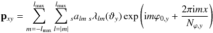 (1)and spherical harmonic analysis (or forward SHT):
 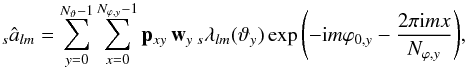 (2)where
  and wy are quadrature weights.
Both transforms can be subdivided into two stages:  Equations (3) and (6) can be computed using fast Fourier transforms (FFTs), while Eqs. (4) and (5), which represent the bulk of the computational load, are the main target for optimised implementation in libsharp.
3. Technical improvements
3.1. General remarks
As the implementation language for the new library, ISO C99 was chosen. This version of the C language standard is more flexible than the C89 one adopted for libpsht and has gained ubiquitous compiler support by now. Most notably, C99 allows definition of new variables anywhere in the code, which improves readability and eliminates a common source of programming mistakes. It also provides native data types for complex numbers, which allows for a more concise notation in many places. However, special care must be taken not to make use of these data types in the library’s public interface, since this would prevent interoperability with C++ codes (because C++ has a different approach to complex number support). Fortunately, this drawback can be worked around fairly easily.
A new approach was required for dealing with the growing variety of instruction sets for arithmetic operations, such as traditional scalar instructions, SSE2 and AVX. Rewriting the library core for each of these alternatives would be cumbersome and error-prone. Instead we introduced the concept of a generic “vector” type containing a number of double-precision IEEE values and defined a set of abstract operations (basic arithmetics, negation, absolute value, multiply-accumulate, min/max, comparison, masking and blending) for this type. Depending on the concrete instruction set used when compiling the code, these operations are then expressed by means of the appropriate operators and intrinsic function calls. The only constraint on the number of values in the vector type is that it has to be a multiple of the underlying instruction set’s native vector length (1 for scalar arithmetic, 2 for SSE2, 4 for AVX).
Using this technique, adding support for new vector instruction sets is straightforward and carries little risk of breaking existing code. As a concrete example, support for the FMA4 instructions present in AMD’s Bulldozer CPUs was added and successfully tested in less than an hour.
3.2. Improved loop structure
After publication of SHT implementations, which perform significantly better than libpsht, especially for s = 0 transforms (Seljebotn 2012; Schaeffer 2013), it became obvious that some bottleneck must be present in libpsht’s implementation. This was identified with libpsht’s approach of first computing a whole l-vector of  in one go, storing it to main memory, and afterwards re-reading it sequentially whenever needed. While the l-vectors are small enough to fit into the CPU’s Level-1 cache, the store and load operations nevertheless caused some latency. For s = 0 transforms with their comparatively low arithmetic operation count (compared to the amount of memory accesses), this latency could not be hidden behind floating point operations and so resulted in a slow-down. This is the most likely explanation for the observation that libpsht’s s = 0 SHTs have a much lower FLOP rate compared to those with s ≠ 0.
It is possible to avoid the store/load overhead for the by applying each value immediately after it has been computed, and discarding it as soon as it is not needed any more. This approach is reflected in the loop structure shown in Figs. 1 and 2, which differs from the one in Reinecke (2011) mainly by the fusion of the central loops over l.
In this context another question must be addressed: the loops marked as “SSE/AVX” in both figures are meant to be executed in “blocks”, i.e. by processing several y indices simultaneously. The block size is equivalent to the size of the generic vector type described in Sect. 3.1. The best value for this parameter depends on hardware characteristics of the underlying computer and therefore cannot be determined a priori. Libsharp always uses a multiple of the system’s natural vector length and estimates the best value by running quick measurements whenever a specific SHT is invoked for the first time. This auto-tuning step approximately takes a tenth of a wall-clock second.
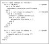 |
Fig. 1 Schematic loop structure of libsharp’s shared-memory synthesis code. |
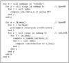 |
Fig. 2 Schematic loop structure of libsharp’s shared-memory analysis code. |
Due to the changed central loop of the SHT implementation, it is no longer straightforward to support multiple simultaneous transforms with differing spins and/or directions, as libpsht did – this would lead to a combinatorial explosion of loop bodies that have to be implemented. Consequently, libsharp, while still supporting simultaneous SHTs, restricts them to have the same spin and direction. Fortunately, this is a very common case in many application scenarios.
3.3. Polar optimisation
As previously mentioned in Reinecke (2011), much CPU time can be saved by simply not computing terms in Eqs. (4)and (5)for which  is so small that their contribution to the result lies well below the numerical accuracy. Since this situation occurs for rings lying close to the poles and high values of m, Schaeffer (2013) referred to it as “polar optimisation”.
To determine which terms can be omitted, libsharp uses the approach described in Prézeau & Reinecke (2010). In short, all terms for which  (7)are skipped. The parameter T is tunable and determines the overall accuracy of the result. Libsharp models it as
 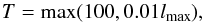 (8)which has been verified to produce results equivalent to those of SHTs without polar optimisation.
4. Added functionality
4.1. SHTs with arbitrary spin
While the most widely used SHTs in cosmology are performed on quantities of spins 0 and 2 (i.e. sky maps of Stokes I and Q/U parameters), there is also a need for transforms at other spins. Lensing computations require SHTs of spin-1 and spin-3 quantities (see, e.g., Lewis 2005). The most important motivation for high-spin SHTs, however, are all-sky convolution codes (e.g. Wandelt & Górski 2001; Prézeau & Reinecke 2010) and deconvolution map-makers (e.g. Keihänen & Reinecke 2012). The computational cost of these algorithms is dominated by calculating expressions of the form 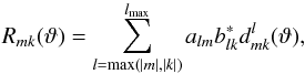 (9)where a and b denote two sets of spherical harmonic coefficients (typically of the sky and a beam pattern) and d are the Wigner d matrix elements. These expressions can be interpreted and solved efficiently as a set of (slightly modified) SHTs with spins ranging from 0 to kmax ≤ lmax, which in today’s applications can take on values much higher than 2.
As was discussed in Reinecke (2011), the algorithms used by libpsht for spin-1 and spin-2 SHTs become inefficient and inaccurate for higher spins. To support such transforms in libsharp, another approach was therefore implemented, which is based on the recursion for Wigner d matrix elements presented in Prézeau & Reinecke (2010).
Generally, the spin-weighted spherical harmonics are related to the Wigner d matrix elements via  (10)(Goldberg et al. 1967). It is possible to compute the
  using a three-term recursion in l very similar to that for the scalar Ylm(ϑ):
 ![Mathematical equation: \begin{eqnarray} &&\left[ \cos\vartheta - \frac{mm^\prime}{l(l+1)}\right] d^{l}_{mm^\prime}(\vartheta) = \frac{\sqrt{(l^2-m^2)(l^2-{m^\prime}^2)}}{l(2l+1)}d^{l-1}_{mm^\prime}(\vartheta) \nonumber \\ &&\hspace{0.9cm}+\frac{\sqrt{[(l+1)^2-m^2][(l+1)^2-{m^\prime}^2]}}{(l+1)(2l+1)}d^{l+1}_{mm^\prime}(\vartheta) \end{eqnarray}](/articles/aa/full_html/2013/06/aa21494-13/aa21494-13-eq35.png) (11)(Kostelec & Rockmore 2008). The terms depending only on l, m, and m′ can be re-used for different colatitudes, so that the real cost of a recursion step is two additions and three multiplications.
(11)(Kostelec & Rockmore 2008). The terms depending only on l, m, and m′ can be re-used for different colatitudes, so that the real cost of a recursion step is two additions and three multiplications.
In contrast to the statements made in McEwen & Wiaux (2011), this recursion is numerically stable when performed in the direction of increasing l; see, e.g., Sect. 5.1.2 for a practical confirmation. It is necessary, however, to use a digital floating-point representation with enhanced exponent range to avoid underflow during the recursion, as is discussed in some detail in Prézeau & Reinecke (2010).
4.2. Distributed memory parallelisation
When considering that, in current research, the required band limit for SHTs practically never exceeds lmax = 104, it seems at first glance unnecessary to provide an implementation supporting multiple nodes. Such SHTs fit easily into the memory of a single typical compute node and are carried out within a few seconds of wall clock time. The need for additional parallelisation becomes apparent, however, as soon as the SHT is no longer considered in isolation, but as a (potentially small) part of another algorithm, which is libsharp’s main usage scenario. In such a situation, large amounts of memory may be occupied by data sets unrelated to the SHT, therefore requiring distribution over multiple nodes. Moreover, there is sometimes the need for very many SHTs in sequence, e.g. if they are part of a sampling process or an iterative solver. Here, the parallelisation to a very large number of CPUs may be the only way of reducing the time-to-solution to acceptable levels. Illustrative examples for this are the Commander code (Eriksen et al. 2008) and the artDeco deconvolution mapmaker (Keihänen & Reinecke 2012); for the processing of high-resolution Planck data, the latter is expected to require over 100GB of memory and several hundred CPU cores.
Libsharp provides an interface that allows collective execution of SHTs on multiple machines with distributed memory. It makes use of the MPI1 interface to perform the necessary inter-process communication.
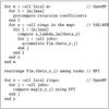 |
Fig. 3 Schematic loop structure of libsharp’s distributed-memory synthesis code. |
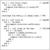 |
Fig. 4 Schematic loop structure of libsharp’s distributed-memory analysis code. |
In contrast to the standard, shared-memory algorithms, it is the responsibility of the library user to distribute map data and alm over the individual computers in a way that ensures proper load balancing. A very straightforward and reliable way to achieve this is a “round robin” strategy: assuming N computing nodes, the map is distributed such that node i hosts the map rings i, i + N, i + 2N, etc. (and their counterparts on the other hemisphere). Similarly, for the spherical harmonic coefficients, node i would hold all alm for m = i, i + N, i + 2N, etc. Other efficient distribution strategies do of course exist and may be advantageous, depending on the circumstances under which libsharp is called. The only requirement the library has is that the alm are distributed by m and that the map is distributed by rings, as described in Figs. 3 and 4.
The SHT algorithm for distributed memory architectures is analogous to the one used in the S2HAT package2 and first published in Szydlarski et al. (2013); its structure is sketched in Figs. 3 and 4. In addition to the S2HAT implementation, the SHT will be broken down into smaller chunks if the average number of map rings per MPI task exceeds a certain threshold. This is analogous to the use of chunks in the scalar and OpenMP-parallel implementations and reduces the memory overhead caused by temporary variables.
It should be noted that libsharp supports hybrid MPI and OpenMP parallelisation, which allows, e.g., running an SHT on eight nodes with four CPU cores each, by specifying eight MPI tasks, each of them consisting of four OpenMP threads. In general, OpenMP should be preferred over MPI whenever shared memory is available (i.e. at the computing node level), since the OpenMP algorithms contain dynamic load balancing and have a smaller communication overhead.
4.3. Map synthesis of first derivatives
Generating maps of first derivatives from a set of alm is closely related to performing an SHT of spin 1. A specialised SHT mode was added to libsharp for this purpose; it takes as input a set of spin-0 alm and produces two maps containing ∂f/∂ϑ and ∂f/(∂ϕsinϑ), respectively.
4.4. Support for additional spherical grids
Direct support for certain classes of spherical grids has been extended in comparison to libpsht; these additions are listed below in detail. It must be stressed, however, that libsharp can – very much as libpsht does – perform SHTs on any iso-latitude grid with equidistant pixels on each ring. This very general class of pixelisations includes, e.g., certain types of partial spherical coverage. For these general grids, however, the user is responsible for providing correct quadrature weights when performing a spherical harmonic analysis.
4.4.1. Extended support for ECP grids
Libpsht provides explicit support for HEALPix grids, Gauss-Legendre grids, and a subset of equidistant cylindrical projection (ECP) grids. The latter are limited to an even number of rings at the colatitudes ![Mathematical equation: \begin{equation} \vartheta_n=\frac{(n+0.5)\pi}{N}, \quad n \in [0;N-1]\text{.} \end{equation}](/articles/aa/full_html/2013/06/aa21494-13/aa21494-13-eq47.png) (12)The associated quadrature weights are given by Fejér’s first rule (Fejér 1933; Gautschi 1967).
(12)The associated quadrature weights are given by Fejér’s first rule (Fejér 1933; Gautschi 1967).
Libsharp extends ECP grid support to allow even and odd numbers of rings, as well as the colatitude distributions ![Mathematical equation: \begin{equation} \vartheta_n=\frac{n\pi}{N}\text{, }\quad n \in [1;N-1] \end{equation}](/articles/aa/full_html/2013/06/aa21494-13/aa21494-13-eq48.png) (13)(corresponding to Fejér’s second rule), and
(13)(corresponding to Fejér’s second rule), and ![Mathematical equation: \begin{equation} \vartheta_n=\frac{n\pi}{N}\text{, }\quad n \in [0;N] \end{equation}](/articles/aa/full_html/2013/06/aa21494-13/aa21494-13-eq49.png) (14)(corresponding to Clenshaw-Curtis quadrature). This last pixelisation is identical to the one adopted in Huffenberger & Wandelt (2010).
(14)(corresponding to Clenshaw-Curtis quadrature). This last pixelisation is identical to the one adopted in Huffenberger & Wandelt (2010).
Accurate computation of the quadrature weights for these pixelisations is nontrivial; libsharp adopts the FFT-based approach described in Waldvogel (2006) for this purpose.
4.4.2. Reduced Gauss-Legendre grid
The polar optimisation described in Sect. 3.3 implies that it is possible to reduce the number of pixels per ring below the theoretically required value of 2lmax + 1 close to the poles. Equation (7)can be solved for m (at a given s, lmax and ϑ), and using 2m + 1 equidistant pixels in the corresponding map ring results in a pixelisation that can represent a band-limited function up to the desired precision, although it is no longer exact in a mathematical sense. If this number is further increased to the next number composed entirely of small prime factors (2, 3, and 5 are used in libsharp’s case), this has the additional advantage of allowing very efficient FFTs.
Libsharp supports this pixel reduction technique in the form of a thinned-out Gauss-Legendre grid. At moderate to high resolutions (lmax > 1000), more than 30% of pixels can be saved, which can be significant in various applications.
It should be noted that working with reduced Gauss-Legendre grids, while saving considerable amounts of memory, does not change SHT execution times significantly; all potential savings are already taken into account, for all grids, by libsharp’s implementation of polar optimisation.
4.5. Adjoint and real SHTs
Since Eq. (1)is a linear transform, we can introduce the notation  (15)for a vector a of spherical harmonic coefficients and corresponding vector p of pixels. Similarly, one can write Eq. (2)as
  (16)where W is a diagonal matrix of quadrature weights. When including SHTs as operators in linear systems, one will often need the adjoint spherical harmonic synthesis, Y†, and the adjoint spherical harmonic analysis, WY. For instance, if a is a random vector with covariance matrix C in the spherical harmonic domain, then its pixel representation Ya has the covariance matrix YCY†. Multiplication by this matrix requires the use of the adjoint synthesis, which corresponds to analysis with a different choice of weights. Libsharp includes routines for adjoint SHTs, which is more user-friendly than having to compensate for the wrong choice of weights in user code, and also avoids an extra pass over the data.
For linear algebra computations, the vector a must also include alm with m < 0, even if libsharp will only compute the coefficients for m ≥ 0. The use of the real spherical harmonics convention is a convenient way to include negative m without increasing the computational workload by duplicating all coefficients. For the definition we refer to the appendix of de Oliveira-Costa et al. (2004). The convention is supported directly in libsharp, although with a restriction in the storage scheme: The coefficients for m < 0 must be stored in the same locations as the corresponding imaginary parts of the complex coefficients, so that the pattern in memory is [al,m,al, − m].
5. Evaluation
Most tests were performed on the SuperMUC Petascale System located at the Leibniz-Rechenzentrum Garching. This system consists of nodes containing 32GB of main memory and 16 Intel Xeon E5-2680 cores running at 2.7GHz. The exception is the comparison with Wavemoth, which was performed on the Abel cluster at the University of Oslo on very similar hardware; Xeon E5-2670 at 2.6 GHz.
The code was compiled with gcc version 4.7.2. The Intel compiler (version 12.1.6) was also tested, but produced slightly inferior code.
Except where noted otherwise, test calculations were performed using the reduced Gauss-Legendre grid (see Sect. 4.4.2) to represent spherical map data. This was done for the pragmatic purpose of minimising the tests’ memory usage, which allowed going to higher band limits in some cases, as well as to demonstrate the viability of this pixelisation.
The band limits adopted for the tests all obey lmax = 2n − 1 with n ∈N (except for those presented in Sect. 5.2.2). This is done in analogy to most other papers on the subject, but leads to some unfamiliar numbers especially at very high lmax.
The number of cores used for any particular run always is a power of 2.
5.1. Accuracy tests
5.1.1. Comparison with other implementations
The numerical equivalence of libsharp’s SHTs to existing implementations was verified by running spherical harmonic synthesis transforms on a Gauss-Legendre grid at lmax = 50 and spins 0, 1, and 2 with both libsharp and libpsht, and comparing the results. The differences of the results lay well within the expected levels of numerical errors caused by the finite precision of IEEE numbers. Spherical harmonic analysis is implicitly tested by the experiments in the following sections.
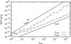 |
Fig. 5 Maximum and rms errors for inverse/forward spin = 0 SHT pairs at different lmax. |
5.1.2. Evaluation of SHT pairs
To test the accuracy of libsharp’s transforms, sets of spin = 0 alm coefficients were generated by setting their real and imaginary parts to numbers drawn from a uniform random distribution in the range [− 1; 1[ (with exception of the imaginary parts for m = 0, which have to be zero for symmetry reasons). This data set was transformed onto a reduced Gauss-Legendre grid and back to spherical harmonic space again, resulting in âlm.
The rms and maximum errors of this inverse/forward transform pair can be written as  Figure 5 shows the measured errors for a wide range of band limits. As expected, the numbers are close to the accuracy limit of double precision IEEE numbers for low lmax; rms errors increase roughly linearly with the band limit, while the maximum error seems to exhibit an lmax3/2 scaling. Even at lmax = 262 143 (which is extremely high compared to values typically required in cosmology), the errors are still negligible compared with the uncertainties in the input data in today’s experiments.
Analogous experiments were performed for spins 2 and 37, with very similar results (not shown).
5.2. Performance tests
Determining reliable execution times for SHTs is nontrivial at low band limits, since intermittent operating system activity can significantly distort the measurement of short time scales. All libsharp timings shown in the following sections were obtained using the following procedure: the SHT pair in question is executed repeatedly until the accumulated wall-clock time exceeds 2 s. Then the shortest measured wall-clock time for synthesis and analysis is selected from the available set.
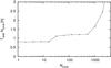 |
Fig. 6 Strong-scaling scenario: accumulated wall-clock time for a spin = 2 SHT pair with lmax = 16 383 run on various numbers of cores. |
5.2.1. Strong-scaling test
To assess strong-scaling behaviour (i.e. run time scaling for a given problem with fixed total workload), a spin = 2 SHT with lmax = 16 383 was carried out with differing degrees of parallelisation. The accumulated wall-clock time of these transforms (synthesis + analysis) is shown in Fig. 6. It is evident that the scaling is nearly ideal up to 16 cores, which implies that parallelisation overhead is negligible in this range. Beyond 16 cores, MPI communication has to be used for inter-node communication, and this most likely accounts for the sudden jump in accumulated time. At even higher core counts, linear scaling is again reached, although with a poorer proportionality factor than in the intra-node case. Finally, for 1024 and more cores, the communication time dominates the actual computation, and scalability is lost.
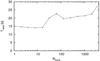 |
Fig. 7 Weak-scaling scenario: wall-clock time for a spin = 0 SHT pair run on various numbers of cores, with constant amount of work per core (lmax(N) = 4096N1/3 − 1). |
5.2.2. Weak-scaling test
Weak-scaling behaviour of the algorithm is investigated by choosing problem sizes that keep the total work per core constant, in contrast to a fixed total workload. Assuming an SHT complexity of  , the band limits were derived from the employed number of cores N via lmax(N) = 4096N1/3 − 1. The results are shown in Fig. 7. Ideal scaling corresponds to a horizontal line. Again, the transition from one to several computing nodes degrades performance, whereas scaling on a single node, as well as in the multi-node range, is very good. By keeping the amount of work per core constant, the breakdown of scalability is shifted to 4096 cores, compared with 1024 in the strong-scaling test.
It is interesting to note that the scaling within a single node is actually slightly superlinear; this is most likely because in this setup, the amount of memory per core decreases with increasing problem size, which in turn can improve the amount of cache re-use and reduce memory bandwidth per core.
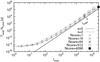 |
Fig. 8 Accumulated wall-clock time for spin = 0 and spin = 2 SHT pairs at a wide range of different band limits. For every run the number of cores was chosen sufficiently small to keep parallelisation overhead low. |
5.2.3. General scaling and efficiency
The preceding two sections did not cover cases with small SHTs. This scenario is interesting, however, since in the limit of small lmax those components of the SHT implementation with complexities lower than (like the FFT steps of Eqs. (3) and (6)) may begin to dominate execution time. Figure 8 shows the total wall-clock time for SHT pairs over a very wide range of band limits; to minimise the impact of communication, the degree of parallelisation was kept as low as possible for the runs in question. As expected, the lmax3 scaling is a very good model for the execution times at lmax ≥ 511. Below this limit, the FFTs, precomputations for the spherical harmonic recursion, memory copy operations and other parts of the code begin to dominate.
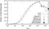 |
Fig. 9 Fraction of theoretical peak-performance reached by various SHT pairs. For every run the number of cores was chosen sufficiently small to keep parallelisation overhead low. |
In analogy to one of the tests described in Reinecke (2011), we computed a lower limit for the number of executed floating-point operations per second in libsharp’s SHTs and compared the result with the theoretical peak performance achievable on the given hardware, which is eight operations per clock cycle (four additions and four multiplications) or 21.6 GFlops/s per core. Figue 9 shows the results. In contrast to libpsht, which reached approximately 22% for s = 0 and 43% for s = 2, both scalar and tensor harmonic transforms exhibit very similar performance levels and almost reach 70% of theoretical peak in the most favourable regime, thanks to the changed structure of the inner loops. For the lmax range that is typically required in cosmological applications, performance exceeds 50% (even when MPI is used), which is very high for a practically useful algorithm on this kind of computer architecture.
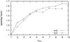 |
Fig. 10 Relative speed-up when performing several SHTs simultaneously, compared with sequential execution. The SHT had a band limit of lmax = 8191. |
5.2.4. Multiple simultaneous SHTs
The computation of the coefficients accounts for roughly half the arithmetic operations in an SHT. If several SHTs with identical grid geometry and band limit are computed simultaneously, it is possible to re-use these coefficients, thereby reducing the overall operation count. Figure 10 shows the speed-ups compared to sequential execution for various scenarios, which increase with the number of transforms and reach saturation around a factor of 1.6. This value is lower than the naïvely expected asymptotic factor of 2 (corresponding to avoiding half of the arithmetic operations), since the changed algorithm requires more memory transfers between Level-1 cache and CPU registers and therefore operates at a lower percentage of theoretical peak performance. Nevertheless, running SHTs simultaneously is evidently beneficial and should be used whenever possible.
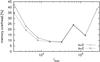 |
Fig. 11 Relative memory overhead, i.e. the fraction of total memory that is not occupied by input and output data of the SHT. For low lmax this is dominated by the program binary, for high lmax by temporary arrays. |
Performance comparison with other implementations at lmax = 2047, ncore = 1.
5.2.5. Memory overhead
Especially at high band limits, it is important that the SHT library does not consume a large amount of main memory, to avoid memory exhaustion and subsequent swapping or code crashes. Libsharp is designed with the goal to keep the size of its auxiliary data structures much lower than the combined size of any SHT’s input and output arrays. A measurement is shown in Fig. 11. Below the lowest shown band limit of 2047, memory overhead quickly climbs to almost 100%, since in this regime memory consumption is dominated by the executable and the constant overhead of the communication libraries, which on the testing machine amounts to approximately 50MB. In the important range (lmax ≥ 2047), memory overhead lies below 45%.
5.2.6. Comparison with existing implementations
Table 1 shows a performance comparison of synthesis/analysis SHT pairs between libsharp and various other SHT implementations. In addition to the already mentioned shtns, Wavemoth, S2HAT and libpsht codes, we also included spinsfast (Huffenberger & Wandelt 2010), SSHT (McEwen & Wiaux 2011) and Glesp (Doroshkevich et al. 2005) in the comparison. All computations shared a common band limit of 2047 and were executed on a single core, since the corresponding SHTs are supported by all libraries and are very likely carried out with a comparatively high efficiency by all of them. The large overall number of possible parameters (lmax, spin, number of simultaneous transforms, degree and kind of parallelisation, choice of grid, etc.) prevented a truly comprehensive study.
Overall, libsharp’s performance is very satisfactory and exhibits speed-ups of more than an order of magnitude in several cases. The table also demonstrates libsharp’s flexibility, since it supports all of the other codes’ “native” grid geometries, which is required for direct comparisons.
The three last columns list time ratios measured under different assumptions: RAVX reflects values that can be expected on modern (2012 and later) AMD/Intel CPUs supporting AVX, RSSE2 applies to older (2001 and later) CPUs with the SSE2 instruction set. Rscalar should be used for CPUs from other vendors like IBM or ARM, since libsharp does not yet support vectorisation for these architectures.
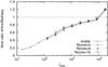 |
Fig. 12 Performance comparison between libsharp and shtns for varying lmax and number of OpenMP threads. Note that reduced autotuning was used for shtns at lmax = 16 383 (see text). |
Figure 12 shows the relative performance of identical SHT pairs on a full Gauss-Legendre grid with s = 0 for libsharp and shtns. For these measurements the benchmarking code delivered with shtns was adjusted to measure SHT times in a similar fashion as was described above. The plotted quantity is shtns wall-clock time divided by libsharp wall-clock time for varying lmax and number of OpenMP threads. It is evident that shtns has a significant advantage for small band limits (almost an order of magnitude) and maintains a slight edge up to lmax = 8191. It must be noted, however, that the measured times do not include the overhead for auto-tuning and necessary precalculations, which in the case of shtns are about an order of magnitude more expensive than the SHTs themselves. As a consequence, its performance advantage only pays off if many identical SHT operations are performed within one run. The origin of shtns’s performance advantage has not been studied in depth; however, a quick analysis shows that the measured time differences scale roughly like lmax2, so the following explanations are likely candidates:
-
libsharp performs all of its precomputations as part of the time-measured SHT;
libsharp’s flexibility with regard to pixelisation and storage arrangement of input and output data requires some additional copy operations;
at low band limits the inferior performance of libsharp’s FFT implementation has a noticeable impact on overall run times.
For lmax = 16 383, the time required by the default shtns autotuner becomes very long (on the order of wall-clock hours), so that we decided to invoke it with an option for reduced tuning. It is likely a consequence of this missed optimisation that, at this band limit, libsharp is the better-performing code.
6. Conclusions
Judging from the benchmarks presented in the preceding section, the goals that were set for the libsharp library have been reached: it exceeds libpsht in terms of performance, supports recent developments in microprocessor technology, allows using distributed memory systems for a wider range of applications, and is slightly easier to use. On the developer side, the modular design of the code makes it much more straightforward to add support for new instruction sets and other functionality.
In some specific scenarios, especially for SHTs with comparatively low band limits, libsharp does not provide the best performance of all available implementations, but given its extreme flexibility concerning grid types and the memory layout of its input/output data, as well as its compactness (≈8000 lines of portable and easily maintainable source code without external dependencies), this compromise certainly seems acceptable.
The library has been successfully integrated into version 3.1 of the HEALPix C++ and Fortran packages. There also exists an experimental version of the SSHT3 package with libsharp replacing the library’s original SHT engine. Libsharp is also used as SHT engine in an upcoming version of the Python package NIFTy4 for signal inference (Selig et al. 2013). Recently, the total convolution code conviqt (Prézeau & Reinecke 2010), which is a central component of the Planck simulation pipeline (Reinecke et al. 2006), has been updated and is now based
on libsharp SHTs. There are plans for a similar update of the artDeco deconvolution map maker (Keihänen & Reinecke 2012).
A potential future field of work is porting libsharp to Intel’s “many integrated cores” architecture5, once sufficient compiler support for this platform has been established. The hardware appears to be very well suited for running SHTs, and the porting by itself would provide a welcome test for the adaptability of the library’s code design.
Acknowledgments
We thank our referee Nathanaël Schaeffer for his constructive remarks and especially for pointing out a missed optimisation opportunity in our shtns installation, which had a significant effect on some benchmark results. M.R. is supported by the German Aeronautics Center and Space Agency (DLR), under program 50-OP-0901, funded by the Federal Ministry of Economics and Technology. D.S.S. is supported by the European Research Council, grant StG2010-257080. The presented benchmarks were performed as project pr89yi at the Leibniz Computing Center Garching.
References
- de Oliveira-Costa, A., Tegmark, M., Zaldarriaga, M., & Hamilton, A. 2004, Phys. Rev. D, 69, 063516 [NASA ADS] [CrossRef] [Google Scholar]
- Doroshkevich, A. G., Naselsky, P. D., Verkhodanov, O. V., et al. 2005, Int. J. Mod. Phys. D, 14, 275 [NASA ADS] [CrossRef] [Google Scholar]
- Eriksen, H. K., Jewell, J. B., Dickinson, C., et al. 2008, ApJ, 676, 10 [NASA ADS] [CrossRef] [Google Scholar]
- Fejér, L. 1933, Mathematische Zeitschrift, 37, 287 [CrossRef] [Google Scholar]
- Gautschi, W. 1967, SIAM J. Numerical Analysis, 4, 357 [NASA ADS] [CrossRef] [Google Scholar]
- Goldberg, J. N., Macfarlane, A. J., Newman, E. T., Rohrlich, F., & Sudarshan, E. C. G. 1967, J. Math. Phys., 8, 2155 [NASA ADS] [CrossRef] [Google Scholar]
- Huffenberger, K. M., & Wandelt, B. D. 2010, ApJS, 189, 255 [NASA ADS] [CrossRef] [Google Scholar]
- Keihänen, E., & Reinecke, M. 2012, A&A, 548, A110 [NASA ADS] [CrossRef] [EDP Sciences] [Google Scholar]
- Kostelec, P., & Rockmore, D. 2008, J. Fourier Analysis and Applications, 14, 145 [CrossRef] [Google Scholar]
- Lewis, A. 2005, Phys. Rev. D, 71, 083008 [NASA ADS] [CrossRef] [Google Scholar]
- McEwen, J. D., & Wiaux, Y. 2011, IEEE Trans. Signal Proc., 59, 5876 [Google Scholar]
- Prézeau, G., & Reinecke, M. 2010, ApJS, 190, 267 [NASA ADS] [CrossRef] [Google Scholar]
- Reinecke, M. 2011, A&A, 526, A108 [NASA ADS] [CrossRef] [EDP Sciences] [Google Scholar]
- Reinecke, M., Dolag, K., Hell, R., Bartelmann, M., & Enßlin, T. A. 2006, A&A, 445, 373 [NASA ADS] [CrossRef] [EDP Sciences] [Google Scholar]
- Schaeffer, N. 2013, Geochem. Geophys. Geosyst., 14 [Google Scholar]
- Selig, M., Bell, M. R., Junklewitz, H., et al. 2013, IEEE Trans. Inf. Theory, submitted [arXiv:1301.4499] [Google Scholar]
- Seljebotn, D. S. 2012, ApJS, 199, 5 [NASA ADS] [CrossRef] [Google Scholar]
- Szydlarski, M., Esterie, P., Falcou, J., Grigori, L., & Stompor, R. 2013, Concurrency and Computation: Practice and Experience [Google Scholar]
- Waldvogel, J. 2006, BIT Numerical Mathematics, 46, 195 [CrossRef] [Google Scholar]
- Wandelt, B. D., & Górski, K. M. 2001, Phys. Rev. D, 63, 123002 [NASA ADS] [CrossRef] [Google Scholar]
All Tables
All Figures
|
Fig. 1 Schematic loop structure of libsharp’s shared-memory synthesis code. |
| In the text | |
|
Fig. 2 Schematic loop structure of libsharp’s shared-memory analysis code. |
| In the text | |
|
Fig. 3 Schematic loop structure of libsharp’s distributed-memory synthesis code. |
| In the text | |
|
Fig. 4 Schematic loop structure of libsharp’s distributed-memory analysis code. |
| In the text | |
|
Fig. 5 Maximum and rms errors for inverse/forward spin = 0 SHT pairs at different lmax. |
| In the text | |
|
Fig. 6 Strong-scaling scenario: accumulated wall-clock time for a spin = 2 SHT pair with lmax = 16 383 run on various numbers of cores. |
| In the text | |
|
Fig. 7 Weak-scaling scenario: wall-clock time for a spin = 0 SHT pair run on various numbers of cores, with constant amount of work per core (lmax(N) = 4096N1/3 − 1). |
| In the text | |
|
Fig. 8 Accumulated wall-clock time for spin = 0 and spin = 2 SHT pairs at a wide range of different band limits. For every run the number of cores was chosen sufficiently small to keep parallelisation overhead low. |
| In the text | |
|
Fig. 9 Fraction of theoretical peak-performance reached by various SHT pairs. For every run the number of cores was chosen sufficiently small to keep parallelisation overhead low. |
| In the text | |
|
Fig. 10 Relative speed-up when performing several SHTs simultaneously, compared with sequential execution. The SHT had a band limit of lmax = 8191. |
| In the text | |
|
Fig. 11 Relative memory overhead, i.e. the fraction of total memory that is not occupied by input and output data of the SHT. For low lmax this is dominated by the program binary, for high lmax by temporary arrays. |
| In the text | |
|
Fig. 12 Performance comparison between libsharp and shtns for varying lmax and number of OpenMP threads. Note that reduced autotuning was used for shtns at lmax = 16 383 (see text). |
| In the text | |
Current usage metrics show cumulative count of Article Views (full-text article views including HTML views, PDF and ePub downloads, according to the available data) and Abstracts Views on Vision4Press platform.
Data correspond to usage on the plateform after 2015. The current usage metrics is available 48-96 hours after online publication and is updated daily on week days.
Initial download of the metrics may take a while.