| Issue |
A&A
Volume 554, June 2013
|
|
|---|---|---|
| Article Number | A61 | |
| Number of page(s) | 12 | |
| Section | Stellar structure and evolution | |
| DOI | https://doi.org/10.1051/0004-6361/201321467 | |
| Published online | 04 June 2013 | |
Are there tangled magnetic fields on HgMn stars?⋆
1
Department Physics and Astronomy Uppsala University,
Box 516,
75120
Uppsala,
Sweden
e-mail:
This email address is being protected from spambots. You need JavaScript enabled to view it.
2
Institute of Astrophysics, Georg-August University,
Friedrich-Hund-Platz 1,
37077
Göttingen,
Germany
3
Department of Physics and Astronomy, Rice
University, 6100 Main
Street, Houston,
TX
77005,
USA
4
Sterrewacht Leiden, Universiteit Leiden,
Niels Bohrweg 2, 2333 CA
Leiden, The
Netherlands
5
Space Telescope Science Institute, 3700 San Martin Dr, Baltimore, MD
21211,
USA
Received: 13 March 2013
Accepted: 21 April 2013
Abstract
Context. Several recent spectrophotometric studies failed to detect significant global magnetic fields in late-B HgMn chemically peculiar stars, but some investigations have suggested the presence of strong unstructured or tangled fields in these objects.
Aims. We used detailed spectrum synthesis analysis to search for evidence of tangled magnetic fields in high-quality observed spectra of eight slowly rotating HgMn stars and one normal late-B star. We also evaluated recent sporadic detections of weak longitudinal magnetic fields in HgMn stars based on the moment technique.
Methods. Our spectrum synthesis code calculated the Zeeman broadening of metal lines in HARPS spectra, assuming an unstructured, turbulent magnetic field. A simple line formation model with a homogeneous radial field distribution was applied to assess compatibility between previous longitudinal field measurements and the observed mean circular polarization signatures.
Results. Our analysis of the Zeeman broadening of magnetically sensitive spectral lines reveals no evidence of tangled magnetic fields in any of the studied HgMn or normal stars. We infer upper limits of 200–700 G for the mean magnetic field modulus – much smaller than the field strengths implied by studies based on differential magnetic line intensification and quadratic field diagnostics. The new HARPSpol longitudinal field measurements for the extreme HgMn star HD 65949 and the normal late-B star 21 Peg are consistent with zero at a precision of 3–6 G. Re-analysis of our Stokes V spectra of the spotted HgMn star HD 11753 shows that the recent moment technique measurements retrieved from the same data are incompatible with the lack of circular polarization signatures in the spectrum of this star.
Conclusions. We conclude that there is no evidence for substantial tangled magnetic fields on the surfaces of studied HgMn stars. We cannot independently confirm the presence of very strong quadratic or marginal longitudinal fields for these stars, so results from the moment technique are likely to be spurious.
Key words: stars: atmospheres / stars: chemically peculiar / stars: general / stars: magnetic field / polarization
Based on observations collected at the European Southern Observatory, Chile (ESO programmes 084.D-0338, 085.D-0296, 086.D-0240).
© ESO, 2013
1. Introduction
Mercury-manganese (HgMn) stars comprise a group of late-B chemically peculiar stars distinguished by a strong overabundance and an unusual isotopic composition of heavy elements (Adelman et al. 2004; Woolf & Lambert 1999). Many of these stars are slow rotators and members of close spectroscopic binary systems (Abt et al. 2002; Catanzaro & Leto 2004). The properties of HgMn stars facilitate precise chemical abundance analysis of their atmospheres (e.g. Adelman et al. 2006), making them the preferred targets for detailed comparisons of observed surface abundance patterns and predictions from atomic diffusion theory (Michaud et al. 1974; Alecian & Michaud 1981).
The unexpected discovery of low-contrast abundance inhomogeneities on the surfaces of HgMn stars has rekindled interest in the astrophysical processes that operate in these stars (Adelman et al. 2002; Kochukhov et al. 2005, 2011a; Hubrig et al. 2006a). Chemical spots are often found in magnetic B-type (Bp) stars, which overlap with HgMn stars on the H-R diagram. Bp stars possess strong global magnetic fields, which are believed to be responsible for the chemical spot formation (e.g. Michaud et al. 1981). In contrast to this clear link between magnetic fields and chemical spots in Bp stars, no robust and reproducible magnetic field detections have ever been reported for any of the HgMn stars. Moreover, inhomogeneities on HgMn stars evolve with time (Kochukhov et al. 2007; Briquet et al. 2010), possibly indicating a previously unknown time-dependent, non-equilibrium diffusion process (Alecian et al. 2011). This behavior is, again, very different from that of spots on magnetic Bp stars, which are observed to be stable for at least several decades (Adelman et al. 2001).
The possible role of weak magnetic fields in explaining the puzzling surface phenomena observed in HgMn stars is a topic of ongoing debate. The literature contains claims of magnetic field detections based on low- and high-resolution spectropolarimetric observations (Hubrig et al. 2006b, 2010, 2012). However, many other detailed circular polarization studies of individual spotted HgMn stars revealed no magnetic field signatures in spectral line profiles (Wade et al. 2006; Folsom et al. 2010; Makaganiuk et al. 2011a, 2012; Kochukhov et al. 2011a). Similar null results were also reported by several spectropolarimetric surveys that included a large number of HgMn-type stars (Shorlin et al. 2002; Aurière et al. 2010; Makaganiuk et al. 2011b). These studies established an upper limit from a few tens of G to just a few G for the mean longitudinal magnetic field in HgMn stars.
The failure of spectropolarimetric studies to unambiguously detect the fields in HgMn stars may be attributed to the complexity of the surface magnetic field topologies (e.g. Hubrig 1998). Indeed, spectropolarimetry and, especially, the mean longitudinal magnetic field diagnostic is only sensitive to the line-of-sight magnetic field component. Theoretically, the net line-of-sight magnetic field can be close to zero if many regions of opposite polarity are present on the stellar surface. Highly structured magnetic field topologies can reduce the Stokes V signatures in spectral line profiles below the detection threshold. On the other hand, field orientation has a relatively minor effect on magnetic broadening and splitting, so this diagnostic can reveal complex magnetic fields invisible to spectropolarimetry. This type of analysis has yielded a number of surprisingly high magnetic field estimates for HgMn stars. For instance, on the basis of studying the differential magnetic intensification of Fe ii lines, Hubrig et al. (1999) and Hubrig & Castelli (2001) concluded that some HgMn stars possess complex or “tangled” magnetic fields stronger than 2 kG. A complementary quadratic magnetic field diagnostic method based on the comparison of magnetic broadening in spectral lines with different Zeeman splitting patterns suggested the presence of even stronger, 2–8 kG, magnetic fields in HgMn stars (Mathys & Hubrig 1995; Hubrig et al. 2012).
Both the magnetic intensification and quadratic field diagnostic methods rely on a number of simplifying assumptions about the spectral line formation in magnetic field. These methods were originally developed for intensity spectra with limited wavelength coverage and for spectropolarimetric observations with moderate resolution and relatively low signal-to-noise ratio (S/N). Modern échelle spectra of HgMn stars provide access to numerous magnetically sensitive lines that can be analyzed using sophisticated theoretical tools. The goal of our paper is to probe the existence of complex magnetic fields in HgMn stars by taking advantage of the high-resolution, high S/N observations and using accurate methods to model magnetic radiative transfer. We also critically examine spectropolarimetric magnetic field detections that seem to contradict our null results for a few HgMn stars (Makaganiuk et al. 2011a,b, 2012).
Atmospheric parameters and rotational velocities of HgMn stars.
Observational data and results of the magnetic field analysis of HgMn stars.
The rest of the paper is organized as follows. Section 2 presents our spectroscopic and spectropolarimetric observations and discusses corresponding analysis methods. Results of the magnetic field search using circular polarization measurements, differential magnetic intensification, and Zeeman broadening of spectral lines are reported in Sect. 3. Finally, Sect. 4 compares our results with the outcome of previous investigations and assesses implications of our study for the general question of the presence of magnetic fields in HgMn stars.
2. Methods
2.1. Observations and data reduction
We analyze spectra of HgMn stars obtained with the circular polarimetric mode (Snik et al. 2011; Piskunov et al. 2011) of the HARPS spectrometer (Mayor et al. 2003) installed at the 3.6-m ESO telescope in La Silla. Most observations were obtained during several observing runs in 2010. The acquisition and reduction of these data was described in detail by Makaganiuk et al. (2011b,a, 2012). We also obtained new circular polarization observations of the HgMn star HD 65949 and analyzed spectra of the normal late-B star HD 209459, which was observed together with the HgMn stars from our sample but was not studied by Makaganiuk et al.
The HARPSpol instrument records spectra in the wavelength range 3780–6913 Å with an 80 Å gap around 5300 Å. All stars in our study were observed using the circular polarization analyzer. Observations of each star were typically split into four sub-exposures between which the quarter-wave retarder plate was rotated in 90° steps relative to the beamsplitter. The spectra were extracted and calibrated using a dedicated version of the reduce pipeline (Piskunov & Valenti 2002). The Stokes I spectrum was obtained by averaging the right- and left-hand polarized spectra from all sub-exposures of a given star. The Stokes V and diagnostic null spectra were derived by combining the extracted spectra according to the “ratio” spectropolarimetric demodulation method (Donati et al. 1997; Bagnulo et al. 2009). Analysis of the emission lines in the ThAr comparison spectra showed that the resolving power of HARPS in polarimetric mode is R = λ/Δλ = 109 000 with about 1–2% variation across the échelle format.
Subtle Zeeman broadening due to a weak and complex magnetic field can be reliably detected only for very slowly rotating stars. Therefore, we selected a small number of sharp-lined targets out of the full sample of HgMn stars examined in the survey by Makaganiuk et al. (2011b). Our primary targets include 7 HgMn stars with vesini ≤ 2 km s-1: HD 35548, HD 65949, HD 71066, HD 175640, HD 178065, HD 186122, and HD 193452. For comparison, we also analyzed two stars with projected rotational velocities in the range of 4–6 km s-1: HD 78316 (κ Cnc) and HD 209459 (21 Peg). Table 1 summarizes alternative designations, atmospheric parameters and literature information on the rotational velocities of our program stars.
Preliminary continuum normalization of Stokes I spectra was performed by consecutively applying the blaze function, an empirical response function, and smooth fit corrections as described by Makaganiuk et al. (2011b). The resulting continuum normalization has a precision of approximately 0.5%. The final zeroth-order correction to the continuum was applied as part of the modeling of intensity profiles of individual spectral lines described below (Sect. 3.3).
Characteristics of the HARPSpol observations of 9 program stars are provided in Table 2. We list the UT dates of individual observations, the corresponding heliocentric Julian dates, the total exposure time, and the peak S/N per pixel measured at λ ≈ 5200 Å. Two observations were obtained for 21 Peg. Both were used to measure the mean longitudinal magnetic field (Sect. 3.1), but only the higher quality one was employed for the Stokes I Zeeman broadening analysis (Sect. 3.3).
2.2. Multi-line polarization analysis
A search for weak magnetic field signatures in high-resolution stellar Stokes V spectra is greatly facilitated by a multi-line analysis. In this study we used the least-squares deconvolution (LSD) code developed by Kochukhov et al. (2010). The LSD method, originally introduced by Donati et al. (1997), combines information from all suitable stellar absorption lines under the assumption of self-similarity of the line profile shapes and a linear addition of overlapping lines. Kochukhov et al. (2010) showed that these assumptions are adequate for weak and moderately strong magnetic fields and that the mean longitudinal magnetic field inferred from the Stokes V LSD profiles is not affected by systematic biases.
In this study we applied the LSD analysis to our new spectropolarimetric observations of HD 65949 and HD 209459. For the remaining targets the LSD longitudinal field measurements were published by Makaganiuk et al. (2011b). For completeness, Table 2 reproduces these measurements. The line lists necessary for applying LSD were obtained from the VALD database (Kupka et al. 1999), using atmospheric parameters listed in Table 1 and adopting chemical abundances from the studies by Cowley et al. (2010) and Fossati et al. (2009) for HD 65949 and HD 209459, respectively. In total, we used 500–600 lines deeper than 10% of the continuum for each star. The application of LSD increased the S/N of the Stokes V profiles by a factor of ≈6. Section 3.1 describes the analysis of the LSD profiles of HD 65949 and HD 209459.
2.3. Magnetic intensification and broadening of spectral lines
The Zeeman effect produces intensification, broadening, and splitting of a spectral line depending on its effective Landé factor and the magnetic splitting pattern. However, unless the field is very strong and the Zeeman splitting can be resolved and measured directly, there are few, if any, reliable model-independent methods to derive magnetic field intensity from the Stokes I spectra. In particular, as we will show below, such techniques as differential line intensification and quadratic field diagnostic are prone to biases and lead to contradictory results for late-B stars. In this situation, detailed spectrum synthesis is the only robust way to detect and measure magnetic fields with strengths below 1–2 kG (Kochukhov et al. 2002, 2006; Johns-Krull 2007). Refined analysis of high-resolution spectra of bright stars can even reveal fields in the 400–500 G range (Anderson et al. 2010).
Here we use the synmast magnetic spectrum synthesis code (Kochukhov et al. 2010) to simulate the effects of different magnetic field geometries on the profiles of magnetically sensitive metal lines. This code calculates the four Stokes parameter spectra for a homogeneous magnetic field distribution characterized by the three vector components specified in the stellar coordinate system (see Kochukhov 2007) or for a turbulent magnetic field as described below. These calculations are based on the llmodels model atmospheres (Shulyak et al. 2004), computed for the stellar parameters given in Table 1 taking individual abundances of the program stars into account. We set the microturbulent velocity to zero, since HgMn stars are known to lack signatures of turbulence in their atmospheres (Landstreet et al. 2009).
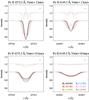 |
Fig. 1 Effect of the turbulent magnetic field on the Fe ii 4273.3 and 6149.3 Å lines. The solid curves show synthetic profiles for the field strengths ranging from 0 to 3 kG and for vesini = 2 and 10 km s-1. The dotted lines show the difference between the magnetic and non-magnetic profiles, offset vertically by 1.2. The error bar in the upper right corner of each panel corresponds to the S/N of 200:1. |
As mentioned in the introduction, previous studies of HgMn stars could not unambiguously detect Zeeman-induced polarization in spectral lines. Even if we believe a few disputed detections, the polarimetrically-inferred magnetic fields in HgMn stars typically do not exceed ~100 G. At the same time, multi-kG fields were inferred from the analysis of intensity spectra of the same or similar stars. These vastly different field strength estimates can be reconciled only if the fields are arranged on the stellar surfaces in a highly structured, complex configuration. To model such fields we use the concept of an isotropic, turbulent magnetic field (Landi Degl’Innocenti & Landolfi 2004), which implies magnetic field parameters that are uncorrelated on the characteristic scale of radiative transfer. A turbulent field represents an opposite extreme compared to an organized, large-scale magnetic field topology. Yet, it is the only known magnetic field model satisfying the observational requirement of giving a noticeable Zeeman broadening and intensification in the intensity spectra without producing a detectable circular polarization.
In general, the isotropic, turbulent magnetic field is characterized by some distribution of the magnetic field modulus, F(Bt). For this magnetic field topology, the polarized radiative transfer equation terms that depend on the field orientation average to zero, yielding null emergent QUV spectra but retaining the magnetic field effects in Stokes I. We implemented this model in the synmast code assuming, as a first approximation, that the entire stellar surface is covered by the magnetic field with a strength ⟨ Bt ⟩. The disk-integrated spectra for arbitrary vesini are then produced from the intensity calculations at several limb angles, similar to a non-magnetic spectrum synthesis (Kochukhov 2007).
Figure 1 illustrates the effect of a turbulent magnetic field on the Fe ii 4273.3 (z = 2.15, pseudo-triplet splitting) and 6149.3 Å (z = 1.35, doublet splitting) spectral lines. These calculations were done for the Teff = 12 000 K, log g = 4.0 model atmosphere and a spectral resolution R = 109 000. As one can see from this figure, for a very low vesini, both lines show detectable profile distortions for ⟨ Bt ⟩ ≥ 0.5–1.0 kG fields. Starting from ~2 kG, the partially-resolved Zeeman splitting becomes obvious in the Fe ii 6149.3 Å line. For higher projected rotational velocities a stronger field is required to produce significant line profile distortions. Based on these calculations, we conclude that, provided vesini can be independently estimated from magnetically insensitive lines, it is possible to detect kG-strength tangled magnetic fields using magnetically sensitive spectral lines in S/N ≥ 200, R ≥ 105 observations of slowly rotating late-B stars.
2.4. Modeling of circular polarization profiles
Historically, the efforts to detect magnetic fields in early-type chemically peculiar stars mostly relied on the longitudinal field diagnostic (e.g. Borra & Landstreet 1980; Mathys 1991). However, modern availability of the high-quality mean Stokes V profiles enables several other field detection and assessment methods. For instance, Petit & Wade (2012) demonstrated how a useful estimate of the surface dipolar field strength can be obtained from the LSD Stokes V profiles without complete rotational phase coverage. Shultz et al. (2012) used a similar polarization modeling approach to test compatibility of their high-resolution Stokes V observations with the magnetic field models derived solely from the ⟨ Bz ⟩ measurements. Here we apply a similar technique to assess the circular polarization signatures expected for individual ⟨ Bz ⟩ detections reported in the literature.
To model the observed LSD Stokes I and V profiles, we use the polarization spectrum synthesis method described by Petit & Wade (2012). The local intensity profile is represented by a Gaussian function while the Stokes V is given by the scaled derivative of the Gaussian according to the well-known weak-field approximation formula (Landi Degl’Innocenti & Landolfi 2004). The wavelength and effective Landé factor required by this approximation are given by the respective mean values for the LSD mask. The Stokes I and V spectra are obtained by numerical integration of these local profiles over the visible stellar hemisphere for a given magnetic field geometry. For the calculations presented in this paper, we adopted a homogeneous radial field distribution with the strength adjusted to match a particular ⟨ Bz ⟩ value. Other free parameters of the model (vesini and line depth) were obtained by fitting the observed Stokes I profile.
Although not as realistic as e.g. dipolar field, such schematic field model has the advantage of producing the same basic anti-symmetric Stokes V profile shape independently of the viewing angle. Experimenting with different magnetic field distributions, we found that a uniform radial field provides the most conservative estimate of the circular polarization amplitude for a given ⟨ Bz ⟩. In other words, any other surface magnetic field distribution must produce a stronger Stokes V signature for the same ⟨ Bz ⟩. This is illustrated in Fig. 2, where we show the Stokes V profiles computed for a perpendicular dipolar field and for radial fields with the same ⟨ Bz ⟩ at each rotational phase. Evidently, the radial field distributions yield a lower amplitude of the circular polarization signal. This difference is small for very low vesini but then quickly increases for larger projected rotational velocities because of the crossover effect (Mathys 1995a). Thus, one can ascertain that the Stokes V profiles corresponding to a homogeneous radial field provide a robust lower limit on the circular polarization signal that must accompany a given ⟨ Bz ⟩ measurement.
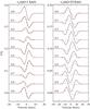 |
Fig. 2 Comparison of the Stokes V signatures for the dipolar field topology with i = β = 90° (solid lines) and for a homogeneous radial field distribution (dashed lines) scaled to give the same mean longitudinal field at each rotational phase. The left and right panels show results for vesini = 1 and 10 km s-1, respectively. The Stokes V spectra are offset vertically according to the stellar rotational phase. |
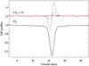 |
Fig. 3 LSD Stokes I and V profiles for HD 65949. The mean polarization profile is offset vertically and expanded by a factor of 10 relative to Stokes I. The dashed lines show the circular polarization signatures for ⟨ Bz ⟩ = −77 and −290 G, corresponding to the range of the FORS1/2 longitudinal field detections reported by Hubrig et al. (2012). |
3. Results
3.1. Non-detection of the longitudinal magnetic field in HD 65949 and HD 209459
The outcome of our single Stokes V observation of the extreme HgMn star HD 65949 (Cowley et al. 2010) is illustrated in Fig. 3. The LSD Stokes V profile has no polarization signature stronger than 10-3. The mean longitudinal magnetic field, ⟨ Bz ⟩ = −2.8 ± 4.6 G, inferred from the first moment of the circular polarization profile is also formally consistent with zero. Thus, we conclude that there is no evidence of a magnetic field on HD 65949.
Hubrig et al. (2012) published five FORS1/2 longitudinal magnetic field measurements of HD 65949 with typical error bars of 20–60 G. Four of their ⟨ Bz ⟩ values, distributed over seven years, suggest a magnetic field detection in the range −77 G to −290 G. Bagnulo et al. (2012) reanalyzed the FORS1 observation from which the last (and the strongest) of these measurements was derived, finding ⟨ Bz ⟩ = −42 ± 79 G. They conclude that in this and many other cases, the FORS detections of weak magnetic fields are not reliable.
We used the method described in Sect. 2.4 to predict the Stokes V signatures corresponding to the ⟨ Bz ⟩ values reported by Hubrig et al. (2012). As demonstrated by the dashed lines in Fig. 3, a longitudinal field at the level of −77 to −290 G should produce a prominent polarization signature, readily detectable with the LSD profile quality achieved in our observations. It is highly improbable that this huge difference between the predicted and observed polarization signature is due to rotational modulation. Thus, the HARPSpol data are incompatible with previous claims of the longitudinal magnetic field detections in HD 65949.
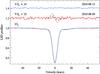 |
Fig. 4 LSD Stokes I and V profiles for the two HARPSpol observations of HD 209459. The mean polarization profiles are offset vertically and expanded by a factor of 10 relative to Stokes I. The dashed lines show the circular polarization signatures for ⟨ Bz ⟩ = 53 and 99 G, corresponding to the range of the longitudinal field detections claimed by Hubrig et al. (2012) from the same observational data. |
Two HARPSpol spectropolarimetric observations are available for the superficially normal late-B star HD 209459 (21 Peg). The LSD Stokes I and V profiles derived from these spectra are presented in Fig. 4. No evidence of the Zeeman Stokes V signatures can be found above the noise level of 1.7 × 10⁻³ for the first (9 Aug. 2010) and 8.7 × 10⁻⁴ for the second (13 Aug. 2010) observation. The corresponding longitudinal magnetic field is −2.2 ± 6.0 G and −4.6 ± 3.1 G, respectively. Thus, it is unlikely that 21 Peg possesses a large-scale field stronger than a few G.
Contrary to these results, Hubrig et al. (2012) reported a 50–100 G longitudinal field based on the moment technique analysis (Mathys 1991) of the same HARPSpol spectra of 21 Peg. Magnetic field was presumably found in the lines of Ti, Cr, and Fe, which comprise 80% of the features included in our LSD line mask for this star. Surprisingly, these detections were reported only for the lower quality spectrum but not for the higher quality one obtained four days later. The minimum Stokes V signature corresponding to the ⟨ Bz ⟩ measurements reported by Hubrig et al. (2012) significantly exceeds the noise level of the LSD Stokes V profiles (see Fig. 4). The lower S/N observation is incompatible with the predicted polarization signature for ⟨ Bz ⟩ = 53 G at the confidence level of ≫99.9% according to a χ2 probability analysis. The lack of polarization signal in the data is therefore grossly inconsistent with the longitudinal field detections obtained for 21 Peg using the moment technique.
3.2. Magnetic intensification of the Fe II 6147 and 6149 Å spectral lines
The singly ionized iron absorption lines at 6147.7 and 6149.3 Å share the same upper atomic energy level and have nearly identical oscillator strengths. However, their Zeeman splitting patterns are very different: the 6147.7 Å line splits in two π and four σ components whereas the 6149.3 Å line has two σ components coinciding in wavelength with the pair of π components. As a result, the latter line exhibits a simple doublet Zeeman splitting pattern, which makes this line particularly useful for direct measurements of the mean magnetic field modulus in slowly rotating Ap stars (Mathys et al. 1997), despite its relatively small effective Landé factor (z = 1.35).
The two Fe ii lines have very similar intensity in normal stars. On the other hand, in the presence of the magnetic field with a strength above a few kG, the Fe ii 6147.7 Å line experiences a stronger magnetic intensification compared to the 6149.3 Å line. Mathys (1990) and Mathys & Lanz (1992) noted that in the field strength interval from 3 to 5 kG the normalized equivalent width difference of these lines, ΔWλ/ ⟨ Wλ ⟩ ≡ 2(W6147 − W6149)/(W6147 + W6149), follows an approximately linear trend with mean magnetic field modulus. Mathys & Lanz (1992) warned against extrapolating this relation to weaker fields. Nevertheless, several subsequent studies of Am and HgMn stars ascribed 5–10% intensification of 6147.7 relative to 6149.3 Å to the presence of 2–3 kG magnetic fields with a complex structure (Lanz & Mathys 1993; Hubrig et al. 1999; Hubrig & Castelli 2001).
A handful of Ap stars have fields stronger than ~5 kG, causing the Fe ii 6147.7 and 6149.3 Å lines to exhibit incomplete Paschen-Back splitting (Mathys 1990), which has been investigated in detail (Takeda 1991; Stift et al. 2008). The formation of these lines in weak magnetic fields has not been studied as thoroughly. Takeda (1991) carried out theoretical disk-center line profile and equivalent width calculations neglecting magneto-optical effects. Part of his conclusions were based on a simplified analytical treatment of polarized radiative transfer (PRT) in a Milne-Eddington atmosphere. Subsequently, Nielsen & Wahlgren (2002) presented another set of differential intensification calculations based on mimicking PRT by adding individual Zeeman components to the input line list for regular unpolarized spectrum synthesis. Both studies suggested significant non-linearities in the weak-field behavior of the magnetic intensification.
Here we investigated behavior of the Fe ii 6147.7 and 6149.3 Å lines for different magnetic field geometries using accurate numerical PRT calculations discussed in Sect. 2.3. Adopting the oscillator strengths log gf = −2.827 and −2.841 (Raassen & Uylings 1998) for the 6147.7 and 6149.3 Å line, respectively, we computed the relative intensification factors and examined the resulting line profiles for the 0–4 kG magnetic field range. These calculations took the incomplete Paschen-Back effect in the Fe ii lines into account, although deviations from the linear Zeeman splitting are relatively small in the range of field strengths considered here.
Figure 5 shows ΔWλ/ ⟨ Wλ ⟩ as a function of the magnetic field strength for the homogeneous radial, azimuthal, and turbulent fields. Evidently, the weak-field behavior of the Fe ii line pair is complex and does not follow a linear extrapolation from the strong-field regime. In the field interval 1–2 kG significant “negative” intensification is expected for the azimuthal and turbulent magnetic fields. Formally, the same intensification factor is obtained in the absence of the field and for fields as strong as 1.5–3.0 kG. This means that comparing only the equivalent widths of these two Fe ii lines will not yield an unambiguous detection of a magnetic field below 2.5–3.0 kG because their relative intensification curve is strongly non-linear in this regime and depends on an a priori unknown field topology.
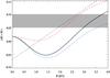 |
Fig. 5 Relative intensification of the Fe ii 6147.7 and 6149.3 Å lines as a function of the magnetic field strength. Different curves show results for turbulent (solid line), radial (dashed line), and azimuthal (dash-dotted line) magnetic field. The dotted line shows an empirical relation for strong-field Ap stars (Mathys & Lanz 1992). The shaded rectangular region corresponds to the intensification measurements reported for HgMn stars in the literature. |
In previous studies of HgMn stars, the intensification factors ΔWλ/ ⟨ Wλ ⟩ at the level of 5–10% were attributed to the presence of magnetic field. Figure 5 shows that this interpretation requires the mean field intensity to be above 2 kG for radial and above 3 kG for turbulent and azimuthal fields, respectively. Our calculations show that for such fields the Zeeman broadening and splitting of spectral lines is considerable and should be easily detectable with R ≥ 105 observations of sharp-lined HgMn stars. This is illustrated in Fig. 6, which compares the observed spectra of the HgMn stars from our sample with the PRT calculations for the stellar parameters Teff = 12 000 K, log g = 4.0, [Fe] = + 0.5, B = 2.5 kG, and for vesini = 1.5 km s-1 typical of our target stars. Independently of the magnetic field geometry, a noticeable broadening of the Fe ii 6147.7 Å line and a splitting of the 6149.3 Å line occurs for the magnetic field intensity exceeding 1.5–2.0 kG. But the actual high-resolution observed spectra of the HgMn stars analyzed here and presented in previous studies (e.g. see Fig. 1 in Hubrig & Castelli 2001) conspicuously lack any signs of the magnetically-induced spectral line profile distortions. The lack of such distortions rules out field moduli above 1.5–2.0 kG.
Figure 6 also shows that the Hg ii 6149.5 Å line is present in most of our stars and is particularly prominent HD 65949 due to its high mercury overabundance. For stars with vesini exceeding a few km s-1 this feature will blend the Fe ii 6149.3 line, compromising the equivalent width analysis (see also Takada-Hidai & Jugaku 1992).
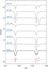 |
Fig. 6 Profiles of the Fe ii 6147.7 and 6149.3 Å lines in the spectra of HgMn stars. The observed spectra are offset vertically for clarity. The unshifted spectra show theoretical calculations for 2.5 kG radial (dashed line) and turbulent (solid line) magnetic field. The dash-dotted line corresponds to non-magnetic theoretical spectrum. The vertical dotted lines indicate central wavelengths of the Fe ii lines. The bottom plot schematically illustrates the Zeeman splitting patterns of the two Fe ii lines. |
Thus, we conclude that magnetic field detections based on comparing the equivalent widths of the Fe ii 6147.7 and 6149.3 Å lines are ambiguous and potentially misleading. In fact, for the slowly rotating stars, magnetic intensification is less informative than the profile shapes of the same spectral lines. The observed Fe ii line profiles of all 7 HgMn stars with vesini ≤ 2 km s-1 are incompatible with previous studies that interpreted 6147.7 vs. 6149.3 Å equivalent widths in terms of magnetic fields.
3.3. Upper limits on tangled magnetic fields
The Zeeman broadening analysis of each target star was carried out in several steps. First, we calculated a grid of synthetic spectra for different turbulent magnetic field strengths covering the entire HARPS wavelength range. For these calculations we adopted the model atmosphere parameters listed in Table 1 and compiled information on stellar abundances from previous studies. The atomic line data were extracted from the VALD database. Using this grid of synthetic spectra, we identified two groups of unblended spectral lines with a different response to magnetic field. We used the first group of about 10–15 spectral lines with small effective Landé factors (typically z ≤ 0.5) to determine vesini. The central wavelengths and Landé factors of these lines are given in Table 3. We used a least-squares routine to fit each spectral line individually, allowing stellar radial velocity and elemental abundance to vary. The last column of Table 1 reports the mean and standard deviation of our projected rotational velocities.
For the two SB2 stars in our sample, HD 35548 and HD 78316 (κ Cnc), special effort was made to avoid spectral regions affected by the absorption lines of the companion. We also corrected synthetic spectra for the continuum dilution by the secondary stars using the light ratios derived by Ryabchikova et al. (1998) and Dolk et al. (2002) for HD 78316 and HD 35548, respectively.
Spectral lines used for broadening analysis.
Next we analyzed in detail a smaller (5–10) set of magnetically sensitive spectral lines (see Table 3). Most of them had z ≥ 1.5, but a few, like Fe ii 4385.387 Å and Fe ii 6149.3 Å, provided useful constraints on the magnetic field despite a relatively small Landé factor, due to their unusual Zeeman splitting patterns. The list of usable spectral lines was dominated by Fe ii, but varied from star to star depending on the chemical composition, blending, and the quality of observations. Several magnetically sensitive lines, notably Fe ii 4273.3 and 6149.3 Å, were analyzed in each star. We avoided very strong Fe ii lines, such as 4923.9 and 5018.4 Å, which might be affected by NLTE effects in the line core.
For each magnetically sensitive line we performed a series of least-squares fits for different vesini and turbulent magnetic field strengths. These parameters were varied in steps of 0.1 km s-1 and 50 G within ±1 km s-1 around the previously determined vesini and for ⟨ Bt ⟩ between 0 and 1000 G, respectively. Since we considered only the magnetic distortion of the spectral line shapes, the element abundance was adjusted individually for each vesini-⟨ Bt ⟩ pair.
Figure 7 presents examples of our spectrum synthesis fits for different magnetic field strengths. It shows a pair of low-z Fe ii lines together with two magnetically sensitive lines in the spectrum of HD 71066. One can see that, after adjusting the line strength, it is possible to obtain an excellent fit for both groups of lines with zero magnetic field intensity. On the other hand, if the field strength is increased to 1 kG, the two low-z lines are not affected while the calculated profiles of the magnetically sensitive lines become broader than the observations.
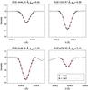 |
Fig. 7 Comparison of observations and synthetic spectra computed for Fe ii lines of different magnetic sensitivity in the spectrum of HD 71066. Observations are shown with symbols. Filled circles indicate the wavelength interval considered for the least-squares fit. The solid line represents synthetic spectrum in the absence of magnetic field. The dashed line corresponds to the calculations for 1 kG turbulent field. |
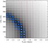 |
Fig. 8 Derivation of the upper limit on the turbulent magnetic field strength in HD 71066 using the Fe ii 4273.3 Å line. The χ2 of the fit (background image) is shown as a function of ⟨ Bt ⟩ and vesini. The squares indicate parameter combinations compatible with observations at the 95% confidence level. The crosses show ⟨ Bt ⟩-vesini pairs consistent with the projected rotational velocity (vertical lines) determined from the magnetically insensitive spectral lines. |
To obtain quantitative constraints on the turbulent magnetic field strength we examined the fit χ2 as a function of vesini and ⟨ Bt ⟩, as illustrated in Fig. 8. The confidence level of the fit was characterized by the χ2 probability function, Pχ2. For a typical spectral line with a triplet-like Zeeman splitting, the effects of a weak magnetic field and rotational Doppler broadening largely compensate each other, so an adequate fit can be achieved with different combinations of vesini and ⟨ Bt ⟩. This degeneracy can be lifted by considering the vesini derived from magnetically insensitive lines. Assuming that the probability of finding a particular value of vesini follows a Gaussian distribution, Pg, with the center and width given by the mean vesini and the corresponding error (see Table 1), we constructed the total probability function Ptot(vesini, ⟨ Bt ⟩ ) = Pχ2Pg. In this way, we combined information about the fit quality for a particular magnetically sensitive line with the vesini constraint from lines not affected by magnetic field.
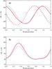 |
Fig. 10 Effect of Y spots on the determination of the mean longitudinal magnetic field of the HgMn star HD 11753. The curves show ⟨ Bz ⟩ as a function of rotation phase for the Y map derived by Makaganiuk et al. (2012) (thick lines) and for a uniform element distribution (thin lines). a) Calculations for the dipolar field topology with a polar strength of 500 G, obliquity β = 90°, and two different orientations with respect to the reference rotation phase (solid and dashed lines). b) Calculations for the radial magnetic field map scaled according to the Y abundance distribution. |
A few spectral lines have Zeeman splitting patterns that are wide doublets, making it possible to distinguish magnetic broadening from rotational Doppler broadening. This allowed us to disentangle vesini and ⟨ Bt ⟩ even for a relatively low magnetic field strength. Figure 9 provides an example of this situation for the Fe ii 6149.3 Å line in the spectrum of HD 71066. In this case the observations are clearly not compatible with the slow rotation/strong field scenario because the Zeeman splitting cannot mimic rotational broadening.
We analyzed 8 HgMn and one normal late-B star. None of these stars require the presence of a magnetic field to match the observed profiles of spectral lines with different magnetic sensitivity. Adopting a confidence level of 95%, we inferred upper limits for the turbulent magnetic field in each star, using 2−3 spectral lines that provide the best constraint. These upper limits are reported in the last column of Table 2. Typically, we rule out fields above 200–300 G for the HgMn stars with low projected rotational velocities (vesini ≤ 2 km s-1). A higher limit of 500 G was obtained for one sharp-lined HgMn star, HD 178065 because low iron abundance weakens many useful Fe ii diagnostic features (see Fig. 6). For the two more rapidly rotating stars, HD 78316 (κ Cnc) and HD 209459 (21 Peg), we constrained ⟨ Bt ⟩ to be below 600–700 G. Therefore, the principal conclusion of this section is that the line broadening in high-resolution spectra of the target stars is incompatible with the idea of ubiquitous presence of multi-kG complex magnetic fields in the HgMn-star atmospheres.
4. Discussion
4.1. Tangled magnetic fields in HgMn stars
Our detailed spectrum synthesis analysis shows that modern R > 105 spectra could detect the weak magnetic broadening that would be caused by 1–2 kG unstructured fields in slowly rotating HgMn stars. However, observed profiles of lines with different magnetic sensitivity rule out tangled fields stronger than a few hundred G in the atmospheres of the HgMn stars studied here.
We showed that some claims of strong complex fields in HgMn stars, in particular those that interpret equivalent widths of Fe ii 6147.7 and 6149.3 Å in terms of differential magnetic intensification, relied on incorrect assumptions about spectral line formation and therefore cannot be substantiated.
Our magnetic line formation calculations suggest that unambiguous detection of magnetic intensification with this Fe ii line pair requires a field so strong that Zeeman splitting would be obvious in slowly rotating stars. Of course, the latter effect can be masked by line broadening in faster rotators, but in such stars the differential intensification method is not reliable anyway due to line blending problems (Takada-Hidai & Jugaku 1992).
Highly sensitive analyses of the Stokes V LSD profiles of HgMn stars (see Sect. 3.1 and Makaganiuk et al. 2011b) place stringent upper limits on the mean longitudinal magnetic field. The non-detection of the circular polarization signals in high-resolution spectra also rules out the presence of weak complex magnetic fields topologically similar to those found in active late-type stars because the signatures of latter fields are readily detectable with HARPSpol and other modern spectropolarimeters (e.g. Kochukhov et al. 2011b). Thus, it should be realized that the putative tangled fields of HgMn stars must be substantially weaker and/or more complex than the dynamo fields of cool stars to evade detections with modern high-resolution spectropolarimeters.
Recently, weak sub-G fields have been detected on Vega and Sirius (Petit et al. 2010, 2011). We cannot rule out such fields on HgMn stars or any other type of intermediate-mass stars. However, such fields would not be dynamically important, and therefore are not capable of providing an explanation for the chemical spot formation in HgMn stars. Thus, for the purpose of understanding the dichotomy between non-magnetic (HgMn, Am) and strongly magnetic (Ap/Bp) intermediate-mass stars, we find no compelling reasons to revise the “non-magnetic” classification of HgMn stars.
4.2. Longitudinal field detections for HgMn stars
Currently, the most precise constraints on magnetic fields in HgMn stars are obtained by applying the LSD technique to high-resolution circular polarization spectra (Aurière et al. 2010; Makaganiuk et al. 2011b; Kochukhov et al. 2011a). However, the null results of the HARPSpol magnetic survey of HgMn stars (Makaganiuk et al. 2011b) and non-detections of the magnetic field in individual objects (Makaganiuk et al. 2011a, 2012) analyzed with the LSD method were recently challenged by Hubrig et al. (2012). These authors re-analyzed the same high-resolution HARPSpol polarization spectra with an alternative moment technique (Mathys 1991) and in a few cases reported 3–4σ detections of 30–100 G longitudinal magnetic fields. Analysis was carried out for individual chemical elements, resulting in ⟨ Bz ⟩ error bars 10–30 G, significantly exceeding those obtained for the same targets by the LSD approach.
Hubrig et al. (2010, 2012) invoked inhomogeneous distributions of chemical elements to explain why the moment analysis of individual elements yields much stronger fields than permitted by the LSD results. These authors suggested that the (unspecified) distribution of spots on HgMn stars enhances the polarization signal for inhomogeneously distributed elements but suppresses the signal for Fe-peak elements that dominate the LSD line mask. However, in the study of the HgMn star HD 11753 Makaganiuk et al. (2012) applied LSD to individual elements, including those with the strongest horizontal abundance gradients, without detecting a field at any epoch. Furthermore, results obtained by Hubrig et al. (2012) for this star seem to contradict their hypothesis because the longitudinal field is fairly coherent for all analyzed elements, including Fe, at the two phases with claimed magnetic field detections. In addition, discrepancies between the application of the moment method and the LSD polarization analyses were also found for non-peculiar stars without chemical spots, e.g. for 21 Peg (Sect. 3.1) and for pulsating B-type stars (Shultz et al. 2012).
In general, one does not expect topologically simple and low-contrast chemical spots on HgMn stars to have a large effect on the longitudinal magnetic field measurements. Using results from a Doppler imaging analysis of HD 11753 (Makaganiuk et al. 2012), we assessed in detail the influence of inhomogeneous Y distribution on ⟨ Bz ⟩ measurements obtained from the spectral lines of this element. Theoretical Stokes I and V spectra were computed using the Invers10 code (Piskunov & Kochukhov 2002) for the Y map derived by Makaganiuk et al. (2012) and for a homogeneous distribution of this element. For these calculations we adopted the dipolar field topology with a polar strength Bp = 500 G, obliquity β = 90°, and two different azimuth angles, ϕ = 0° and 90°. The resulting ⟨ Bz ⟩ curves obtained from the synthetic spectra are presented in Fig. 10a. It is evident that even for Y, which shows the largest abundance contrast across the surface of HD 11753, the non-uniform element distribution results in no more than 10–20% change of ⟨ Bz ⟩. Depending on the field geometry, one may expect reduction or amplification of the longitudinal field inferred from the lines of a non-uniformly distributed element.
In another test calculation we considered an outward-directed radial field with a local intensity that was scaled between 0 and +200 G according to the (logarithmic) abundance of Y. We then compared ⟨ Bz ⟩ curves inferred from synthetic Y lines computed for this field, assuming either a non-uniform or a homogeneous element distribution. Figure 10b demonstrates that with this magnetic field distribution, which perfectly matches the yttrium abundance spots as in the scenarios implied by Hubrig et al. (2010, 2012), we find that ⟨ Bz ⟩ is enhanced by a mere 12% at the phase when Y line strength is at maximum. These calculations confirm that weak chemical inhomogeneities found on HgMn stars do not significantly enhance magnetic field detections and cannot be responsible for the discrepancies between the LSD and moment technique results.
The LSD technique determines the average Stokes V profile, and not just a single scalar quantity, e.g. the mean longitudinal magnetic field. This allows one to reveal topologically complex or crossover magnetic fields, which yield a detectable Zeeman signature even when the first-order moment of Stokes V is negligible. Simultaneously, one can use various objective statistical methods to assess compatibility of the theoretical magnetic field models with the observed LSD profiles (e.g. Shultz et al. 2012; Petit & Wade 2012). Here we used this opportunity to directly test the ⟨ Bz ⟩ moment measurements reported by Hubrig et al. (2012) for HD 11753 and other HgMn stars.
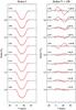 |
Fig. 11 LSD Stokes I (left panel) and V (right panel) profiles of the HgMn star HD 11753. Thin lines show observations by Makaganiuk et al. (2012) obtained during 10 nights, starting on 2010-01-04 (top profile) and ending on 2010-01-14 (bottom profile). The thick curves correspond to the minimum-amplitude Stokes V model profiles reproducing the longitudinal field measurements obtained from the same observational data by Hubrig et al. (2012). Rotational phases are indicated on the left side of each panel. The numbers on the right side of the Stokes V panel report the probability that observations and model profiles are compatible within the error bars. |
Using the LSD line profile modeling method described in Sect. 2.4, we have predicted the minimum amplitude of the mean Stokes V profile for the longitudinal magnetic field measurements published by Hubrig et al. (2012). The comparison between the observed and modeled Stokes I and V profiles of HD 11753 is presented in Fig. 11 for all 10 rotational phases analyzed in the original paper by Makaganiuk et al. (2012). The computed Stokes V signatures correspond to the maximum longitudinal field strength reported by Hubrig et al. (2012) for the same set of rotational phases. The Stokes V panel of this figure reports the false alarm probability (FAP), characterizing the probability that the difference between the observed and model profiles can be attributed to observational noise. For all but two or three cases, ⟨ Bz ⟩ inferred by the moment method is incompatible with the observed LSD profiles. In particular, for the two phases for which Hubrig et al. (2012) claimed 3–4σ field detections (0.789, 0.205), we find FAP < 10-6. There are three more phases (0.891, 0.313, 0.729) when simulated signals are highly improbable (FAP < 10-3). This shows that the high ⟨ Bz ⟩ values reported for HD 11753 by Hubrig et al. (2012) are ruled out by the observed LSD profiles. Similar conclusions can be reached for other HgMn stars observed with HARPSpol (41 Eri, 66 Eri, HD 78316). Applying the same analysis to the LSD Stokes I and V profiles of the binary HgMn star AR Aur (Folsom et al. 2010), we established an upper limit, at the 99% confidence level, of 45 G and 100 G on the absolute value of ⟨ Bz ⟩ for the primary and secondary components, respectively. This agrees well with the non-detection of the longitudinal field by Folsom et al. (2010) but is grossly incompatible with | ⟨ Bz ⟩ | values of up to 560 G for the primary and up to 260 G for the secondary claimed by Hubrig et al. (2010, 2012).
We emphasize that our models of the LSD profiles of HD 11753 and other HgMn stars assume a homogeneous radial field distribution, which corresponds to the smallest possible amplitude of the circular polarization signature for a given ⟨ Bz ⟩. In the presence of stellar rotation with vesini above a few km s-1, any realistic global field configuration, e.g. a dipole, and especially any complex magnetic field distribution will inevitably lead to additional lobes in the Stokes V profile, yielding a much higher peak-to-peak amplitude of the Zeeman signatures for the same ⟨ Bz ⟩. This would make the discrepancy between predicted Stokes V signatures and the actual observations even more dramatic.
What could be the reason for these discrepant longitudinal field measurements, which are often obtained from the same observational material? Part of the disagreement may be related to different reduction methods. Hubrig et al. (2012) analyzed spectra from a generic HARPS pipeline, whereas we analyzed spectra from the reduce code (Piskunov & Valenti 2002) with optimizations designed to yield precise spectropolarimetry. The essential difference between the two reduction procedures is that the polarimetric version of the HARPS pipeline does not include continuum normalization nor the response function correction necessary to compensate for large differences in HARPS fiber throughput. Omitting these steps may lead to a non-negligible spurious continuum polarization. Combined with the longitudinal field measurement technique based on performing a linear least-squares fit (forced through the origin) of the first moment of Stokes V profiles (Mathys 1991), this may result in spurious magnetic field detections.
There could also exist other methodological problems with the applications of the moment technique to weak polarimetric signals. The LSD method has a well-established track record for detecting and characterizing strong (Wade et al. 2000), intermediate (Aurière et al. 2007) and extremely weak (Petit et al. 2010) stellar magnetic fields. It was also thoroughly tested using theoretical polarized spectrum synthesis calculations for a wide range of magnetic field strengths and orientations (Kochukhov et al. 2010). In contrast, the moment technique has been systematically applied only to moderate-quality observations of the strong-field Ap/Bp stars (Mathys 1991; Mathys & Hubrig 1997). It is not immediately obvious that an extension of the moment measurements to very low-amplitude circular polarization signals hidden in the noise is robust, especially when it comes to 3–4σ ⟨ Bz ⟩ measurements that are not accompanied by a definite detection of Stokes V signatures.
To this end, the experience with the FORS low-resolution field detection technique is particularly instructive. Measurements using standard FORS pipeline yielded reasonable results for strong-field Ap stars (Kochukhov & Bagnulo 2006; Landstreet et al. 2007) but, at the same time, suggested detection of weak fields in a variety of objects not known to be magnetic (Hubrig et al. 2009), including HgMn stars (Hubrig et al. 2006b). Very few of these detections were validated by other instruments (Silvester et al. 2009; Shultz et al. 2012). These problematic FORS results were eventually traced to poorly documented subtle details of the data reduction and processing, which led to a systematic underestimation of the uncertainty of derived magnetic field strengths (Bagnulo et al. 2012). The moment technique in the implementation used by Hubrig et al. (2012) appears to suffer a similar pitfall when applied to stars with very weak or absent magnetic fields. Unfortunately, these authors did not provide enough detail to reproduce their analysis step by step.
Based on this assessment, we conclude that there is no convincing evidence of the magnetic fields in HgMn stars from high-resolution circular polarization data. Given controversial results and refuted detections, any claim of a significant longitudinal magnetic field in these stars should be considered with caution, if it is not accompanied by the primary magnetic observable: a non-zero Stokes V signature repeatedly detected in individual spectral lines or in mean line profiles.
4.3. Quadratic fields
The mean quadratic magnetic field, 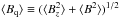 , represents an alternative method of extracting information about stellar magnetic fields from the differential broadening of spectral lines with different magnetic sensitivity. This magnetic field diagnostic technique was introduced by Mathys (1995b) and further improved by Mathys & Hubrig (2006). Quadratic field is derived under simplifying assumptions about line formation expressed as multiple linear regressions of observed second-order moments of line profiles against central wavelength, equivalent width, and Zeeman splitting parameters of spectral lines. The quantity
  derived from observations does not separate contributions of the longitudinal field and the field modulus. Due to its attempt to disentangle multiple broadening agents affecting Stokes I spectra, the quadratic field diagnostic method is considerably more complicated to apply compared to, e.g., the mean longitudinal magnetic field measurements. In practice, it is necessary to use different regression relations for different stars and even for different elements in the same star (Mathys & Hubrig 2006).
Quadratic magnetic fields were systematically measured and interpreted with some success for strong-field Ap stars (Mathys 1995b; Landstreet & Mathys 2000; Bagnulo et al. 2002). At the same time, application of this method to some Ap stars led to occasional controversies since ⟨ Bq ⟩ was found to be much larger than implied by the separate ⟨ Bz ⟩ and ⟨ B ⟩ measurements (Kupka et al. 1996; Kochukhov et al. 2004). Furthermore, Kochukhov (2004) showed that quadratic field can be overestimated by up to 40% if it is derived from the spectral lines of a non-uniformly distributed chemical element.
Based on application of the quadratic field measurement technique, Mathys & Hubrig (1995) claimed the discovery of a remarkably strong magnetic field in the HgMn primary of 74 Aqr. For this star the measurements on two nights gave ⟨ Bq ⟩ = 3.6 kG. Hubrig (1998) also reported 2.7 kG quadratic field in κ Cnc. More recently, the claims of significant quadratic field detections in HgMn stars were repeated by Hubrig et al. (2012), who published ⟨ Bq ⟩ estimates ranging from 1.3 kG in 21 Peg to 6–8 kG in both components of AR Aur. However, no detailed description or illustration of the definitive quadratic field measurements for HgMn stars (as presented by e.g. Mathys & Hubrig 2006, for magnetic Ap stars) can be found in any of these papers. The authors also did not address the biases due to an inhomogeneous element distribution.
In the context of our study, the constraints on turbulent magnetic field strength derived above can be converted to upper limits on the mean quadratic field. For the random-field model considered in our paper,  and ⟨ B2 ⟩ = ⟨ B ⟩ 2, so one can find that ⟨ Bq ⟩ ≈ 1.15 ⟨ Bt ⟩. Taking this into account, our results rule out 1.3 and 2.7 kG quadratic fields obtained in previous studies of 21 Peg and κ Cnc, respectively. No direct comparison can be made for other HgMn stars with the quadratic field detections because their vesini are too large for deriving ⟨ Bt ⟩ with our technique. Nevertheless, we note that detailed spectrum synthesis modeling of the disentangled spectra of the binary components of AR Aur carried out by Folsom et al. (2010) does not support the presence of 6–8 kG tangled magnetic fields, since such fields would have resulted in line strengths that were irreproducible by their non-magnetic spectrum synthesis. Similarly, the detailed abundance analysis and non-magnetic spectrum synthesis fits published for 74 Aqr A by Catanzaro & Leone (2006) contradict the presence of 3.6 kG field in this star.
Thus, at this moment, the quadratic magnetic field detections reported for HgMn stars cannot be independently verified and are likely to be spurious given their disagreement with direct line profile analysis. More information about practical details of the ⟨ Bq ⟩ determination using linear regressions and a comprehensive examination of the limitations of this technique using theoretical spectra is required to assess its reliability and usefulness for HgMn stars.
Acknowledgments
O.K. is a Royal Swedish Academy of Sciences Research Fellow, supported by the grants from Knut and Alice Wallenberg Foundation and Swedish Research Council.
References
- Abt, H. A., Levato, H., & Grosso, M. 2002, ApJ, 573, 359 [NASA ADS] [CrossRef] [Google Scholar]
- Adelman, S. J., Malanushenko, V., Ryabchikova, T. A., & Savanov, I. 2001, A&A, 375, 982 [NASA ADS] [CrossRef] [EDP Sciences] [Google Scholar]
- Adelman, S. J., Gulliver, A. F., Kochukhov, O. P., & Ryabchikova, T. A. 2002, ApJ, 575, 449 [NASA ADS] [CrossRef] [Google Scholar]
- Adelman, S. J., Proffitt, C. R., Wahlgren, G. M., Leckrone, D. S., & Dolk, L. 2004, ApJS, 155, 179 [NASA ADS] [CrossRef] [Google Scholar]
- Adelman, S. J., Caliskan, H., Gulliver, A. F., & Teker, A. 2006, A&A, 447, 685 [NASA ADS] [CrossRef] [EDP Sciences] [Google Scholar]
- Alecian, G., & Michaud, G. 1981, ApJ, 245, 226 [NASA ADS] [CrossRef] [Google Scholar]
- Alecian, G., Stift, M. J., & Dorfi, E. A. 2011, MNRAS, 418, 986 [NASA ADS] [CrossRef] [Google Scholar]
- Anderson, R. I., Reiners, A., & Solanki, S. K. 2010, A&A, 522, A81 [NASA ADS] [CrossRef] [EDP Sciences] [Google Scholar]
- Aurière, M., Wade, G. A., Silvester, J., et al. 2007, A&A, 475, 1053 [NASA ADS] [CrossRef] [EDP Sciences] [Google Scholar]
- Aurière, M., Wade, G. A., Lignières, F., et al. 2010, A&A, 523, A40 [NASA ADS] [CrossRef] [EDP Sciences] [Google Scholar]
- Bagnulo, S., Landi Degl’ Innocenti, M., Landolfi, M., & Mathys, G. 2002, A&A, 394, 1023 [NASA ADS] [CrossRef] [EDP Sciences] [Google Scholar]
- Bagnulo, S., Landolfi, M., Landstreet, J. D., et al. 2009, PASP, 121, 993 [NASA ADS] [CrossRef] [Google Scholar]
- Bagnulo, S., Landstreet, J. D., Fossati, L., & Kochukhov, O. 2012, A&A, 538, A129 [NASA ADS] [CrossRef] [EDP Sciences] [Google Scholar]
- Borra, E. F., & Landstreet, J. D. 1980, ApJS, 42, 421 [NASA ADS] [CrossRef] [Google Scholar]
- Briquet, M., Korhonen, H., González, J. F., Hubrig, S., & Hackman, T. 2010, A&A, 511, A71 [NASA ADS] [CrossRef] [EDP Sciences] [Google Scholar]
- Castelli, F., & Hubrig, S. 2004, A&A, 425, 263 [NASA ADS] [CrossRef] [EDP Sciences] [Google Scholar]
- Castelli, F., Kurucz, R., & Hubrig, S. 2009, A&A, 508, 401 [NASA ADS] [CrossRef] [EDP Sciences] [Google Scholar]
- Catanzaro, G., & Leto, P. 2004, A&A, 416, 661 [NASA ADS] [CrossRef] [EDP Sciences] [Google Scholar]
- Catanzaro, G., & Leone, F. 2006, MNRAS, 373, 330 [NASA ADS] [CrossRef] [Google Scholar]
- Cowley, C. R., Hubrig, S., Palmeri, P., et al. 2010, MNRAS, 405, 1271 [NASA ADS] [Google Scholar]
- Dolk, L., Wahlgren, G. M., Lundberg, H., et al. 2002, A&A, 385, 111 [NASA ADS] [CrossRef] [EDP Sciences] [Google Scholar]
- Donati, J.-F., Semel, M., Carter, B. D., Rees, D. E., & Collier Cameron, A. 1997, MNRAS, 291, 658 [NASA ADS] [CrossRef] [MathSciNet] [Google Scholar]
- Folsom, C. P., Kochukhov, O., Wade, G. A., Silvester, J., & Bagnulo, S. 2010, MNRAS, 407, 2383 [NASA ADS] [CrossRef] [Google Scholar]
- Fossati, L., Ryabchikova, T., Bagnulo, S., et al. 2009, A&A, 503, 945 [NASA ADS] [CrossRef] [EDP Sciences] [Google Scholar]
- Hubrig, S. 1998, Contributions of the Astronomical Observatory Skalnate Pleso, 27, 296 [Google Scholar]
- Hubrig, S., & Castelli, F. 2001, A&A, 375, 963 [NASA ADS] [CrossRef] [EDP Sciences] [Google Scholar]
- Hubrig, S., Castelli, F., & Wahlgren, G. M. 1999, A&A, 346, 139 [NASA ADS] [Google Scholar]
- Hubrig, S., González, J. F., Savanov, I., et al. 2006a, MNRAS, 371, 1953 [NASA ADS] [CrossRef] [Google Scholar]
- Hubrig, S., North, P., Schöller, M., & Mathys, G. 2006b, Astron. Nachr., 327, 289 [NASA ADS] [CrossRef] [Google Scholar]
- Hubrig, S., Schöller, M., Savanov, I., et al. 2009, Astron. Nachr., 330, 708 [NASA ADS] [CrossRef] [Google Scholar]
- Hubrig, S., Savanov, I., Ilyin, I., et al. 2010, MNRAS, 408, L61 [NASA ADS] [CrossRef] [Google Scholar]
- Hubrig, S., González, J. F., Ilyin, I., et al. 2012, A&A, 547, A90 [NASA ADS] [CrossRef] [EDP Sciences] [Google Scholar]
- Johns-Krull, C. M. 2007, ApJ, 664, 975 [NASA ADS] [CrossRef] [Google Scholar]
- Kochukhov, O. 2004, in Magnetic stars, Proc. International Conference, held in the Special Astrophysical Observatory of the Russian AS, August 27–31, 2003, eds. Y. Glagolevskij, D. Kudryavtsev, I. Romanyuk, et al., 64 [Google Scholar]
- Kochukhov, O. 2007, in Physics of Magnetic Stars, eds. I. I. Romanyuk, & D. O. Kudryavtsev, 109 [Google Scholar]
- Kochukhov, O., & Bagnulo, S. 2006, A&A, 450, 763 [NASA ADS] [CrossRef] [EDP Sciences] [Google Scholar]
- Kochukhov, O., Landstreet, J. D., Ryabchikova, T., Weiss, W. W., & Kupka, F. 2002, MNRAS, 337, L1 [NASA ADS] [CrossRef] [Google Scholar]
- Kochukhov, O., Drake, N. A., Piskunov, N., & de la Reza, R. 2004, A&A, 424, 935 [NASA ADS] [CrossRef] [EDP Sciences] [Google Scholar]
- Kochukhov, O., Piskunov, N., Sachkov, M., & Kudryavtsev, D. 2005, A&A, 439, 1093 [NASA ADS] [CrossRef] [EDP Sciences] [Google Scholar]
- Kochukhov, O., Tsymbal, V., Ryabchikova, T., Makaganyk, V., & Bagnulo, S. 2006, A&A, 460, 831 [NASA ADS] [CrossRef] [EDP Sciences] [Google Scholar]
- Kochukhov, O., Adelman, S. J., Gulliver, A. F., & Piskunov, N. 2007, Nature Phys., 3, 526 [Google Scholar]
- Kochukhov, O., Makaganiuk, V., & Piskunov, N. 2010, A&A, 524, A5 [NASA ADS] [CrossRef] [EDP Sciences] [Google Scholar]
- Kochukhov, O., Makaganiuk, V., Piskunov, N., et al. 2011a, A&A, 534, L13 [NASA ADS] [CrossRef] [EDP Sciences] [Google Scholar]
- Kochukhov, O., Makaganiuk, V., Piskunov, N., et al. 2011b, ApJ, 732, L19 [NASA ADS] [CrossRef] [Google Scholar]
- Kupka, F., Ryabchikova, T. A., Weiss, W. W., et al. 1996, A&A, 308, 886 [NASA ADS] [Google Scholar]
- Kupka, F., Piskunov, N., Ryabchikova, T. A., Stempels, H. C., & Weiss, W. W. 1999, A&AS, 138, 119 [NASA ADS] [CrossRef] [EDP Sciences] [MathSciNet] [PubMed] [Google Scholar]
- Landi Degl’Innocenti, E., & Landolfi, M. 2004, ApSS Lib., Polarization in Spectral Lines (Kluwer Academic Publishers), 307 [Google Scholar]
- Landstreet, J. D., & Mathys, G. 2000, A&A, 359, 213 [NASA ADS] [Google Scholar]
- Landstreet, J. D., Bagnulo, S., Andretta, V., et al. 2007, A&A, 470, 685 [NASA ADS] [CrossRef] [EDP Sciences] [Google Scholar]
- Landstreet, J. D., Kupka, F., Ford, H. A., et al. 2009, A&A, 503, 973 [NASA ADS] [CrossRef] [EDP Sciences] [Google Scholar]
- Lanz, T., & Mathys, G. 1993, A&A, 280, 486 [NASA ADS] [Google Scholar]
- Makaganiuk, V., Kochukhov, O., Piskunov, N., et al. 2011a, A&A, 529, A160 [NASA ADS] [CrossRef] [EDP Sciences] [Google Scholar]
- Makaganiuk, V., Kochukhov, O., Piskunov, N., et al. 2011b, A&A, 525, A97 [NASA ADS] [CrossRef] [EDP Sciences] [Google Scholar]
- Makaganiuk, V., Kochukhov, O., Piskunov, N., et al. 2012, A&A, 539, A142 [NASA ADS] [CrossRef] [EDP Sciences] [Google Scholar]
- Mathys, G. 1990, A&A, 232, 151 [NASA ADS] [Google Scholar]
- Mathys, G. 1991, A&AS, 89, 121 [NASA ADS] [Google Scholar]
- Mathys, G. 1995a, A&A, 293, 733 [NASA ADS] [Google Scholar]
- Mathys, G. 1995b, A&A, 293, 746 [NASA ADS] [Google Scholar]
- Mathys, G., & Hubrig, S. 1995, A&A, 293, 810 [NASA ADS] [Google Scholar]
- Mathys, G., & Hubrig, S. 1997, A&AS, 124, 475 [NASA ADS] [CrossRef] [EDP Sciences] [Google Scholar]
- Mathys, G., & Hubrig, S. 2006, A&A, 453, 699 [NASA ADS] [CrossRef] [EDP Sciences] [Google Scholar]
- Mathys, G., & Lanz, T. 1992, A&A, 256, 169 [NASA ADS] [Google Scholar]
- Mathys, G., Hubrig, S., Landstreet, J. D., Lanz, T., & Manfroid, J. 1997, A&AS, 123, 353 [NASA ADS] [CrossRef] [EDP Sciences] [Google Scholar]
- Mayor, M., Pepe, F., Queloz, D., et al. 2003, The Messenger, 114, 20 [NASA ADS] [Google Scholar]
- Michaud, G., Reeves, H., & Charland, Y. 1974, A&A, 37, 313 [NASA ADS] [Google Scholar]
- Michaud, G., Charland, Y., & Megessier, C. 1981, A&A, 103, 244 [NASA ADS] [Google Scholar]
- Nielsen, K., & Wahlgren, G. M. 2002, A&A, 395, 549 [NASA ADS] [CrossRef] [EDP Sciences] [Google Scholar]
- Petit, P., Lignières, F., Wade, G. A., et al. 2010, A&A, 523, A41 [NASA ADS] [CrossRef] [EDP Sciences] [Google Scholar]
- Petit, P., Lignières, F., Aurière, M., et al. 2011, A&A, 532, L13 [NASA ADS] [CrossRef] [EDP Sciences] [Google Scholar]
- Petit, V., & Wade, G. A. 2012, MNRAS, 420, 773 [NASA ADS] [CrossRef] [Google Scholar]
- Piskunov, N., & Kochukhov, O. 2002, A&A, 381, 736 [NASA ADS] [CrossRef] [EDP Sciences] [Google Scholar]
- Piskunov, N. E., & Valenti, J. A. 2002, A&A, 385, 1095 [NASA ADS] [CrossRef] [EDP Sciences] [Google Scholar]
- Piskunov, N., Snik, F., Dolgopolov, A., et al. 2011, The Messenger, 143, 7 [NASA ADS] [Google Scholar]
- Raassen, A. J. J., & Uylings, P. H. M. 1998, A&A, 340, 300 [NASA ADS] [Google Scholar]
- Ryabchikova, T., Kotchoukhov, O., Galazutdinov, G., Musaev, F., & Adelman, S. J. 1998, Contributions of the Astronomical Observatory Skalnate Pleso, 27, 258 [Google Scholar]
- Shorlin, S. L. S., Wade, G. A., Donati, J.-F., et al. 2002, A&A, 392, 637 [NASA ADS] [CrossRef] [EDP Sciences] [Google Scholar]
- Shultz, M., Wade, G. A., Grunhut, J., et al. 2012, ApJ, 750, 2 [NASA ADS] [CrossRef] [Google Scholar]
- Shulyak, D., Tsymbal, V., Ryabchikova, T., Stütz, C., & Weiss, W. W. 2004, A&A, 428, 993 [NASA ADS] [CrossRef] [EDP Sciences] [Google Scholar]
- Silvester, J., Neiner, C., Henrichs, H. F., et al. 2009, MNRAS, 398, 1505 [NASA ADS] [CrossRef] [Google Scholar]
- Snik, F., Kochukhov, O., Piskunov, N., et al. 2011, in ASP Conf. Ser., eds. J. R. Kuhn, et al., ASP Conf. Ser., 437, 237 [NASA ADS] [Google Scholar]
- Stift, M. J., Leone, F., & Landi Degl’Innocenti, E. 2008, MNRAS, 385, 1813 [NASA ADS] [CrossRef] [Google Scholar]
- Takada-Hidai, M., & Jugaku, J. 1992, PASP, 104, 106 [NASA ADS] [CrossRef] [Google Scholar]
- Takeda, Y. 1991, PASJ, 43, 823 [NASA ADS] [Google Scholar]
- Wade, G. A., Donati, J.-F., Landstreet, J. D., & Shorlin, S. L. S. 2000, MNRAS, 313, 851 [NASA ADS] [CrossRef] [Google Scholar]
- Wade, G. A., Aurière, M., Bagnulo, S., et al. 2006, A&A, 451, 293 [NASA ADS] [CrossRef] [EDP Sciences] [Google Scholar]
- Wahlgren, G. M., Dolk, L., Kalus, G., et al. 2000, ApJ, 539, 908 [NASA ADS] [CrossRef] [Google Scholar]
- Woolf, V. M., & Lambert, D. L. 1999, ApJ, 521, 414 [NASA ADS] [CrossRef] [EDP Sciences] [Google Scholar]
- Yüce, K., Castelli, F., & Hubrig, S. 2011, A&A, 528, A37 [NASA ADS] [CrossRef] [EDP Sciences] [Google Scholar]
All Tables
All Figures
|
Fig. 1 Effect of the turbulent magnetic field on the Fe ii 4273.3 and 6149.3 Å lines. The solid curves show synthetic profiles for the field strengths ranging from 0 to 3 kG and for vesini = 2 and 10 km s-1. The dotted lines show the difference between the magnetic and non-magnetic profiles, offset vertically by 1.2. The error bar in the upper right corner of each panel corresponds to the S/N of 200:1. |
| In the text | |
|
Fig. 2 Comparison of the Stokes V signatures for the dipolar field topology with i = β = 90° (solid lines) and for a homogeneous radial field distribution (dashed lines) scaled to give the same mean longitudinal field at each rotational phase. The left and right panels show results for vesini = 1 and 10 km s-1, respectively. The Stokes V spectra are offset vertically according to the stellar rotational phase. |
| In the text | |
|
Fig. 3 LSD Stokes I and V profiles for HD 65949. The mean polarization profile is offset vertically and expanded by a factor of 10 relative to Stokes I. The dashed lines show the circular polarization signatures for ⟨ Bz ⟩ = −77 and −290 G, corresponding to the range of the FORS1/2 longitudinal field detections reported by Hubrig et al. (2012). |
| In the text | |
|
Fig. 4 LSD Stokes I and V profiles for the two HARPSpol observations of HD 209459. The mean polarization profiles are offset vertically and expanded by a factor of 10 relative to Stokes I. The dashed lines show the circular polarization signatures for ⟨ Bz ⟩ = 53 and 99 G, corresponding to the range of the longitudinal field detections claimed by Hubrig et al. (2012) from the same observational data. |
| In the text | |
|
Fig. 5 Relative intensification of the Fe ii 6147.7 and 6149.3 Å lines as a function of the magnetic field strength. Different curves show results for turbulent (solid line), radial (dashed line), and azimuthal (dash-dotted line) magnetic field. The dotted line shows an empirical relation for strong-field Ap stars (Mathys & Lanz 1992). The shaded rectangular region corresponds to the intensification measurements reported for HgMn stars in the literature. |
| In the text | |
|
Fig. 6 Profiles of the Fe ii 6147.7 and 6149.3 Å lines in the spectra of HgMn stars. The observed spectra are offset vertically for clarity. The unshifted spectra show theoretical calculations for 2.5 kG radial (dashed line) and turbulent (solid line) magnetic field. The dash-dotted line corresponds to non-magnetic theoretical spectrum. The vertical dotted lines indicate central wavelengths of the Fe ii lines. The bottom plot schematically illustrates the Zeeman splitting patterns of the two Fe ii lines. |
| In the text | |
|
Fig. 7 Comparison of observations and synthetic spectra computed for Fe ii lines of different magnetic sensitivity in the spectrum of HD 71066. Observations are shown with symbols. Filled circles indicate the wavelength interval considered for the least-squares fit. The solid line represents synthetic spectrum in the absence of magnetic field. The dashed line corresponds to the calculations for 1 kG turbulent field. |
| In the text | |
|
Fig. 8 Derivation of the upper limit on the turbulent magnetic field strength in HD 71066 using the Fe ii 4273.3 Å line. The χ2 of the fit (background image) is shown as a function of ⟨ Bt ⟩ and vesini. The squares indicate parameter combinations compatible with observations at the 95% confidence level. The crosses show ⟨ Bt ⟩-vesini pairs consistent with the projected rotational velocity (vertical lines) determined from the magnetically insensitive spectral lines. |
| In the text | |
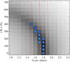 |
Fig. 9 Same as Fig. 8, but for the Fe ii 6149.3 Å line. |
| In the text | |
|
Fig. 10 Effect of Y spots on the determination of the mean longitudinal magnetic field of the HgMn star HD 11753. The curves show ⟨ Bz ⟩ as a function of rotation phase for the Y map derived by Makaganiuk et al. (2012) (thick lines) and for a uniform element distribution (thin lines). a) Calculations for the dipolar field topology with a polar strength of 500 G, obliquity β = 90°, and two different orientations with respect to the reference rotation phase (solid and dashed lines). b) Calculations for the radial magnetic field map scaled according to the Y abundance distribution. |
| In the text | |
|
Fig. 11 LSD Stokes I (left panel) and V (right panel) profiles of the HgMn star HD 11753. Thin lines show observations by Makaganiuk et al. (2012) obtained during 10 nights, starting on 2010-01-04 (top profile) and ending on 2010-01-14 (bottom profile). The thick curves correspond to the minimum-amplitude Stokes V model profiles reproducing the longitudinal field measurements obtained from the same observational data by Hubrig et al. (2012). Rotational phases are indicated on the left side of each panel. The numbers on the right side of the Stokes V panel report the probability that observations and model profiles are compatible within the error bars. |
| In the text | |
Current usage metrics show cumulative count of Article Views (full-text article views including HTML views, PDF and ePub downloads, according to the available data) and Abstracts Views on Vision4Press platform.
Data correspond to usage on the plateform after 2015. The current usage metrics is available 48-96 hours after online publication and is updated daily on week days.
Initial download of the metrics may take a while.