© ESO, 2013

1. Introduction

Recent observations with Herschel have shown the importance of filaments in star formation, as cores and clusters are embedded in or along filamentary structures (Molinari et al. 2010). In the case of massive star formation it is necessary to maintain a high gas accretion rate, and filamentary flow may be one method of achieving this (Myers 2012). Recent simulations have highlighted the importance of large scale collapse motions in forming massive star formation regions (e.g., Bonnell et al. 2006; Smith et al. 2009). In this picture, cores and clusters accrete gas from filaments that serve as mass reservoirs. Filaments may evolve from the gravitational collapse of sheets that are created by interstellar shocks, collisions of bubbles driven by supernova explosions, or stellar winds (Burkert & Hartmann 2004). Determining the velocity fields of filaments, their density, and temperature distribution are crucial to test the validity of these models. To accomplish this, large scale observations must be linked with high-spatial resolution maps on cluster scales.

The giant molecular cloud complex NGC 6334 has been explored from the radio to X-ray bands (Persi & Tapia 2010). Studies of its main ridge in the submm domain have been presented by Kraemer & Jackson (1999), Muñoz et al. (2007), Matthews et al. (2008), and Russeil et al. (2010). This region lies a bit off the Galactic plane at the Galactic coordinates l = 351.2°, b = 0.7°. The distance of (1.7 ± 0.3) kpc, determined by Russeil et al. (2012), places it in the inner edge of the Carina-Sagittarius spiral arm.

Figure 1 shows the dust continuum emission taken from APEX Telescope Large Area Survey of the Galaxy (ATLASGAL) at 870 μm/345 GHz by Schuller et al. (2009). The position angle of the filament is about PA = 35°. For practical reasons we present it here in Galactic coordinates where the filament is nearly parallel to the longitude axis. Its total length is about 12 pc, the average width (FWHM) is 0.3 pc, and the average flux is 2–3 Jy/beam and raises up to 5 Jy/beam in the vicinity of source I and I(N). The far-infrared (FIR) sources, labeled by Roman numerals in the FIR (see Kraemer & Jackson 1999), correspond to sites of massive star formation, ranging from 200–2000 M_⊙. They represent features such as H ii regions, hot molecular cores, masers, and molecular outflows. The sources are at different evolutionary stages, ranging from the cold dense core I(N) to the hot core I, and to the diffuse H ii region III in the center. This may be indicative of sequential star formation, e.g., triggered by a spiral density wave. However, other observations have revealed a more complex structure (Rodriguez et al. 1982). The gaps between the sources II and III and IV and V originate from disrupted, ionized gas of H ii regions. The white contours in Fig. 1 show the Hα emission in this region from the AAO/UKST Hα survey (Parker et al. 2005), and the position of the gaps correspond to the emission of Hα.

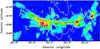Fig. 1 ATLASGAL map of NGC 6334. The continuum levels in gray are set at 0.3 (3σ), 1, 2, 5, 10, and 30 Jy/beam. The black line marks the main filament, black crosses denote FIR sources (Kraemer & Jackson 1999), and the beam width at 266 GHz is indicated in the lower-right corner. Overlaid in white contours (at 90% of the maximum intensity) is the Hα emission (Parker et al. 2005).

2. Observations and data reduction

Observations were made in July 2012 in a total time of 2 h with the 12 m single-dish submm telescope APEX to map the region displayed in Fig. 1, which has an extension of 29.4′× 13.8′. We used the APEX-2 SHeFI receiver and the XFFTS backend to measure the HCO⁺J = 3–2 (267.557 GHz) and HCN J = 3–2 (265.886 GHz) transitions. The receiver provides 32 768 channels in a bandwidth of 2.5 GHz and a maximum velocity resolution of 0.085 km s^-1. The mapped region was observed in the on-the-fly (OTF) mode with position switching and sampled with half-beam spacing and a dump time of 1 s. Pointing and focus were checked regularly on Saturn. The average value for the system temperature was 170 K and for the average precipitable water vapor 1.5 mm. The calibration uncertainty is estimated to be ~10%. The beam width (FWHM) at 267.6 GHz is θ_mb = 23.5″. The data was reduced with the GILDAS software (Pety 2005), baseline-subtracted, convolved with a Gaussian of 1/3 beam width and gridded to a map with a pixel size of θ_mb/2 = 11.75″. The spectra were converted to main-beam temperature using a main beam efficiency of η_mb = 0.75 (Wyrowski, priv. comm.) and Hanning smoothed to a velocity resolution of 0.51 km s^-1 to achieve a rms of 0.31 K.

HCO⁺ is a good tracer of dense molecular gas and well suited to examine the kinematics of infalling clumps or outflows (Rolffs et al. 2011). In order to check that the optically thick spectral lines of HCO⁺ do not consist of several, superimposed kinematic components, we compared them to complementary maps of the optically thin isotopologue H¹³CO⁺ (J = 1–0) and other molecules from the MALT90 survey (Foster et al. 2011). Only two small regions show two components in optically thin lines, the first at l = 351.42°, b = 0.66° and the second at l = 351.51°, b = 0.7°. The first one is due to the different radial velocity between source I and the filament; the second one can be explained by the superposition of multiple structures which also appear as a bifurcation in the dust emission maps of Matthews et al. (2008). Thus, the main velocity structure is not distorted by other kinematic components. In this letter, only the radial velocities of HCO⁺ are discussed without reference to local spectroscopic features of the clumps.

3. Results

3.1. Velocity field

Figure 2 shows the first moment map in HCO⁺. The highest redshifted velocity of +2 km s^-1 occurs in the center at the position of source II. There is a velocity gradient toward both ends with the highest blueshifted velocity of –7 km s^-1 at source I and V. It should be noted that the radial velocity increases again for l > 351.46°. Perpendicular to the main filament, two subfilaments exhibit longitudinal gradients at l = 351.2° and l = 351.38°. The subfilament at the position of source IV, which is tilted relative to the main filament, also shows a gradient. This was explained by Kraemer et al. (1997) as the rotation of a molecular disk around IV.

The position−velocity diagram (PVD) of NGC 6334 is presented in Fig. 3. It was created by reordering the axis from the spectral cube from xyv to xvy and by integrating over the Galactic latitude axis. The velocity gradient in the center is about 1 km s^-1 per arcmin or 2 km s^-1/pc. Small deviations from the general trend can be recognized at the position of the sources I, I(N), IV, and V. These deviations originate from outflows that cause the line profiles to have larger wings and that account for the smallest Doppler velocities below –7 km s^-1. The asymmetric double-peak profile of sources I(N) and I, apart from the filament, arises from self-absorption and infall motions and cause a slight blueshift in the radial velocity of the first moment map. The typical line width (FWHM), deduced from the N₂H⁺ and HC₃N emission lines in the MALT90 data, is δv = 1.0–2.0 km s^-1 in the filament and increases to δv = 3–4 km s^-1 in the dense clumps. These values are in agreement with the line widths reported in Russeil et al. (2010).

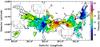Fig. 2 First moment map of the HCO+J = 3–2 transition of NGC 6334. Emission below 3σ = 0.93 K is discarded. Overlaid in black contours is the continuum emission from Fig. 1. The black arrows denote the gas flow direction.

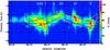Fig. 3 Position−velocity diagram of the HCO+J = 3–2 transition of NGC 6334, integrated over the Galactic latitude axis with a cutoff at 3σ = 0.93 K at each velocity channel. The position of the FIR sources are labeled above. Overlaid in contours are the PVDs of the three best-fit models of Sect. 3.3. The contours are set at 50% of the integrated emission which corresponds to the average velocity width of 3.5 km s-1 of the filament in this figure. The white contour assumes an initial velocity of zero at the edges and the red contour that the filament has already contracted from 7 to 6 pc (both at i = 45°). The model in black contours is defined with a constant velocity value of v = 10 km s-1 and i = 68°.

3.2. Analytical model

Burkert & Hartmann (2004) derive the gravitational acceleration in finite sheets and filaments. They assume a uniform, self-gravitating cylindrical cloud with a constant volume density ρ = M/(πℛ²2L), where M is the total mass, 2L is the total length, ℛ is the radius, G is the Gravitational constant, and l is the distance from the center on the longer axis. The aspect ratio is defined as A = L/ℛ. Neglecting all pressure supporting forces against the gravity (e.g., rotation, turbulence, magnetic fields), the cloud will collapse along the longer axis starting from the ends and moving toward the center. The assumption is that the radius ℛ remains relatively constant and that gravitation dominates on large (parsec) scales. The acceleration a at position l is $\mathit{a}\mathrm{\left(}\mathit{l}\mathrm{\right)}\mathrm{=}\mathrm{-}\mathrm{2}\mathit{\pi G\rho }\left[\mathrm{2}\mathit{l}\mathrm{-}\sqrt{{\mathrm{ℛ}}^{\mathrm{2}}\mathrm{+}\mathrm{(}\mathit{L}\mathrm{+}\mathit{l}{\mathrm{)}}^{\mathrm{2}}}\mathrm{+}\sqrt{{\mathrm{ℛ}}^{\mathrm{2}}\mathrm{+}\mathrm{(}\mathit{L}\mathrm{-}\mathit{l}{\mathrm{)}}^{\mathrm{2}}}\right]\mathit{.}$(1)The acceleration has the highest value at the end of the filament, which leads to a pile up and to an enhanced concentration of the gas at the periphery. In elongated elliptical sheets, the mass concentrates at the focal points. Based on this, and under the assumption that the density remains constant, Toalá et al. (2012) derive the radial velocity of the filament after it has contracted from L to l$\begin{array}{ccc}\mathit{v}\mathrm{\left(}\mathit{l}\mathrm{\right)}& \mathrm{=}& \sqrt{\mathrm{4}\mathit{\pi G\rho }}[\mathrm{(}\mathit{L}\mathrm{-}\mathit{l}\mathrm{)}\mathrm{(}\mathit{L}\mathrm{+}\mathit{l}\mathrm{+}\mathrm{ℛ}\mathrm{)}\mathrm{-}\frac{\mathit{L}}{\mathrm{2}}\sqrt{{\mathrm{ℛ}}^{\mathrm{2}}\mathrm{+}\mathrm{4}{\mathit{L}}^{\mathrm{2}}}\\ & & {\mathrm{+}\frac{\mathit{l}}{\mathrm{2}}\sqrt{{\mathrm{ℛ}}^{\mathrm{2}}\mathrm{+}\mathrm{4}{\mathit{l}}^{\mathrm{2}}}\mathrm{-}\frac{{\mathrm{ℛ}}^{\mathrm{2}}}{\mathrm{4}}\ln \left|\frac{\sqrt{{\mathrm{ℛ}}^{\mathrm{2}}\mathrm{+}\mathrm{4}{\mathit{L}}^{\mathrm{2}}}\mathrm{+}\mathrm{2}\mathit{L}}{\sqrt{{\mathrm{ℛ}}^{\mathrm{2}}\mathrm{+}\mathrm{4}{\mathit{l}}^{\mathrm{2}}}\mathrm{+}\mathrm{2}\mathit{l}}\right|]}^{\mathrm{1}\mathit{/}\mathrm{2}}\mathit{.}\end{array}$(2)The larger the aspect ratio, the smaller the rise and value of the final velocity. They also calculate the free-fall time for filaments and sheets. Whereas in the spherical case the free-fall time only depends on the density, for filaments and sheets there is an additional dependence of the geometry, characterized by the aspect ratio A. In conclusion, the free-fall time for filaments τ_ff is longer than in the spherical case τ_s, ${\mathit{\tau }}_{\mathrm{ff}}\mathrm{=}\sqrt{\frac{\mathrm{32}\mathit{A}}{\mathrm{3}{\mathit{\pi }}^{\mathrm{2}}}}\mathrm{\times }{\mathit{\tau }}_{\mathrm{s}}\mathrm{=}\sqrt{\frac{\mathrm{32}\mathit{A}}{\mathrm{3}{\mathit{\pi }}^{\mathrm{2}}}}\mathrm{\times }\sqrt{\frac{\mathrm{3}\mathit{\pi }}{\mathrm{32}\mathit{G\rho }}}\mathrm{·}$(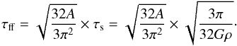3)

3.3. Application to NGC 6334

We aim to take the velocities predicted from Eq. (2) and to compare them with the observations of NGC 6334. Although Eq. (2) is not applicable for every position l of the filament at one point in time, it is a good approximation for cases with high aspect ratios where the value of the radial velocity increases only slightly during the collapse. Furthermore, we consider only the longitudinal velocity and assume that the radius ℛ stays constant. As the shape of the filament is not a regular cylinder but is curved elliptically, a generalized conic section is used via the implicit function $\sqrt{{\mathit{x}}^{\mathrm{2}}\mathrm{+}{\mathit{y}}^{\mathrm{2}}}\mathrm{=}\mathrm{(}\mathit{l}\mathrm{+}\mathit{e}\mathrm{\ast }\mathit{x}\mathrm{)}\mathit{,}$(4)where l is the semi-latus rectum and e the eccentricity. The latus rectum is the line segment through the focus and is perpendicular to the major axis a. The eccentricity of an ellipse is defined as $\mathit{e}\mathrm{=}\sqrt{\mathrm{1}\mathrm{-}\mathrm{(}\mathit{b}\mathit{/}\mathit{a}{\mathrm{)}}^{\mathrm{2}}}$, where b is the minor axis. We assume that the direction of the velocity v is determined by the shape of the filament. Then the velocity direction field is gained from the derivative of Eq. 4 and normalized to unit vectors $\begin{array}{ccc}{v}\mathrm{=}\mathrm{(}\mathit{x,}\mathit{y}\mathrm{)}\mathrm{=}& & \\ \left(\frac{\mathit{y}}{\sqrt{{\mathit{y}}^{\mathrm{2}}\mathrm{+}\mathrm{\left(}\mathrm{\right(}\mathit{l}\mathrm{+}\mathit{e}\mathrm{\ast }\mathit{x}\mathrm{)}\mathrm{\ast }\mathit{e}\mathrm{-}\mathit{x}{\mathrm{)}}^{\mathrm{2}}}}\mathit{,}\frac{\mathrm{(}\mathit{l}\mathrm{+}\mathit{e}\mathrm{\ast }\mathit{x}\mathrm{)}\mathrm{\ast }\mathit{e}\mathrm{-}\mathit{x}}{\sqrt{{\mathit{y}}^{\mathrm{2}}\mathrm{+}\mathrm{\left(}\mathrm{\right(}\mathit{l}\mathrm{+}\mathit{e}\mathrm{\ast }\mathit{x}\mathrm{)}\mathrm{\ast }\mathit{e}\mathrm{-}\mathit{x}{\mathrm{)}}^{\mathrm{2}}}}\right)\mathrm{·}& & \end{array}$(5)The total mass of NGC 6334 within the observed region is estimated to be M = 16   700–23   100 M_⊙ (Matthews et al. 2008; Muñoz et al. 2007), where half of this is contained in the seven most massive clumps. Eliminating I, I(N), and the other sources that do not lie on the filament and given the uncertainties, it is assumed that the ridge mass is M ≈ 10⁴M_⊙. A slightly larger radius of ℛ = 0.2 pc is adopted for the analytical model because the observed density profile follows a Plummer-like function and does not vanish at the observed radius of 0.15 pc. Matthews et al. (2008) derive average dust temperatures of 25 K and higher average gas temperatures of 50 K in the filament. The average hydrogen column density is N_H2 = 5 × 10²² cm^-3 (Matthews et al. 2008), resulting in a density of n_H2 = 5 × 10⁴ cm^-3. Using the density formula in Sect. 3.2, the analytical model has an average density of n = 1 × 10⁵ cm^-3, twice as large as the observed density because the massive clumps are included. The value of v obtained from Eq. (2) is then about 10–20 km s^-1.

Using the geometry and analytical velocity field above, we create a model of the filament with the 3D radiative transfer code LIME (Brinch & Hogerheijde 2010) and produce synthetic HCO⁺ (J = 3–2) observations. The parameters in the LIME code match the values of NGC 6334, with a constant gas temperature of 50 K, a constant density of n = 5 ×10⁴ cm^-3, a radius of 0.2 pc, a line width of 1.7 km s^-1, and a fractional abundance of X(HCO⁺) = 2 × 10^-9. The HCO⁺ abundance in NGC 6334 lies in the range of 5 × 10^-10 to 5 × 10^-9, which is found in other star-forming regions (Godard et al. 2010). The resulting spectral cubes are convolved with the APEX beam width, rotated by the angle PA and i, where PA is the fixed position angle and i the inclination, and the same reduction steps are applied as for the data to obtain the PVD. An inclination of 0° corresponds to a face-on view. Because the radial velocity is nonzero along the line of sight, it is clear that i > 0°. A parameter study of the free parameters e and i shows that small eccentricities are a poor match to Figs. 1 and 3. Consequently, if this model is true the filament cannot be circular. On the other hand, values of e > 1.5 result in a straight shape. The values that best fit both the dust continuum map and the PVD are e ≈ 0.9 and i ≈ 45° (see the contours in Fig. 3). The white model corresponds to the actual observed size with a half-length of L = 6 pc. The red model presumes that the initial conditions were L = 7 pc, so that the filament has contracted by 1 pc at the edges, which would take a time of 4 × 10⁵ yr. The black model assumes a constant velocity value of v = 10 km s^-1 throughout the cylinder and a higher inclination of i = 68°. The red model shows the best fit to the data. The white model underestimates the radial velocity at the edges, meaning that the observed filament must have been already contracted. On the other hand, the black model overpredicts the radial velocity at the edges, illustrating that the velocity magnitude is not constant.

4. Discussion

A PVD of NGC 6334 was presented by Batchelor et al. (1984) in HCO⁺ 1–0 and by Kraemer & Jackson (1999) from CS and CO observations. Both analyses suggested a collapse or an expansion. Based on the FIR sources which lie mostly on the major axis of this elliptical cloud, Dickel et al. (1977) presented a spherical model of a global collapse. The new observations reveal the filamentary and subfilamentary structure in dust and molecular emission and a coherent velocity field. The symmetric shape in Fig. 3, and the fact that the highest blueshifted emission stems from the region with the highest density (1.7 × 10⁵ cm^-3 in source V and 1.2 × 10⁶ cm^-3 in source I, Russeil et al. 2010), agrees with the predictions in Sect. 3.2, where the gas accumulates at the filament’s edges. The emission at l > 351.46° that causes the slightly unsymmetrical shape in Fig. 3 can be explained by later infall from ambient gas and the presence of multiple components as mentioned in Sect. 2. We note the fact that the dense region at source I and I(N) formed out of the major axis is a deviation to the idealized model of Sect. 3.2. This deviation could be explained by a non-uniform density distribution and cloud geometry at the beginning of the collapse, as is shown by Burkert & Hartmann (2004) for irregular cloud boundaries. The HCN spectra indicate that this region is collapsing and thus may have decoupled from the rest of the filament.

There are two other possible explanations for the velocity field. First, the whole filament could be collapsing toward a focal point above the filament’s center away from the observer (see e.g., Burkert & Hartmann 2004, Fig. 11). However, this would lead to the highest densities in the center, as opposed to the observations. Moreover a gravitational focal center could not be assigned to any visible source. Secondly, there is an uncertainty about the direction of the velocity when a gradient is observed. Excluding rotational effects, one expects the flow to be toward the largest center of mass. As the sources I, I(N), and IV have the highest mass, this could mean that the central part of the filament is moving toward it. The observed high stellar activity in this region has already disrupted some of the gas and may be complicating the gas motions. Bright sources could even reverse the velocity gradients. However, an expansion motion, caused by stellar winds or shocks, would need strong excitation sources near the center of the filament, but the stellar clusters and OB stars are inhomogeneously distributed throughout (Feigelson et al. 2009). In conclusion, while the local gas motions may be affected by feedback, the global velocity structure over 12 pc suggests a large-scale collapse scenario.

The observed aspect ratio of NGC 6334 is A = 6 pc/0.15 pc = 40. From Eq. (3) and using a mean density of n = 5 × 10⁴ cm^-3, we derive a free-fall time of τ_ff = 1.0 Myr. As we have not

considered any additional supportive forces, this value should be taken as a lower limit. The resulting free-fall time is one magnitude longer than the lifetimes of massive protostars in NGC 6334 of 10⁴–10⁵ yr (Russeil et al. 2010), which means that these protostars may evolve while the filament is contracting. We used the constant density approach of Toalá et al. (2012), but they also discuss another approach where the total mass is conserved and ρ is variable. This second approach overestimates the gravitational attraction during the collapse, and it is estimated that the actual timescale lies between these two cases. While Toalá et al. (2012) are sensitive to the collapse dynamics at the edge of a cylinder, Pon et al. (2012) probe the timescale of the interior of a cylinder and find a linear dependence of the free-fall time on A, τ ~ 0.82Aτ_s. This homologous collapse assumes that the total mass is conserved and would result in τ = 5.0 Myr for NGC 6334. However, the edge-driven collapse (Sect. 3.2) becomes more dominant than the homologous collapse in elongated filaments with large aspect ratios (A ≫ 1). As this is the case in NGC 6334, the edge-driven scenario with a lower free-fall time of 1 Myr will be more likely.

In summary, we have presented APEX observations in HCO⁺ of the main filament in NGC 6334. The radial velocities indicate a global gravitational collapse in agreement with theoretical models. After the determination of the global velocity field, the next step is to look for the local structure in the clumps and possible infall motions. For source I and I(N), high-resolution interferometric data from the Submillimeter Array is available at 355 GHz, including the HCN/HCO⁺J = 4–3 transition and its isotopologues. This will allow us to trace the gas flow motions in the fragmented clumps to scales of 1″ or 1700 AU.

Acknowledgments

This work was carried out within the Collaborative Research Council 956 and 881, funded by the Deutsche Forschungsgemeinschaft (DFG). R. Smith acknowledges support for grant No. SM321/1-1 from the DFG Priority Program 1573. We thank F. Wyrowski and the APEX staff for carrying out the observations.

References

All Figures

	Fig. 1 ATLASGAL map of NGC 6334. The continuum levels in gray are set at 0.3 (3σ), 1, 2, 5, 10, and 30 Jy/beam. The black line marks the main filament, black crosses denote FIR sources (Kraemer & Jackson 1999), and the beam width at 266 GHz is indicated in the lower-right corner. Overlaid in white contours (at 90% of the maximum intensity) is the Hα emission (Parker et al. 2005).
In the text

	Fig. 2 First moment map of the HCO+J = 3–2 transition of NGC 6334. Emission below 3σ = 0.93 K is discarded. Overlaid in black contours is the continuum emission from Fig. 1. The black arrows denote the gas flow direction.
In the text

Fig. 3 Position−velocity diagram of the HCO+J = 3–2 transition of NGC 6334, integrated over the Galactic latitude axis with a cutoff at 3σ = 0.93 K at each velocity channel. The position of the FIR sources are labeled above. Overlaid in contours are the PVDs of the three best-fit models of Sect. 3.3. The contours are set at 50% of the integrated emission which corresponds to the average velocity width of 3.5 km s-1 of the filament in this figure. The white contour assumes an initial velocity of zero at the edges and the red contour that the filament has already contracted from 7 to 6 pc (both at i = 45°). The model in black contours is defined with a constant velocity value of v = 10 km s-1 and i = 68°.

In the text

References

- Batchelor, R. A., Robinson, B. J., & McCulloch, M. G. 1984, PASA, 5, 363 [NASA ADS] [Google Scholar]
- Bonnell, I. A., Dobbs, C. L., Robitaille, T. P., et al. 2006, MNRAS, 365, 37 [NASA ADS] [CrossRef] [Google Scholar]
- Brinch, C., & Hogerheijde, M. R. 2010, A&A, 523, A25 [NASA ADS] [CrossRef] [EDP Sciences] [Google Scholar]
- Burkert, A., & Hartmann, L. 2004, ApJ, 616, 288 [NASA ADS] [CrossRef] [Google Scholar]
- Dickel, H. R., Dickel, J. R., & Wilson, W. J. 1977, ApJ, 217, 56 [NASA ADS] [CrossRef] [Google Scholar]
- Feigelson, E. D., Martin, A. L., McNeill, C. J., et al. 2009, AJ, 138, 227 [NASA ADS] [CrossRef] [Google Scholar]
- Foster, J. B., Jackson, J. M., Barnes, P. J., et al. 2011, ApJS, 197, 25 [NASA ADS] [CrossRef] [Google Scholar]
- Godard, B., Falgarone, E., Gerin, M., et al. 2010, A&A, 520, A20 [NASA ADS] [CrossRef] [EDP Sciences] [Google Scholar]
- Kraemer, K. E., & Jackson, J. M. 1999, ApJS, 124, 439 [NASA ADS] [CrossRef] [Google Scholar]
- Kraemer, K. E., Jackson, J. M., Paglione, T. A. D., et al. 1997, ApJ, 478, 614 [NASA ADS] [CrossRef] [Google Scholar]
- Matthews, H. E., McCutcheon, W. H., Kirk, H., et al. 2008, AJ, 136, 2083 [NASA ADS] [CrossRef] [Google Scholar]
- Molinari, S., Swinyard, B., Bally, J., et al. 2010, A&A, 518, L100 [NASA ADS] [CrossRef] [EDP Sciences] [Google Scholar]
- Muñoz, D. J., Mardones, D., Garay, G., et al. 2007, ApJ, 668, 906 [NASA ADS] [CrossRef] [Google Scholar]
- Myers, P. C. 2012, ApJ, 752, 9 [NASA ADS] [CrossRef] [Google Scholar]
- Parker, Q. A., Phillipps, S., Pierce, M. J., et al. 2005, MNRAS, 362, 689 [NASA ADS] [CrossRef] [Google Scholar]
- Persi, P., & Tapia, M. 2010, Mem. Soc. Astron. Italiana, 81, 171 [Google Scholar]
- Pety, J. 2005, in SF2A-2005: Semaine de l’Astrophysique Francaise, eds. F. Casoli, T. Contini, J. M. Hameury, & L. Pagani, 721 [Google Scholar]
- Pon, A., Toalá, J. A., Johnstone, D., et al. 2012, ApJ, 756, 145 [NASA ADS] [CrossRef] [Google Scholar]
- Rodriguez, L. F., Canto, J., & Moran, J. M. 1982, ApJ, 255, 103 [NASA ADS] [CrossRef] [Google Scholar]
- Rolffs, R., Schilke, P., Wyrowski, F., et al. 2011, A&A, 527, A68 [NASA ADS] [CrossRef] [EDP Sciences] [Google Scholar]
- Russeil, D., Zavagno, A., Motte, F., et al. 2010, A&A, 515, A55 [NASA ADS] [CrossRef] [EDP Sciences] [Google Scholar]
- Russeil, D., Zavagno, A., Adami, C., et al. 2012, A&A, 538, A142 [NASA ADS] [CrossRef] [EDP Sciences] [Google Scholar]
- Schuller, F., Menten, K. M., Contreras, Y., et al. 2009, A&A, 504, 415 [NASA ADS] [CrossRef] [EDP Sciences] [Google Scholar]
- Smith, R. J., Longmore, S., & Bonnell, I. 2009, MNRAS, 400, 1775 [NASA ADS] [CrossRef] [Google Scholar]
- Toalá, J. A., Vázquez-Semadeni, E., & Gómez, G. C. 2012, ApJ, 744, 190 [NASA ADS] [CrossRef] [Google Scholar]