| Issue |
A&A
Volume 554, June 2013
|
|
|---|---|---|
| Article Number | A75 | |
| Number of page(s) | 9 | |
| Section | Extragalactic astronomy | |
| DOI | https://doi.org/10.1051/0004-6361/201220631 | |
| Published online | 06 June 2013 | |
Evidence for a cosmological effect in γ-ray spectra of BL Lacertae ⋆
1 Max-Planck-Institut für Kernphysik, PO Box 103980, 69029 Heidelberg, Germany
e-mail: This email address is being protected from spambots. You need JavaScript enabled to view it.
2 Laboratoire Leprince-Ringuet, Ecole polytechnique, CNRS/IN2P3, 91128 Palaiseau, France
Received: 25 October 2012
Accepted: 22 March 2013
Abstract
We update the list of GeV-TeV extragalactic γ-ray sources using the two-year catalog from the Fermi Large-Area Telescope (LAT) and recent results from ground-based γ-ray telescopes. Breaks in the spectra between the high-energy (100 MeV < E < 300 GeV) and the very high-energy (E > 200 GeV) ranges, as well as their dependence on distance, are discussed in the context of absorption on the extragalactic background light (EBL). We calculate the size of the expected break using a model for the EBL and compare it to the data, taking into account systematic uncertainties in the measurements. We develop a novel Bayesian model to describe this dataset and use it to constrain two simple models for the EBL-induced breaks.
Key words: BL Lacertae objects: general / cosmic background radiation / gamma rays: galaxies
Appendices are available in electronic form at http://www.aanda.org
© ESO, 2013
1. Introduction
The extragalactic background light (EBL) is a diffuse field of UV, optical, and infrared photons, with wavelengths in the range λ = 0.1 − 1000 μm, on which the integrated history of star formation in the Universe is imprinted. The spectral energy distribution (SED) of the EBL consists of two distinct components: the first, peaking in νFν around ≃ 1 μm and commonly referred to as the cosmic optical background (COB), was produced by thermal emission from stars since the big bang. The second component peaks at longer wavelengths (≃100 μm), has peak energy density comparable to the COB. It is referred to as the cosmic infrared background (CIB), and originates from the absorption and reemission of starlight by dust (see Hauser & Dwek 2001, for review).
Direct measurements of the EBL density are difficult due to local foregrounds, such as the zodiacal light and Galactic radiation (Hauser & Dwek 2001). They and are often interpreted as upper limits, while galaxy number counts in optical or infrared provide lower limits (Madau & Pozzetti 2000).
Since γ rays of observed energy Eγ can interact with EBL photons of energy EEBL at a redshift z through γγ → e+ + e− when Eγ/1 TeV > 0.26 eV/EEBL(1 + z), the spectra of distant extragalactic sources measured in the very high-energy (VHE, E > 200 GeV) regime should differ from their emitted (intrinsic) spectra if the EBL density is nonzero1. Since a large fraction of the emitted power in BL Lac-type blazars is in γ-ray band, this must be accounted for when SEDs are used to model their underlying physical properties (Coppi & Aharonian 1999).
Finding clear evidence for this EBL-induced attenuation has proven remarkably difficult to date. The fall-off in the EBL spectral density between the COB and CIB peaks (around 0.1 eV) should be visible as a kink in the measured VHE spectra around 1 TeV. This was sought, for example, in the blazar H 1426+428 by Aharonian et al. (2003), but results have been inconclusive given the large statistical errors. The signature of the EBL should also be evident in studies of the global population of VHE sources. This is because the energy-dependent attenuation increases with distance, such that the observed spectra are expected to become softer, i.e., the photon index, Γ, in power-law spectral fits should increase with redshift, z. Such studies have not been successful, with no evidence for a redshift-dependent effect being found by Mori (2009), De Angelis et al. (2009, the authors attributing this to varying spectral states inducing a large scatter in the data), or Orr et al. (2011, see in particular Fig. 13).
It has, however, been possible to constrain the EBL density in the energy range where they interact with observed γ rays. Using VHE spectra from distant BL Lac objects and a theoretically motivated conjecture that the photon index of the intrinsic spectrum cannot be harder than ΓI ≃ 1.5, several authors have derived upper limits for the density close to the lower limits from galaxy counts (Dwek & Krennrich 2005; Aharonian et al. 2006). Recently, Ackermann et al. (2012) and Abramowski et al. (2013) measured the EBL density using its imprint in the spectra of BL Lac objects and found a density of EBL compatible with the best upper limits to date (Meyer et al. 2012).
Operating as an all-sky monitor, the Fermi LAT (Atwood et al. 2009) observes γ rays in the high energy (HE, 100 MeV < E < 300 GeV) range, where the effects of the EBL are much smaller than in the VHE. Sources detected both in the HE by Fermi and in the VHE by imaging atmospheric-Cherenkov telescopes (IACTs) then provide an opportunity to probe the effects of the energy-dependent attenuation from the EBL absorption across a much wider energy range. Here we present an updated list of GeV-TeV sources, building on the work of Abdo et al. (2009) and Ackermann et al. (2011).
2. Selection of the sources
Since the first detection of an extragalactic γ-ray source in the VHE range by Whipple (Punch et al. 1992), 50 active galactic nuclei (AGN) have been discovered in this energy band. The rate of detections has increased dramatically with the increased sensitivity of the latest generation of IACTs (VERITAS, MAGIC and H.E.S.S.) and an improved observation strategy using data from the Fermi LAT. An up-to-date view of the VHE sky can be found by browsing the TeVCat catalog2 (Wakely & Horan 2008).
We selected AGN from TeVCat for which an HE and a VHE spectrum have been published and a firm redshift determined. Of the 50 AGN, 30 are BL Lacs with published spectral information. Three of these, namely, 3C 66A, PKS 1424+240, and PG 1553+113, do not have a firm redshift determination. In addition, there are two VHE-detected flat-spectrum radio quasars (FSRQs), 3C 279 and 4C +21.35. Despite their large redshift (see Table 1), internal absorption close to the emission region may strongly affect their spectra (Aharonian et al. 2008; Sitarek & Bednarek 2008); hence we include them in this study only for illustrative purposes. We also include the radio galaxies Centaurus A and M 87 in the sample.
The second Fermi catalog of AGN (2LAC, Ackermann et al. 2011) includes 1057 sources associated with AGN of many kinds. In this list, 36 out of the 37 VHE BL Lacs have a Fermi counterpart; the six that are not detected are SHBL J001355.9-185406, 1ES 0229+200, 1ES 0347-121, PKS 0548-322, HESS J1943+213, and 1ES 1312-423.
List of HE-VHE BL Lacs and radio galaxies. Only statistical errors are given.
By merging the two lists, our sample contains 23 HE-VHE BL Lacs and two radio galaxies. The characteristics of these sources are listed in Table 1, including the photon indexes from published power-law spectral fits in the HE (from 2LAC) and VHE (from the reference given in the table), which form the dataset for this study.
AGN are observed to be variable in all wavelengths. In the VHE regime, flaring episodes have been observed from a number of such sources, in particular those that are bright and/or close by (such as Mrk 421, Mrk 501, and PKS 2155−304). However, most have not shown clear evidence of variability, many having been detected close to the sensitivity threshold of the instrument. It is not improbable that variability is a common feature of HBLs in the VHE regime, future instruments will be able to probe this in a larger population of fainter, more distant sources. In the HE range, BL Lacs, and especially high-frequency peaked BL Lacs (HBLs), are found to be the less variable (Abdo et al. 2010a). To reduce any bias introduced by the use of non-simultaneous observations, we used the VHE spectrum that has the lowest flux reported in the literature, which results in a generally good agreement between the overlapping energy ranges (Abdo et al. 2009).
3. Interpretation
3.1. Spectral evolution with the redshift
The mean HE and VHE indexes of our sample are ⟨ ΓHE ⟩ = 1.86 and ⟨ ΓVHE ⟩ = 3.18, respectively. For each source the photon index measured in the VHE range is greater than or compatible with that found in the HE, i.e., ΔΓ = ΓVHE − ΓHE ≳ 0. In the HE band, the standard deviation of the measured indexes is σHE = 0.26, and the excess variance, which accounts for the measurement errors3, is  . In the VHE regime, the standard deviation is σVHE = 0.49, while the excess variance is
  , showing that most of the sample variance can be ascribed to the errors on the individual measurements rather than to the intrinic distribution.
The points in Fig. 1 show ΔΓ versus the redshift z for our sample of sources. The two close-by radio galaxies do not show significant spectral breaks. For all other sources, ΔΓ ≳ 0.5, and those more distant than z = 0.1 exhibit a break of ΔΓ ≳ 1.0. A dependence of ΔΓ with z is apparent in our sample.
If we were to assume that the intrinsic spectrum of each object was well represented by a single power law across the entire HE and VHE domain, as seems to be the case for the two nearby radio galaxies for which ΔΓ ~ 0, we should expect that any significant break in the measured spectrum is the result of absorption on the EBL, i.e.,  , where τ(Eγ,z) is the optical depth due to the attenuation by pair production (Abdo et al. 2009, Eq. (2)). To leading order, the EBL break increases linearly with the redshift, and we would expect ΔΓ to be correlated with z. The Pearson correlation factor for our dataset is ρ = 0.56 ± 0.11, more than 5σ away from 0, showing clear evidence that this dependency exists.
In Appendix B.2 we outline a simple method to evaluate the size of the break that might be expected from redshifting a curved intrinsic synchrotron self-Compton (SSC) spectrum within the HE and VHE observation windows, which gives rise to a K correction for the measured spectral indexes. This study shows that such a K correction would account for ~15% of the observed break for the most distant source in the sample at z = 0.3.
3.2. Expected EBL-induced spectral break
To further evaluate the data, we estimated the size of the spectral break as a function of redshift from the EBL density model of Franceschini et al. (2008, hereafter Fra08). We performed a simple simulation in which a hypothetical source with a flat spectrum (ΓI = 0) is placed at a distance z and its flux attenuated by the EBL. The spectrum is simulated in 20 logarithmically spaced bins per decade. To evaluate the measured index a power law model if fitted to the bins above 200 GeV, with equal weighting per bin. The limited photon flux at the highest energies is accounted for in an ad hoc manner; the upper energy bound of the fit is chosen to be the point at which the differential flux is 1% of the flux at 200 GeV (up to a maximum of 10 TeV).
The predicted ΔΓ(z) is the black line shown in Fig. 1. The shaded gray areas show uncertainties on this calculation, which arise from:
-
the ~10% energy resolution typical of IACTs, which is taken into account by shifting the energy bins by ± 10% (dark gray area),
-
the threshold energy of the observations, which can vary from 100 GeV to more than 500 GeV (gray area), and
-
the systematic error on the measured photon spectral index, typically 0.2 (light gray).
It is clear from Fig. 1 that, for the majority of sources, the observed break, ΔΓ, is systematically larger than that predicted by the EBL model, ΔΓEBL. This is most notably the case for 1ES 2344+514 (z = 0.044), PKS 2005-489 (z = 0.071), W Comae (z = 0.102), PKS 2155-304 (z = 0.116), and H 1426+428 (z = 0.129). The difference, ΔΓ − ΔΓEBL, is almost certainly the result of (convex) intrinsic curvature in the spectra of these objects, which is not unexpected (Perlman et al. 2005) and can have several interpretations, for instance, as being due to a turnover in the distribution of the underlying emitting particles (acceleration effects; e.g., Massaro et al. 2006) or to Klein-Nishina suppression (emission effects).
Nevertheless, it is striking that there are many sources for which ΔΓ ≃ ΔΓEBL. For these sources, the intrinsic broad-band γ-ray spectra are compatible (within errors) with single power laws. For those that additionally have ΓHE ≲ 2.0, the high-energy peaks are not constrained by the current observations, even though they have a well-defined observational νFν peak. The most striking examples are H 2356-309 (z = 0.129), 1RXS J101015.9-311909 (z = 0.142), 1ES 1101-232 (z = 0.186), 1ES 0414+009 (z = 0.287), and S5 0716+714 (z = 0.310).
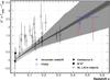 |
Fig. 1 Value of ΔΓ as a function of the redshift z. The black line is the theoretical break obtained with the Franceschini et al. (2008) model. The uncertainties due to the energy resolution of IACTs (dark gray), the different threshold energies (medium gray), and the systematic errors of 0.2 (light gray) are shown. The FSRQs and the BL Lacs with uncertain redshift are shown for illustration. |
Summary of results with the linear parametrization and scaled Franceschini et al. (2008) EBL model obtained with the Bayesian approach described in the text.
3.3. Constraining the EBL density
Since a significant fraction of the observed break can be directly attributed to the EBL, we attempted to constrain its density by applying a Bayesian model, which takes into account the effects discussed in the previous section. The model is described fully in Appendix A. We used two prescriptions to account for the effects of the EBL on the spectra, ΔΓEBL(E,z). In the first, the break is modeled as a linear function of the redshift, with coefficient a (as in Stecker & Scully 2006). We further assumed that the VHE measurements cover approximately the same energy range, so that the effect of energy threshold can be neglected:  (1)In the second model we applied a scaling factor, α, to the EBL model of Fra08, which resulted in an expected break of
  (2)where ΔΓFra08(Ei,zi), was calculated for each source as in Sect. 3.2.
For both models, the posterior probability is computed and the results are given in Table 2. Figure 2 depicts the resulting ΔΓ for each model, using the mean value (i.e., ⟨ a ⟩ and ⟨ α ⟩) and the 95% confidence level (CL) lower limit (i.e., aP < 95% and αP < 95%).
The Bayesian model gives a value of ⟨ a ⟩ = 5.37 ± 0.65 and a 95% CL upper limit of 6.44 for the linear EBL model, which is significantly less than the value of 8.4 ± 1.0 reported by Yang & Wang (2010) using a simple χ2 fit, which did not account for the intrinsic breaks. Stecker & Scully (2010) found that their baseline model can be approximated by a linear coefficient of 7.99, which cannot be reconciled with the results presented here. The null hypothesis, i.e., that there is no dependence of ΔΓ with the redshift (a = 0), is rejected at more than 8σ. The spectral break predicted using the model of Fra08 is in good agreement with the data; the mean scaling factor is ⟨ α ⟩ = 0.85 ± 0.10 and the 95% CL limit is α < 1.02.
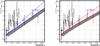 |
Fig. 2 Value of ΔΓ as a function of the redshift z. Overlaid are the predicted breaks obtained from the Bayesian fit (simple line), as well as the 95% CL lower limits (hashed area). Left is the linear approximation (Eq. (1)) and right is the scaled model of Fra08 (Eq. (2)). For both models, none of the sources are significantly lower than the 95% CL lower limit. The symbols are descibed in Fig. 1. |
4. Conclusions and perspectives
We have shown that broad-band γ-ray spectra (from ~ 100 MeV to a few TeV) carry the imprint of the EBL and provide a unique dataset to probe its properties. The redshift dependence of the difference of the photon indexes in VHE and HE range, ΔΓ, is found to be compatible with expectations from EBL attenuation. The Pearson correlation coefficient shows that ΔΓ and z are significantly correlated. We developed a Bayesian model to fit the dataset, accounting for intrinsic spectral softening, and find that the EBL density is consistent with the value predicted by Franceschini et al. (2008). Similar results have been found by Ackermann et al. (2012) and Abramowski et al. (2013), who modeled the EBL-absorbed spectra of AGNs detected in the HE and VHE regimes and found scaling factors of αFermi = 1.02 ± 0.23 and  , respectively. Their approach has the potential to be more powerful than that used here, since it can probe the features of the EBL-absorption signature as a function of energy. However, their approach is more reliant on the detailed modeling of the intrinsic spectra of the objects and of the EBL density and does not take advantage of the wider energy band available when the HE and VHE observations are combined. The two approaches are complementary and yield roughly compatible results within the combined statistical and systematic errors. Taking only the statistical errors, a χ2 fit to the HESS, Fermi, and our results gives a mean value of αcombined ≈ 0.98 and a value of χ2 = 5.45 for two degrees of freedom, compatible with the hypothesis that the values are consistent at the 1.85σ level. Our model also offers a simple prescription for constraining the redshift of a GeV-TeV sources based on their measured value of ΔΓ (see Appendix A). Applying our findings to PG 1553+113 and 3C 66A leads to z < 0.64 and z < 0.55, respectively, in good agreement with the spectroscopic constraints.
No sources have breaks significantly smaller than ΔΓEBL. Significant deviations from the expected EBL-induced spectral breaks could indicate either that there is concave curvature in the intrinsic spectrum of the source or that other processes are at play during the propagation of γ rays, such as cosmic-ray interactions along the line of sight, which create spectral softening in high-redshift source spectra (Essey & Kusenko 2012). Our findings indicate that experimental uncertainties need to improve and firmer redshift estimations be established before the significance of this effect can be assessed.
The recent commissioning of the 28 m H.E.S.S. 2 telescope, the commissioning of the upgraded MAGIC telescopes, and the upgrade of the VERITAS cameras and trigger should increase the distance at which new blazars can be detected, while the planned CTA project (Actis et al. 2011) should reduce the uncertainties mentioned above due to its superior sensitivity. Finally, a useful feature of studies of spectral breaks vs. redshift, such as this one, is their capacity to provide distance estimations for BL Lacs (see, e.g., Abdo et al. 2010b; Prandini et al. 2010, 2012), since an estimated 50% of this population has an unknown or uncertain redshift.
Online material
Appendix A: Bayesian model
Appendix A.1: Development of the model
To extract information about the EBL density from the data presented in Fig. 1, we develop a “hierarchical” Bayesian model (using the terminology of Gelman et al. 2003), which is described by source-by-source spectral parameters and global parameters specifying, among other things, the EBL density of primary interest here. We use a Bayesian methodology to write the posterior density for the model parameters, marginalize over the source-by-source parameters that are not of interest, and produce estimates and confidence intervals for the EBL density.
In the development below, we make repeated use of the conditional probability rule (CPR) that the joint probability of two (sets of) events A and B, P(A,B), can be expressed as P(A,B) = P(A | B)P(B). If the two events are independent this becomes P(A,B) = P(A)P(B). We also frequently use the rule for marginalizing (or integrating) over unwanted parameters, P(A) = ∫P(A,B)dB. Finally, we use the standard identity for the product of two Gaussians (see, e.g., Ahrendt 2005). In particular, if N(x | μ,σ2) denotes a Gaussian distribution with mean μ and variance σ2, then  (A.1)The dataset to be modeled consists of N GeV and TeV spectral measurements,
  and
and  with measurement variances of
  and
and  and redshifts zi (which are themselves not considered as measurement data). In what follows we refer frequently to the measured spectral break,
  . We write the dataset as
  .
.
Each source is parametrized by four values, the intrinsic spectral indexes in the GeV and TeV regimes,  and
and  , and the spectral indexes after absorption by the EBL,
  and
and  . In what follows we refer frequently to the intrinsic spectral break,
  . The global parameters that describe the EBL absorption itself are denoted abstractly as G and we write the set of all parameters of the model as
  .
.
Bayes’ theorem allows us to write the posterior probability distribution of the parameters after the measurements have been made, P(Θ | Y), in terms of the standard likelihood of the data, P(Y | Θ), and the prior probability distribution of the model parameters, P(Θ): 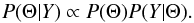 The relation is written as a proportionality, instead of as an equality, because a global normalization factor has been neglected.
The model has four primary components that we discuss below. These are: (1) the likelihood for the GeV and TeV measurements, given the true absorbed spectral indexes of the sources; (2) a relationship between the absorbed index in the GeV regime and the intrinsic (unabsorbed) index; (3) a relationship for the analogous indexes in the TeV regime; and (4) a specification of how the intrinsic index in the GeV regime is related to the intrinsic index in the TeV regime.
We assume that the measurements of the individual indexes are independent (no correlation between measurements from different sources or between the GeV and TeV bands) and that the distribution for each measurement ( or ) is Gaussian with mean given by the appropriate absorbed index and with variance given by the measurement errors squared. Therefore, the likelihood is 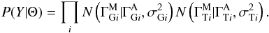 For the prior, we assume that the only link between the source-by-source index parameters for different sources comes through the global parameters G. Therefore, using the CPR we can write
 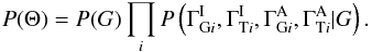 It now remains only to describe how the intrinsic and absorbed indexes for each source are related. We assume that the absorbed index in each band depends only on the intrinsic index in that band and on the EBL parameters. Repeatedly applying the CPR, this gives
 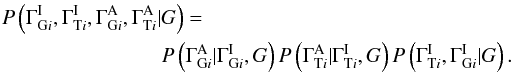 (A.2)We further assume that there is no absorption in the GeV regime and that the absorption in the TeV regime changes the index in a deterministic way. Specifically, we assume that (i)
  , and (ii)
  , where ΔΓEBL(Ei,zi | G) is a function giving the change in TeV index for a source at redshift zi measured at a TeV “threshold” energy of Ei. This can be expressed in terms of a probability using the Dirac δ-function:
 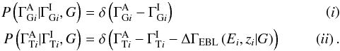 Equation (A.2) then reads
 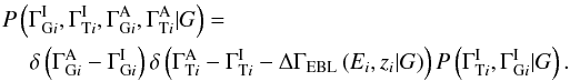 The final and most interesting part of the model is to describe how the intrinsic indexes in the two bands are related. We expand this using the CPR to give
 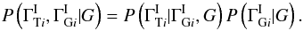 We adopt a uniform prior for ,
  and restrict ourselves to forms for the conditional probability that can be expressed as a function of the intrinsic break,
 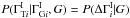 . We assume that the break for each source is drawn from a single universal distribution that has, at most, some dependence on the global parameter set, G. The final expression for the prior for the parameters of each source is
 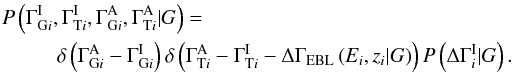 Putting everything together, recognizing that we have not yet discussed the parameters G, and leaving the exact choice of prior for the intrinsic break open for the present time, the full posterior density is
 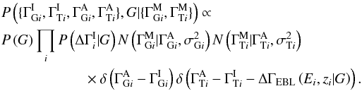 We marginalize over the parameters that are not of interest, , , , and to give the posterior probability for the global parameters G. The integrals over the parameters for each source can be done separately:
 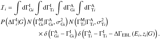 The integrals over and can be done immediately against the delta functions to give
 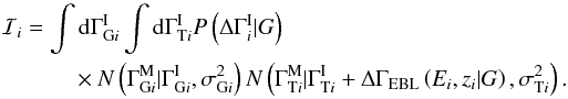 Making a change of integration variable from to
  , the Gaussians can be manipulated to give
 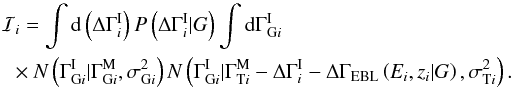 The second integral can be evaluated using Eq. (A.1). Putting all the source integrals together gives the general expression
 ![Mathematical equation: \appendix \setcounter{section}{1} \begin{eqnarray} \label{EQ::POSTERIOR_DGAMMA_GENERAL} P\left(G|\{\Gamma_{\mathrm{G}i}^{\rm M}, \Gamma_{\mathrm{T}i}^{\rm M}\}\right) \propto P\left(G\right)\nonumber\\ \prod_i \int {\rm d}\left(\Delta\Gamma_i^{\rm I}\right) P\left(\Delta\Gamma_i^{\rm I}|G\right) N\left(\Delta\Gamma_i^{\rm I}|\Delta\Gamma_i^{\rm M}\right.\nonumber\\[-1mm] \left.-\Delta\Gamma_{\rm EBL}\left(E_i,z_i|G\right), \sigma_{\mathrm{G}i}^2+\sigma_{\mathrm{T}i}^2\right). \end{eqnarray}](/articles/aa/full_html/2013/06/aa20631-12/aa20631-12-eq284.png) (A.3)
(A.3)
Appendix A.2: Various priors for
Summary of results from Bayesian model with different priors.
We examine three concrete cases for  . The first two are based on simple assumptions and result in analytic expressions for the full posterior probability that are easy to understand. The final prior distribution is derived from Monte Carlo realizations of an SSC model, as described in Appendix B.1. The results from this final case are presented in Sect. 3.3. Here we develop the first two cases. A relatively weak assumption is that the TeV index can be no harder than the GeV index. It would seem reasonable to express this using the Heaviside step function, Θ(x), as
 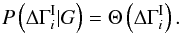 (A.4)However, this is unsatisfactory, as it asserts that the mean intrinsic break is infinite,
  , which is clearly not realistic. As seen below, this results in an unphysical posterior distribution. To remedy this failing, we instead assume that the prior distribution of the intrinsic break is given by a Gaussian, truncated at negative values:
 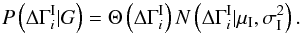 (A.5)In this case the prior is parametrized by two values, μI and σI, which must be either estimated in the problem (i.e., added to the global parameter set G) or specified externally. We will simply assume μI = 0 and derive the results for various reasonable values of σI.
Equation (A.3) can be used to calculate the posterior distribution in the three cases for  discussed above. In the second case, with the prior given by Eq. (A.5), the final integration can be done to give, after applying the formula for the product of Gaussians,
 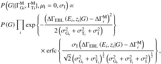 (A.6)where
  is the complementary error function.
It is instructive to examine the two limiting cases of σI = 0 and σI → ∞. In the first case, we arrive at 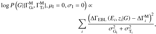 which is exactly the expression that would result from a simple least-squares fit to the measured spectral breaks. In the second case (σI → ∞), we have
 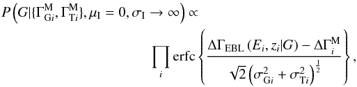 (A.7)which is the same expression as would be derived starting from the prior given by Eq. (A.4). We therefore have an expression that transforms continuously between the two clearly identifiable extremities as a function of σI.
As described in Sect. 3.3, we attempt to derive constraints on two simple models for the EBL: (1) a linear approximation, given by Eq. (1), and (2) a scaling of the EBL model of Franceschini et al. (2008), as described by Eq. (2). In both cases, we assume a uniform prior in the positive region of the parameter space for a, P(a) = Θ(a) and α, P(α) = Θ(α), respectively.
Using either of these, the deficiencies in the model given by Eq. (A.4) is finally evident. Combining Eqs. (2) and (A.7), we get 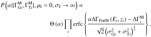 (A.8)The most probable value occurs at α = 0, which is consistent with the assertion in this case that
  .
.
The results in Sect. 3.3 are derived from combining Eqs. (1) (or (2)) and (A.3) with the prior calculated in Appendix B.1 and integrating numerically.
Prediction of mean redshift value ⟨ z ⟩ and upper limit zP < 95% for a give value of ΔΓ.
Appendix A.3: Results with different priors
Table A.1 presents the results obtained with the half-Gaussian prior of Eq. (A.5) (with μI = 0) for four values for the variance of the distribution of the intrinsic break, σI = 0.25,0.5,1.0, and 2.0, and using the prior derived from SSC modeling, illustrated in Fig. B.1.
With increasing value of σI, the most probable value of a or α decreases, since a lower EBL-induced break is needed to reproduce the data. Results derived with values of σI = 0.5 and 1.0 are in good agreement with those from the SSC model.
Appendix A.4: Constraints on the redshift
The Bayesian methodology can also be used to constrain the redshifts of GeV-TeV blazars from their measured spectral breaks. In the case of a single source, Eqs. (A.3) and (2) can be adopted to express the posterior probability for the parameters G = { α,z }, given their priors P(α) and P(z)4. This can then be marginalized over α to give 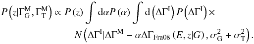 (A.9)The prior for the redshift, P(z), could be estimated from the redshift distribution of detected GeV-TeV detected blazars, i.e., from the values presented in Table 1. However, the true distribution is probably not well represented by the small number of sources detected, so we seek an alternative approach. Another option is to use a flat distribution, which is conservative but also unrealistic. We instead compromise and use the distribution of 2FGL BL Lac objects and unknown AGN. Since Fermi AGN are detected to higher redshifts than those at TeV energies, this should still be a conservative approach. For the prior on the EBL scaling, P(α), we use the positive portion of a Gaussian with mean 1.0 and RMS 0.3, P(α) = Θ(α)N(α | 1.0,0.32). Finally, we use the prior on ΔΓI derived from our SSC simulations, as described above.
The mean redshift and upper limits for some values of ΔΓ, calculated using a typical value of  , are given in Table A.2. The corresponding relation between ⟨ z ⟩ and ΔΓ can be approximated by
  and the relation between zP < 95% and ΔΓ by
Appendix B: Synchrotron self-Compton simulations
Appendix B.1: Determination of the intrinsic break properties
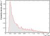 |
Fig. B.1 ΓVHE − ΓHE distribution (red histogram) obtained with the SSC simulations and application of cuts described in the text. |
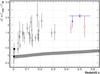 |
Fig. B.2 Value of ΔΓ as a function of the redshift z. The gray line is the break due to redshift effect as computed with the SSC simulation. |
In order to derive a plausible prior probability density for the intrinsic break between HE and VHE for use in the Bayesian model, we produce a set of Monte Carlo simulations of hypothetical BL Lacs using a one-zone SSC model (Band & Grindlay 1985), which is often used to successfully reproduce the time-averaged SEDs from radio to TeV energies.
Parameters used for the SSC simulations.
We assume a spherical emission zone, with a size R, moving at a bulk Doppler factor δ. This region is filled by a uniform magnetic field B, and a population of electrons with a density Ne(γ) is responsible for the synchrotron emission. The synchrotron photons are upscattered by the same population of electrons to produce γ rays.
The distribution of electrons is described by a power law with an exponential cutoff (Lefa et al. 2012), Ne(γ) = N0γp·exp( − γ/γcut). The model therefore has three parameters to describe the electron population (N0, p, and γcut) and four to describe the jet properties (z, R, δ, and B). Among these parameters, R, δ, and N0 have only an achromatic effect, and z produces a small K correction, which is evaluated separately in Appendix B.2. The spectral break is also insensitive to the value of the index p of the electron distribution. The parameters that determine the intrinsic break are therefore B and γcut.
We perform 105 simulations in which the values of B and γcut are uniformly drawn in the range 0.01 < B < 0.5 G and 3 × 10⁴ < γcut < 1 × 10⁷. The other parameters are kept fixed at the values given in Table B.1, which are typical for BL Lacs.
Since only the BL Lac-type SEDs are of interest in this study, simulations have been removed for which the synchrotron emission peaks at energies lower than 10 eV or higher that 10 MeV and which have an HE index of Γ > 2. The distribution of the intrinsic break  , depicted in Figure B.1, has a sharp rise below 0.2 and a long tail at higher break values.
Appendix B.2: Effects of the energy shift due to the distance
The SSC simulations can be used to evaluate the size of the K correction required to account for the redshifting of the intrinsic spectrum into the fixed HE and VHE observation windows. This effect produces a trend of increasing observed ΔΓ with z, even in the absence of EBL absorption.
As before, the SSC parameters are fixed to the values in Table B.1, but with B = 0.1 G and γcut = 1.6 × 10⁵. This produces an intrinsic spectrum with  and
and  , i.e., ΔΓI = 1.19. Simulating the same source with redshifts in the range 10-4 < z < 0.7 and with no EBL absorption leads to an additional component in the observed ΔΓ, which increases with redshift, as depicted in Fig. B.2. This corresponds to the K correction for this intrinsic spectral shape and is too small to explain the trend observed in the data.
The created pairs can also upscatter photons from the cosmic microwave background to high-energy γ-rays (Protheroe 1986) and induce yet another spectral distortion, mostly at energies ~ 100 GeV and below (e.g., Aharonian et al. 2002; D’Avezac et al. 2007), a feature which has currently not been observed (Neronov & Vovk 2010) with instruments sensitive in that energy range.
We define the excess variance of a set of measured quantities xi ± σi to be  .
.
We neglect the dependence of the prior for z on the strength of the EBL (α), i.e., we assume incorrectly that P(z | α) = P(z).
References
- Abdo, A. A., Ackermann, M., Ajello, M., et al. 2009, ApJ, 707, 1310 [NASA ADS] [CrossRef] [Google Scholar]
- Abdo, A. A., Ackermann, M., Ajello, M., et al. 2010a, ApJ, 722, 520 [NASA ADS] [CrossRef] [Google Scholar]
- Abdo, A. A., Ackermann, M., Ajello, M., et al. 2010b, ApJ, 708, 1310 [NASA ADS] [CrossRef] [Google Scholar]
- Abramowski, A., Acero, F., Aharonian, F., et al. 2010, A&A, 516, A56 [NASA ADS] [CrossRef] [EDP Sciences] [Google Scholar]
- Abramowski, A., Acero, F., Aharonian, F., et al. (H.E.S.S. Collaboration) 2012a, A&A, 538, A103 [NASA ADS] [CrossRef] [EDP Sciences] [Google Scholar]
- Abramowski, A., Acero, F., Aharonian, F., et al. 2012b, A&A, 542, A94 [NASA ADS] [CrossRef] [EDP Sciences] [Google Scholar]
- Abramowski, A., Acero, F., Aharonian, F., et al. 2013, A&A, 550, A4 [NASA ADS] [CrossRef] [EDP Sciences] [Google Scholar]
- Acciari, V. A., Aliu, E., Arlen, T., et al. 2010, ApJ, 715, L49 [NASA ADS] [CrossRef] [Google Scholar]
- Acero, F., Aharonian, F., Akhperjanian, A. G., et al. 2010, A&A, 511, A52 [NASA ADS] [CrossRef] [EDP Sciences] [Google Scholar]
- Ackermann, M., Ajello, M., Allafort, A., et al. 2011, ApJ, 743, 171 [NASA ADS] [CrossRef] [Google Scholar]
- Ackermann, M., Ajello, M., Allafort, A., et al. 2012, Science, 338, 1190 [NASA ADS] [CrossRef] [Google Scholar]
- Actis, M., Agnetta, G., Aharonian, F., et al. 2011, Exp. Astron., 32, 193 [NASA ADS] [CrossRef] [Google Scholar]
- Aharonian, F. A., Timokhin, A. N., & Plyasheshnikov, A. V. 2002, A&A, 384, 834 [NASA ADS] [CrossRef] [EDP Sciences] [Google Scholar]
- Aharonian, F., Akhperjanian, A., Beilicke, M., et al. 2003, A&A, 403, 523 [NASA ADS] [CrossRef] [EDP Sciences] [Google Scholar]
- Aharonian, F., Akhperjanian, A. G., Bazer-Bachi, A. R., et al. 2006, Nature, 440, 1018 [NASA ADS] [CrossRef] [PubMed] [Google Scholar]
- Aharonian, F. A., Khangulyan, D., & Costamante, L. 2008, MNRAS, 387, 1206 [NASA ADS] [CrossRef] [Google Scholar]
- Ahrendt, P. 2005, The Multivariate Gaussian Probability Distribution, Tech. Rep. IMM3312, DTU [Google Scholar]
- Aleksić, J., Antonelli, L. A., Antoranz, P., et al. 2011, ApJ, 730, L8 [NASA ADS] [CrossRef] [Google Scholar]
- Aleksić, J., Alvarez, E. A., Antonelli, L. A., et al. 2012a, A&A, 539, A118 [NASA ADS] [CrossRef] [EDP Sciences] [Google Scholar]
- Aleksić, J., Alvarez, E. A., Antonelli, L. A., et al. 2012b, ApJ, 748, 46 [Google Scholar]
- Aliu, E., Aune, T., Beilicke, M., et al. 2011, ApJ, 742, 127 [NASA ADS] [CrossRef] [Google Scholar]
- Aliu, E., Archambault, S., Arlen, T., et al. (VERITAS Collaboration) 2012, ApJ, 750, 94 [NASA ADS] [CrossRef] [Google Scholar]
- Anderhub, H., Antonelli, L. A., Antoranz, P., et al. 2009, ApJ, 704, L129 [NASA ADS] [CrossRef] [Google Scholar]
- Atwood, W. B., Abdo, A. A., Ackermann, M., et al. 2009, ApJ, 697, 1071 [NASA ADS] [CrossRef] [Google Scholar]
- Band, D. L., & Grindlay, J. E. 1985, ApJ, 298, 128 [NASA ADS] [CrossRef] [Google Scholar]
- Benbow, W., & The VERITAS Collaboration. 2011, in Proc 32nd Intl. Cosmic Ray Conf., Beijing [arXiv:1110.0038] [Google Scholar]
- Coppi, P. S., & Aharonian, F. A. 1999, Astropart. Phys., 11, 35 [Google Scholar]
- D’Avezac, P., Dubus, G., & Giebels, B. 2007, A&A, 469, 857 [NASA ADS] [CrossRef] [EDP Sciences] [Google Scholar]
- De Angelis, A., Mansutti, O., Persic, M., & Roncadelli, M. 2009, MNRAS, 394, L21 [NASA ADS] [CrossRef] [Google Scholar]
- Dwek, E., & Krennrich, F. 2005, ApJ, 618, 657 [NASA ADS] [CrossRef] [Google Scholar]
- Essey, W., & Kusenko, A. 2012, ApJ, 751, L11 [NASA ADS] [CrossRef] [Google Scholar]
- Franceschini, A., Rodighiero, G., & Vaccari, M. 2008, A&A, 487, 837 [NASA ADS] [CrossRef] [EDP Sciences] [Google Scholar]
- Gelman, A., Carlin, J. B., Stern, H. S., & Rubin, D. B. 2003, Bayesian Data Analysis, 2nd edn. (Chapman and Hall/CRC) [Google Scholar]
- Hauser, M. G., & Dwek, E. 2001, ARA&A, 39, 249 [NASA ADS] [CrossRef] [Google Scholar]
- Lefa, E., Kelner, S. R., & Aharonian, F. A. 2012, ApJ, 753, 176 [NASA ADS] [CrossRef] [Google Scholar]
- Madau, P., & Pozzetti, L. 2000, MNRAS, 312, L9 [NASA ADS] [CrossRef] [Google Scholar]
- Massaro, E., Tramacere, A., Perri, M., Giommi, P., & Tosti, G. 2006, A&A, 448, 861 [NASA ADS] [CrossRef] [EDP Sciences] [Google Scholar]
- Meyer, M., Raue, M., Mazin, D., & Horns, D. 2012, in High Energy Gamma-Ray Astronomy: 5th International Meeting on High Energy Gamma-Ray Astronomy, AIP Conf. Proc., 1505, 602 [NASA ADS] [CrossRef] [Google Scholar]
- Mori, M. 2009, J. Phys. Soc. Jpn, 78, 78 [NASA ADS] [CrossRef] [Google Scholar]
- Neronov, A., & Vovk, I. 2010, Science, 328, 73 [NASA ADS] [CrossRef] [PubMed] [Google Scholar]
- Orr, M. R., Krennrich, F., & Dwek, E. 2011, ApJ, 733, 77 [NASA ADS] [CrossRef] [Google Scholar]
- Perlman, E. S., Madejski, G., Georganopoulos, M., et al. 2005, ApJ, 625, 727 [NASA ADS] [CrossRef] [Google Scholar]
- Prandini, E., Bonnoli, G., Maraschi, L., Mariotti, M., & Tavecchio, F. 2010, MNRAS, 405, L76 [NASA ADS] [CrossRef] [Google Scholar]
- Prandini, E., Bonnoli, G., & Tavecchio, F. 2012, A&A, 543, A111 [NASA ADS] [CrossRef] [EDP Sciences] [Google Scholar]
- Protheroe, R. J. 1986, MNRAS, 221, 769 [NASA ADS] [Google Scholar]
- Punch, M., Akerlof, C. W., Cawley, M. F., et al. 1992, Nature, 358, 477 [NASA ADS] [CrossRef] [Google Scholar]
- Sitarek, J., & Bednarek, W. 2008, MNRAS, 391, 624 [NASA ADS] [CrossRef] [Google Scholar]
- Stecker, F. W., & Scully, S. T. 2006, ApJ, 652, L9 [NASA ADS] [CrossRef] [Google Scholar]
- Stecker, F. W., & Scully, S. T. 2010, ApJ, 709, L124 [NASA ADS] [CrossRef] [Google Scholar]
- Wakely, S. P., & Horan, D. 2008, in International Cosmic Ray Conference, 3, 1341 [Google Scholar]
- Yang, J., & Wang, J. 2010, A&A, 522, A12 [NASA ADS] [CrossRef] [EDP Sciences] [Google Scholar]
All Tables
Summary of results with the linear parametrization and scaled Franceschini et al. (2008) EBL model obtained with the Bayesian approach described in the text.
Prediction of mean redshift value ⟨ z ⟩ and upper limit zP < 95% for a give value of ΔΓ.
All Figures
|
Fig. 1 Value of ΔΓ as a function of the redshift z. The black line is the theoretical break obtained with the Franceschini et al. (2008) model. The uncertainties due to the energy resolution of IACTs (dark gray), the different threshold energies (medium gray), and the systematic errors of 0.2 (light gray) are shown. The FSRQs and the BL Lacs with uncertain redshift are shown for illustration. |
| In the text | |
|
Fig. 2 Value of ΔΓ as a function of the redshift z. Overlaid are the predicted breaks obtained from the Bayesian fit (simple line), as well as the 95% CL lower limits (hashed area). Left is the linear approximation (Eq. (1)) and right is the scaled model of Fra08 (Eq. (2)). For both models, none of the sources are significantly lower than the 95% CL lower limit. The symbols are descibed in Fig. 1. |
| In the text | |
|
Fig. B.1 ΓVHE − ΓHE distribution (red histogram) obtained with the SSC simulations and application of cuts described in the text. |
| In the text | |
|
Fig. B.2 Value of ΔΓ as a function of the redshift z. The gray line is the break due to redshift effect as computed with the SSC simulation. |
| In the text | |
Current usage metrics show cumulative count of Article Views (full-text article views including HTML views, PDF and ePub downloads, according to the available data) and Abstracts Views on Vision4Press platform.
Data correspond to usage on the plateform after 2015. The current usage metrics is available 48-96 hours after online publication and is updated daily on week days.
Initial download of the metrics may take a while.