© ESO, 2013

1. Introduction

Isotropy of the distributions of matter and light in the Universe is one of the basic assumptions of modern cosmology. The smallness of the temperature anisotropies in the cosmic microwave sky shows that this assumption is an excellent approximation. However, the cosmic microwave sky probes the symmetry of the Universe at the time of photon decoupling and it is interesting to test the assumed isotropy at smaller redshifts. A recent study of various probes at much smaller redshift reveals fluctuations at the per cent level and larger (Gibelyou & Huterer 2012). These can partly be explained by local large scale structure, partly by systematics of the observations, but some of them might be at odds with our understanding of cosmology and call for further investigation.

Complementing the assumption of isotropy with the additional assumption of homogeneity predicts the space-time metric to become of the Robertson-Walker type, predicts the redshift of light z, and predicts the Hubble expansion of the Universe. Then the cosmic luminosity distance-redshift relation for comoving observers and sources becomes $\begin{array}{ccc}{\mathit{d}}_{\mathrm{L}}\mathrm{\left(}\mathit{z}\mathrm{\right)}\mathrm{=}\frac{\mathit{cz}}{{\mathit{H}}_{\mathrm{0}}}\left[\mathrm{1}\mathrm{+}\left(\mathrm{1}\mathrm{-}{\mathit{q}}_{\mathrm{0}}\right)\frac{\mathit{z}}{\mathrm{2}}\right]\mathrm{+}\mathrm{𝒪}\mathrm{(}{\mathit{z}}^{\mathrm{3}}\mathrm{)}\hspace{0.17em}\mathit{,}& & \end{array}$(1)with H₀ and q₀ denoting the Hubble and deceleration parameters, respectively. Note that this prediction holds for arbitrary spatial curvature, any theory of gravity (as long as space-time is described by a single metric) and arbitrary matter content of the Universe.

Assuming the cosmological principle, Seikel & Schwarz (2009) showed that the acceleration of the cosmic expansion can be established in a model independent test (any curvature, any matter content, any dynamics of gravity) at 4.2 sigma from the Union data set of supernovae. One of the assumptions of this test is that supernovae are a fair sample of isotropically distributed standard candles. In Seikel & Schwarz (2009) it was demonstrated that local SNe (z < 0.2) are crucial to this conclusion. These local SNe come from a tiny fraction of the Hubble volume only, thus it is not obvious, if they form a fair sample and if they are sampled from an isotropic and homogeneous distribution. Testing this assumption is the purpose of this work.

A simple test for isotropy relies on comparing Hubble diagrams for pairs of hemispheres. Statistically significant deviations from an isotropic Hubble diagram have been discovered by Schwarz & Weinhorst (2007) at redshifts z < 0.2 in three different data sets. However, the direction of maximal hemispheric asymmetry is close to the equatorial poles, and thus a systematic error in the SN search, observation, analysis or data reduction seems to be plausible.

A more natural direction of anisotropy was identified by Colin et al. (2011). They found out that the low redshift regime (z < 0.06) of the data in the Union 2 catalogue (Amanullah et al. 2010) is barely consistent with ΛCDM at 2 − 3σ because of a bulk flow towards the Shapley supercluster.

Antoniou & Perivolaropoulos (2010) also applied the hemisphere comparison method to the SN Ia data of Union 2 and found a maximum anisotropy, which itself is statistically not significant, but coincides with the bulk velocity flow axis (Feldman et al. 2010; Kashlinsky et al. 2009; Lavaux et al. 2010), cosmic microwave background (CMB) low multipole moments (Bennett et al. 2011; Copi et al. 2010) and the quasar optical polarisation alignment axis (Hutsemekers et al. 2008). Similar directions can be obtained by considering a dynamical dark energy fluid with an anisotropic equation of state in the wCDM model or in Chevallier-Polarski-Linder parametrisation (Cai & Tuo 2012). SNe Ia have also been used by Koivisto & Mota (2008a,b) to test other models of anisotropic dark energy and by Koivisto et al. (2011) to constrain anisotropic curvature. Recently, Mariano & Perivolaropoulos (2012) detected an alignment of supernova dipole asymmetries and a dipole of a locally varying fine structure constant, which can be observed in the Keck+VLT quasar absorber sample. Jackson (2012) found a hemispherical anisotropy in the matter density Ω_m at higher redshifts (0.5 < z ≤ 3.787), where the smallest value of Ω_m points close towards the CMB dipole. An additional tool to test the assumption of isotropy consists of measuring polarisations of different astrophysical sources, as anisotropic expansion has effects in electrodynamics leading to observational consequences (Ciarcelluti 2012).

In the present paper, we analyse directions of maximally asymmetric Hubble expansion constraining its maximum value. Besides, we infer from SN data typical fluctuations of the expansion rate and compare them with expectations for the ΛCDM model. The use of SN data fitted with 4 different light-curve fitters by Hicken et al. (2009) allows us to study systematic effects.

The paper is structured as follows: we explain the method of our test and state the corresponding theoretical expectation on the fluctuations in Sect. 2. We continue with describing the data set, which we will analyse in Sect. 3. Statistical analyses can be found in Sect. 4 and possible systematics will be discussed in Sect. 5. Upper and lower limits on the expansion asymmetry are given in Sect. 6. We conclude in Sect. 7.

2. Hemispherical asymmetries

Our aim is to test whether the Hubble diagram is isotropic. In order to do so, we apply a simple test, that first has been used by Eriksen et al. (2004) to study asymmetries in the CMB anisotropy field, and that Schwarz & Weinhorst (2007) adopted to find anisotropies in SN data. We test the anisotropic cosmic expansion by splitting the sky into hemispheres. Having calculated the Hubble diagrams on both hemispheres separately, one can change the directions of the poles and recalculate the Hubble diagrams on the new hemispheres.

We fit the Hubble diagrams by applying the method of least squares to the distribution of distance moduli of the supernovae, using as a model the relation of the distance modulus to the redshift given by (1) and the definition 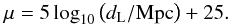$\begin{array}{ccc}\mathit{\mu }\mathrm{=}\mathrm{5}{\log }_{\mathrm{10}}\left({\mathit{d}}_{\mathrm{L}}\mathit{/}\mathrm{Mpc}\right)\mathrm{+}\mathrm{25.}& & \end{array}$(2)Schwarz & Weinhorst (2007) estimated, that the error from truncating Hubble’s law as in (1) is below 10% if one fits only at redshifts z < 0.2. Despite this restriction, this test has the major advantage, that it is model-independent, because (1) follows directly from the cosmological principle and does not contain any terms depending on the curvature, theory of gravity or content of the Universe.

Admittedly, as to go from SN magnitudes m = μ + ℳ to the luminosity distance d_L, one has to know the nuisance parameter $\mathrm{ℳ}\mathrm{\equiv }\mathit{M}\mathrm{-}\mathrm{5}{\log }_{\mathrm{10}}{}^{\mathrm{(}}\mathit{H}_{\mathrm{0}}{}^{\mathrm{)}}\mathrm{+}\mathrm{25}$, which also depends on the absolute magnitude M and hence on the physics of SNe (Perlmutter et al. 1999). We assume that Type Ia SNe are standardisable, thus we treat ℳ as a universal number and use the distance moduli which Hicken et al. (2009) calculated by using four different light-curve fitters with calibrations H₀ = 65 km s^-1 Mpc^-1 and M_B =  −19.46 for SALT, M_B =  −19.44 for SALT II and M_V =  −19.504 for MLCS2k2.

When fitting the Hubble diagrams, we allow H₀ to vary from hemisphere to hemisphere, but keep the deceleration parameter at its best-fit ΛCDM model value. The SN Hubble diagrams considered here do not constrain q₀ well enough, to justify the inclusion of this parameter in the fit.

In a perfectly homogeneous and isotropic Universe we would expect any nontrivial result in the hemispherical asymmetry test to be due to noise and systematics. However, the large scale structure of the Universe is expected to give rise to a small deviation from isotropy. We can estimate the expected amount of fluctuations of the Hubble rate between the hemispheres by estimating their cosmic variance (Turner et al. 1992; Shi 1997; Wang et al. 1998; Li & Schwarz 2008; Wiegand & Schwarz 2012). To measure the difference between the two hemispheres we use the quantity $\frac{{\mathit{H}}_{\mathrm{N}}\mathrm{-}{\mathit{H}}_{\mathrm{S}}}{{\mathit{H}}_{\mathrm{N}}\mathrm{+}{\mathit{H}}_{\mathrm{S}}}$. In the formalism of Wiegand & Schwarz (2012) the Hubble rate on each of the hemispheres is given by the volume average over the local expansion rates. In the linear regime, these are related to the density contrast and therefore the average Hubble rate on a hemisphere is 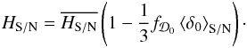$\begin{array}{ccc}{\mathit{H}}_{\mathrm{S}\mathit{/}\mathrm{N}}\mathrm{=}\overline{{\mathit{H}}_{\mathrm{S}\mathit{/}\mathrm{N}}}\left(\mathrm{1}\mathrm{-}\frac{\mathrm{1}}{\mathrm{3}}{\mathit{f}}_{{\mathrm{𝒟}}_{\mathrm{0}}}{⟨{\mathit{\delta }}_{\mathrm{0}}⟩}_{\mathrm{S}\mathit{/}\mathrm{N}}\right)\mathrm{·}& & \end{array}$(3)where the growth rate factor today in the standard ΛCDM model. To first order the anisotropy therefore is $\begin{array}{ccc}\frac{{\mathit{H}}_{\mathrm{N}}\mathrm{-}{\mathit{H}}_{\mathrm{S}}}{{\mathit{H}}_{\mathrm{N}}\mathrm{+}{\mathit{H}}_{\mathrm{S}}}\mathrm{=}\frac{\mathrm{1}}{\mathrm{6}}{\mathit{f}}_{{\mathrm{𝒟}}_{\mathrm{0}}}\left({⟨{\mathit{\delta }}_{\mathrm{0}}⟩}_{\mathrm{S}}\mathrm{-}{⟨{\mathit{\delta }}_{\mathrm{0}}⟩}_{\mathrm{N}}\right)\mathit{.}& & \end{array}$(4)So the ensemble expectation value of the anisotropy is zero at leading order. However, we are interested in the typical fluctuations between different locations in the Universe. Using (4) we find $\begin{array}{ccc}{\mathit{\sigma }}_{\mathrm{A}}\mathrm{=}\mathit{\sigma }\left(\frac{{\mathit{H}}_{\mathrm{N}}\mathrm{-}{\mathit{H}}_{\mathrm{S}}}{{\mathit{H}}_{\mathrm{N}}\mathrm{+}{\mathit{H}}_{\mathrm{S}}}\right)\mathrm{=}\frac{\mathrm{1}}{\mathrm{3}}{\mathit{f}}_{{\mathrm{𝒟}}_{\mathrm{0}}}\sqrt{{\mathit{\sigma }}_{\mathrm{HS}}^{\mathrm{2}}\mathrm{-}{\mathit{\sigma }}_{\mathrm{FS}}^{\mathrm{2}}}& & \end{array}$(5)where $\begin{array}{ccc}{\mathit{\sigma }}_{\mathrm{HS}}^{\mathrm{2}}\mathrm{:}\mathrm{=}{\mathit{\sigma }}^{\mathrm{2}}\left({⟨{\mathit{\delta }}_{\mathrm{0}}⟩}_{\mathrm{N}}\right)\mathrm{=}{\mathit{\sigma }}^{\mathrm{2}}\left({⟨{\mathit{\delta }}_{\mathrm{0}}⟩}_{\mathrm{S}}\right)& & \end{array}$(6)is the matter variance on a hemisphere and 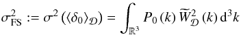$\begin{array}{ccc}{\mathit{\sigma }}_{\mathrm{FS}}^{\mathrm{2}}\mathrm{:}\mathrm{=}{\mathit{\sigma }}^{\mathrm{2}}\left({⟨{\mathit{\delta }}_{\mathrm{0}}⟩}_{\mathrm{𝒟}}\right)\mathrm{=}{\mathrm{\int }}_{R^{\mathrm{3}}}{\mathit{P}}_{\mathrm{0}}\mathrm{(}{\mathit{k}}^{\mathrm{)}}\begin{array}{c}\mathrm{􏽥}\\ {\mathit{W}}_{\mathrm{𝒟}}^{\mathrm{2}}\end{array}\mathrm{(}{\mathit{k}}^{\mathrm{)}}{\mathrm{d}}^{\mathrm{3}}\mathit{k}& & \end{array}$(7)is the matter variance on the full sphere. ${\mathit{P}}_{\mathrm{0}}{}^{\mathrm{\right(}}\mathit{k}^{\mathrm{\left)}}$ is the linear matter power spectrum and $\begin{array}{c}{}_{\mathrm{􏽥}}\\ {\mathit{W}}_{\mathrm{𝒟}}\end{array}{}^{\mathrm{\right(}}\mathit{k}^{\mathrm{\left)}}$ is the Fourier transform of the radial window function ${\mathit{W}}_{\mathrm{𝒟}}{}^{\mathrm{\right(}}\mathit{r}^{\mathrm{\left)}}$ of the domain . This window function is often taken to be of top-hat – or Gaussian – form. To arrive at more precise predictions, however, we shall use in Sect. 3 a shape that describes the actual SN distribution more accurately.

The explicit form of ${\mathit{\sigma }}_{\mathrm{HS}}^{\mathrm{2}}$ is more complicated than the one for the full sphere, because a window function with the geometry of a hemisphere is no longer spherically symmetric. Therefore, the window function has also an angular part in addition to the radial part ${\mathit{W}}_{\mathrm{𝒟}}{}^{\mathrm{\right(}}\mathit{r}^{\mathrm{\left)}}$. We calculate this angular part using a decomposition into spherical harmonics (see Appendix A of Wiegand 2012, for the explicit form). Apart from this angular window function, which is fixed by the requirement that we consider a hemisphere, ${\mathit{\sigma }}_{\mathrm{HS}}^{\mathrm{2}}$ also uniquely depends on ${\mathit{P}}_{\mathrm{0}}{}^{\mathrm{\right(}}\mathit{k}^{\mathrm{\left)}}$ and ${\mathit{W}}_{\mathrm{𝒟}}{}^{\mathrm{\right(}}\mathit{r}^{\mathrm{\left)}}$. Thus, using the fitting formula of Eisenstein & Hu (1998) for the matter power spectrum allows us to estimate the possible anisotropies in a ΛCDM universe in Sect. 3.

3. Supernova data and results

For our analysis, we use the Constitution set (Hicken et al. 2009) supplemented by the positions of the SNe procured from the list of SNe¹ provided by the IAU Central Bureau for Astronomical Telegrams (CBAT). The Constitution set contains a large number of nearby SNe from all the sky (except for the zone of avoidance), whose distance moduli have been obtained by four different light-curve fitters: Multicolor Light Curve Shapes 2k2 (MLCS2k2) (1.7), MLCS2k2(3.1), Spectral Adaptive Light curve Template (SALT) and SALT II. Thus, the Constitution set consists of four samples.

The SALT (Guy et al. 2005) fitter describes light-curves by the peak apparent B-band magnitude ${\mathit{m}}_{\mathit{B}}^{\max }$, the stretch factor s and the colour parameter c. SALT does not distinguish between the intrinsic colour of a SN and the reddening which is caused by dust extinction. Both effects are summarised in c, thus assuming the same colour–magnitude relation for the combination of colour variation and host reddening at low and at high redshift. SALT II (Guy et al. 2007) is similar to SALT, but uses a different spectral template. s has been replaced by a new stretch parameter x₁.

In contrast to the SALT fitters, MLCS2k2 (Jha et al. 2007) includes the intrinsic colour in the shape parameter Δ assuming a broader-bluer and narrower-redder relation. The host-galaxy extinction parameter A_v is then determined separately. This requires assumptions about the dust properties specified by the reddening parameter R_V. In the Milky Way, this parameter has been measured to be R_V = 3.1. We will refer to the MLCS2k2 fitter using this value as MLCS2k2(3.1). Hicken et al. (2009) have determined the reddening parameter, which minimises the scatter in the Hubble diagram, to be R_V = 1.7. In the following, the fitter with this value will be denoted as MLCS2k2(1.7).

While there is a significant overlap of the SNe contained in the samples, not all observed SNe can be found in a specific sample. SNe are rejected due to certain criteria, e.g. if the light-curve fit is not satisfactory or if the light extinction is too high. The different parameters and rejection criteria of the fitters thus lead to a differing number of SNe in the samples. Figure 1 shows the distribution of SNe on the sky for all four samples. In Table 1 the number of SNe with z < 0.2, their mean and median redshifts and their mean σ_μ are listed for all four samples. The SALT sample contains a significantly smaller number of SNe than the other three samples as the stricter rejection criteria from Kowalski et al. (2008) have been adopted.

Fig. 1 Celestial distribution of SNe from Hicken et al. (2009) having redshifts z < 0.2 in galactic coordinates. Black dots represent SNe, that are in all four samples, while green ones cannot be found in the SALT sample, blue ones are only in the MLCS2k2 samples. The MLCS2k2 (RV = 3.1) sample is the only subset, which contains red SNe. We plot in Mollweide projection.

Fig. 2 Colour scaling of all maps drawn for this article. HN − HS denotes the difference in the expansion rates for a pair of hemispheres, $\frac{{\mathit{N}}_{\mathrm{N}}\mathrm{-}{\mathit{N}}_{\mathrm{S}}}{{\mathit{N}}_{\mathrm{N}}\mathrm{+}{\mathit{N}}_{\mathrm{S}}}$ is the corresponding number asymmetry of SNe, $\frac{{\mathit{T}}_{\mathrm{N}}\mathrm{-}{\mathit{T}}_{\mathrm{S}}}{{\mathit{T}}_{\mathrm{N}}\mathrm{+}{\mathit{T}}_{\mathrm{S}}}$ is the asymmetry in dust antenna temperature, $\frac{{\mathrm{\Delta }}_{\mathrm{N}}\mathrm{-}{\mathrm{\Delta }}_{\mathrm{S}}}{{\mathrm{\Delta }}_{\mathrm{N}}\mathrm{+}{\mathrm{\Delta }}_{\mathrm{S}}}$ stands for the asymmetry in the shape parameter of the MLCS2k2 fitter, and $\frac{{\mathit{c}}_{\mathrm{N}}\mathrm{-}{\mathit{c}}_{\mathrm{S}}}{{\mathit{c}}_{\mathrm{N}}\mathrm{+}{\mathit{c}}_{\mathrm{S}}}$ is the colour parameter asymmetry (SALT/SALT II).

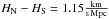
Fig. 3 Hemispherical asymmetry HN − HS in the Hubble rate H0 for each SN Ia fitter. The upper left plot is for MLCS2k2 (1.7), the upper right one is for MLCS2k2 (3.1), below are SALT (left) and SALT II (right). The deceleration parameter is fixed at the value q0 =  −0.601, which one obtains from WMAP (Larson et al. 2011). When the north pole lies in a region with a bluish colour, HN − HS is negative, the red spots denote the directions of positive large asymmetry HN − HS. The Hubble parameter has no anisotropy pointing towards white areas. All plots showing the asymmetry in the Hubble rate have the same scaling. The scale is given in Fig. 2. At the reddest and bluest spots, |HN − HS| = 3.4. We plot directions in galactic coordinates and Mollweide projection. The black line is the equator of the equatorial coordinate system.

In our data analysis, we set the deceleration parameter ${\mathit{q}}_{\mathrm{0}}\mathrm{=}\mathrm{-}{\mathrm{\Omega }}_{\mathrm{\Lambda }}\mathrm{+}\frac{\mathrm{1}}{\mathrm{2}}{\mathrm{\Omega }}_{\mathrm{M}}\mathrm{=}\mathrm{-}\mathrm{0.601}$ according to the seven-year Wilkinson Microwave Anisotropy Probe (WMAP) observations fitted to ΛCDM (Larson et al. 2011).

The effect of our choice of q₀ is not too large: Repeating our test described below for SALT II and fixing q₀ at different values between –1.5 and 0.4, yields values of ${{}^{\mathrm{(}}\mathit{H}_{\mathrm{N}}\mathrm{-}{\mathit{H}}_{\mathrm{S}}{\mathrm{)}}^{}}_{\max }$ which vary almost linearly between 3.20 km s^-1 Mpc^-1 for q₀ =  −1.5 and ${{}^{\mathrm{(}}\mathit{H}_{\mathrm{N}}\mathrm{-}{\mathit{H}}_{\mathrm{S}}{}^{\mathrm{)}}}_{\max }\mathrm{=}\mathrm{2.55}$ km s^-1 Mpc^-1 for q₀ = 0.4.

As said in Sect. 1, we carry out a χ²-fit to adjust the Hubble parameters H_N(ℓ,b) on the hemisphere identified by its pole (ℓ,b) and H_S(ℓ,b) on the complementary hemisphere such that the distance moduli modelled by (2) and related to redshift data by (1) fits the distance moduli given in Hicken et al. (2009) best. We divide the sky into a 1° × 1° grid. Each grid point can be regarded as the pole (ℓ,b) of a hemisphere. We determine the Hubble parameter H_N(ℓ,b) and subtract from it the Hubble parameter H_S(ℓ,b) of the opposite side. The resulting deviations in H₀ are plotted for each light-curve fitter in Fig. 3.

The asymmetry maps for the SALT fitter exhibits several small local extrema in H_N − H_S, which look like noise, while the maps obtained with the MLCS2k2 fitters and SALT II are similar to each other: the white areas, which denote small deviations in the Hubble parameter, have similar shapes, and the directions of maximum asymmetry are also similar, as can be verified in Table 2. Table 2 also shows, that the maxima of $\frac{{\mathit{H}}_{\mathrm{N}}\mathrm{-}{\mathit{H}}_{\mathrm{S}}}{{\mathit{H}}_{\mathrm{N}}\mathrm{+}{\mathit{H}}_{\mathrm{S}}}$ for the MLCS2k2 fitters and SALT II are well above 2% and hence larger than the fluctuations σ_A due to cosmic variance (cf. end of this section). MLCS2k2(1.7) and SALT II yield almost the same directions of maximum asymmetry. The maximally asymmetric direction in the MLCS2k2(3.1) is located in the same quadrant as the previous ones, whilst the direction found in the SALT data is far from the others. One finds also a much smaller value of $\frac{{\mathit{H}}_{\mathrm{N}}\mathrm{-}{\mathit{H}}_{\mathrm{S}}}{{\mathit{H}}_{\mathrm{N}}\mathrm{+}{\mathit{H}}_{\mathrm{S}}}\mathrm{=}\mathrm{1.54}\mathrm{\%}$ using the SALT data.

For a correct interpretation of these anisotropies, we need to compare them to what we expect by cosmic variance. In a statistically homogeneous and isotropic ΛCDM model, the average hemispherical asymmetry is zero. A particular realisation, however, will have an asymmetry. The broadness of the distribution of these asymmetries around zero, is the cosmic variance for the hemispherical asymmetry. We use (5) to estimate it for the four samples. To arrive at reliable predictions for the expected fluctuations in the anisotropy, we have to account for the incompleteness of the sampling of the hemispheres by the supernovae. To this end, we use a radial window function that is adapted to the shape of the redshift distribution of the SNe. We show this redshift distribution in Fig. 4 together with the results of a fit with the ansatz Ar²/⁽1 + Br⁴⁾. We use this shape as the radial window function ${\mathit{W}}_{\mathrm{𝒟}}{}^{\mathrm{\right(}}\mathit{r}^{\mathrm{\left)}}\mathrm{\propto }\mathit{A}\mathit{/}{}^{\mathrm{(}}\mathrm{1}\mathrm{+}\mathit{B}{\mathit{r}}^{\mathrm{4}}{}^{\mathrm{)}}$ in the evaluation of (6) and (7).

Plugging the resulting values for ${\mathit{\sigma }}_{\mathrm{HS}}^{\mathrm{2}}$ and ${\mathit{\sigma }}_{\mathrm{FS}}^{\mathrm{2}}$ into (5), we therefore arrive at a value of about 0.7% as shown in Table 4. Note that this is the expectation value for a randomly fixed direction, not for the direction of maximum asymmetry. We checked if the shape of the radial window function is important by using different forms, including a simple interpolation of the distribution of SN. The values varied between 0.6% and 1.0% indicating that, in any case, the cosmic variance is well below 2%.

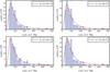Fig. 4 Radial distribution of the supernovae in the MLCS2k2 (1.7) (top left), MLCS2k2 (3.1) (top right), SALT (bottom left) and SALT II (bottom right) data set. The red dashed lines illustrate the radial window functions which we use in our calculations for the expected fluctuations.

On the other hand, Table 1 tells us, that the mean measurement uncertainty σ_μ of the distance modulus is approximately 0.2 mag and that the number of SNe with z < 0.2 is around 200 for the MLCS2k2 data. Thus, we calculate the Hubble parameters with roughly 100 objects per hemisphere, reducing the overall uncertainty in μ to an approximate value of 0.02, which relates to an uncertainty in the Hubble parameter of the order of 0.01.

Hence, the sensitivity of this test applied to the Constitution set is at the same order as the expected fluctuations of ΛCDM, which we therefore cannot see. However, more extreme models would stick out.

4. Statistical analysis

Having found asymmetries, we want to focus on the question of the likeliness of the maximal asymmetry observed on the sky. Therefore, we performed the following analyses.

4.1. Scrambled data

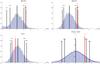Fig. 5 Histograms of the maximal hemispherical asymmetry in the Hubble rate H0 after scrambling 16 000 times the positions of SNe in the MLCS2k2 (1.7) (top left), MLCS2k2 (3.1) (top right), SALT (bottom left) and SALT II (bottom right) data sets. Corresponding to Fig. 3, the deceleration parameter q0 =  −0.601 is fixed. The red line denotes the value one gets by analysing the original data from Hicken et al. (2009), the dashed lines denote the quantiles.

In our first approach we do not relate a SN from the Constitution set to its original position from the CBAT list, but relocate it at the position of another random SN, that is also part of the same sample of SNe. We repeat the procedures described in the previous section for 16 000 realisations, which were generated by scrambling the positions. Thereafter, we again maximise the asymmetries in H_N − H_S, but as to save computing time, we do not calculate the asymmetry in every grid point but first evaluate the hemispherical Hubble asymmetry at 10 different random positions and then use the maximum of these as a start position (ℓ,b)₀ for the simulated annealing method described in Häggström (2002). In this method a Metropolis chain is simulated by determining the Hubble asymmetry on a randomly picked neighbouring point (ℓ,b)_n + 1 = (ℓ_n ± 1°,b_n) or (ℓ,b)_n + 1 = (ℓ_n,b_n ± 1°). The new position (ℓ,b)_n + 1 is either accepted with a probability $\begin{array}{ccc}{\mathit{p}}_{\mathrm{acc}}\mathrm{=}\begin{array}{c}\min \end{array}\begin{array}{c}\mathrm{⎧}\\ \mathrm{⎪}\\ \mathrm{⎪}\\ \mathrm{⎪}\\ \mathrm{⎨}\\ \mathrm{⎪}\\ \mathrm{⎪}\\ \mathrm{⎪}\\ \mathrm{⎩}\end{array}\frac{\exp \mathrm{(}\frac{\mathrm{1}}{{\mathit{T}}_{\mathit{n}\mathrm{+}\mathrm{1}}}\frac{{\mathit{H}}_{\mathrm{N}}\mathrm{-}{\mathit{H}}_{\mathrm{S}}}{{\mathit{H}}_{\mathrm{N}}\mathrm{+}{\mathit{H}}_{\mathrm{S}}}\mathrm{(}\mathit{\ell ,b}{\mathrm{)}}_{\mathit{n}\mathrm{+}\mathrm{1}}\mathrm{)}}{\exp \mathrm{(}\frac{\mathrm{1}}{{\mathit{T}}_{\mathit{n}\mathrm{+}\mathrm{1}}}\frac{{\mathit{H}}_{\mathrm{N}}\mathrm{-}{\mathit{H}}_{\mathrm{S}}}{{\mathit{H}}_{\mathrm{N}}\mathrm{+}{\mathit{H}}_{\mathrm{S}}}\mathrm{(}\mathit{\ell ,b}{\mathrm{)}}_{\mathit{n}}\mathrm{)}}\mathit{,}\mathrm{1}\begin{array}{c}\mathrm{⎫}\\ \mathrm{⎪}\\ \mathrm{⎪}\\ \mathrm{⎪}\\ \mathrm{⎬}\\ \mathrm{⎪}\\ \mathrm{⎪}\\ \mathrm{⎪}\\ \mathrm{⎭}\end{array}& & \end{array}$(8)or rejected with 1 − p_acc, i.e. (ℓ,b)_n + 1 = (ℓ,b)_n. The algorithm converges to the position lim_n → ∞(ℓ,b)_n = (ℓ,b)_max at which the hemispherical Hubble asymmetry is maximised, as long as ${\mathit{T}}_{\mathit{n}}\mathrm{\propto }\frac{\mathrm{1}}{\ln \mathrm{\left(}\mathit{n}\mathrm{\right)}}$ (Geman & Geman 1984). The algorithm is trained to find the same Hubble asymmetry values as in Table 2 with the same accuracy. Out of 10 runs, we identified the maximum number of steps needed to obtain these values and we chose a slightly higher number of steps, after which we truncate the Metropolis chain and save the highest expansion asymmetry appearing therein.

Assuming a perfectly isotropic Hubble expansion, any deviation from hemispherical symmetry would be due to selection effects. Thus scrambling the original data yields an estimate of the distribution one would expect for an isotropic universe, which is measured with the true selection function. Moreover, no model has to be adopted for this test.

The results are visualised in the histograms of Fig. 5. There, one can see again a distinction between the results for the SALT and all the other data samples: the maximum asymmetry in H₀ for the SALT data set is a fair realisation of this Monte Carlo procedure, whilst between 90 and 95% of the maxima of all Monte Carlo realisations are smaller than the asymmetry in the Hubble diagrams for the other light-curve fitters.

4.2. Distance modulus Monte Carlo

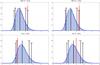Fig. 6 Histograms of the maximum asymmetry in H0 found in 16 000 different realisations of the distance modulus Monte Carlo, applied on the MLCS2k2 1.7, MLCS2k2 3.1, SALT and SALT II data sample, and the respective probability density functions of a generalised extreme value distribution. The distance moduli in the simulated data are normally distributed around their theoretically calculated values with the original measurement errors σμi as standard deviation.

As we filled in the previous analysis observed positions with observed SNe, the simulated data can also be affected by an anisotropic distribution of observed SNe. Another way to check whether the asymmetries are significant is to repeat the following procedure:

• 1.

  We generate a data set, in which we keep the positions andredshifts of each SN, but the distance modulus μ is calculated from its redshift z according to (2), where we assume the WMAP ΛCDM values q₀ =  −0.601 and H₀ = 71.0 km s^-1 Mpc^-1 from Larson et al. (2011).

• 2.

  We simulate “observations” with uncertainties of measurement as a Gaussian distribution , where the expectation value μ equals the previously calculated distance modulus μ and the standard deviation σ equals the measurement uncertainty σ_μi of the distance modulus of the ith SN in the original data set.

• 3.

  We maximise again the anisotropy H_N − H_S in the simulated data set by dint of the simulated annealing method (Häggström 2002).

As the Hubble parameter is normally distributed, and thence the difference H_N − H_S as well, we expect the maximum asymmetry in H₀ to obey a generalised extreme value distribution², due to the Theorem of Fisher & Tippett (1928) and Gnedenko (1943). The probability density function of which with location parameter μ, scale parameter σ and shape parameter ξ ≠ 0 is given by $\begin{array}{ccc}\mathit{f}\mathrm{\left(}\mathit{x}\mathrm{;}\mathit{\mu ,\sigma ,\xi }\mathrm{\right)}\mathrm{=}\frac{\mathrm{1}}{\mathit{\sigma }}{\left[\mathrm{1}\mathrm{+}\mathit{\xi }\left(\frac{\mathit{x}\mathrm{-}\mathit{\mu }}{\mathit{\sigma }}\right)\right]}^{\mathrm{-}\mathrm{1}\mathit{/}\mathit{\xi }\mathrm{-}\mathrm{1}}{\mathrm{e}}^{\mathrm{-}{\left[\mathrm{1}\mathrm{+}\mathit{\xi }\left(\frac{\mathit{x}\mathrm{-}\mathit{\mu }}{\mathit{\sigma }}\right)\right]}^{\mathrm{1}\mathit{/}\mathit{\xi }}}\mathit{.}& & \end{array}$(9)The maximum likelihood parameter estimates can be found in Table 3. For an infinite number of realisations, we would expect ξ = 0, also known as Gumbel distribution. As shown in Table 3, |ξ| ≪ 1.

The resulting histograms (Fig. 6) show statistical significance for the anisotropies found in the MLCS2k2 data, which are higher than 95% of the anisotropies in the simulated data, but they show no significance for the SALT and SALT II asymmetries. The distribution for MLCS2k2 is narrower than the others, because the SALT sample contains less SNe and because SALT II yields larger errors for the distance moduli.

As to study how improving measurements of μ_i affects the usefulness of our hemispheric asymmetry test, we repeat 5000 distance modulus Monte Carlos, but we replace σ_μ by σ_μ/2. We can so show, that if the measurement uncertainty of the distance moduli of every single supernova can be halved, the Hubble asymmetries are expected to be much smaller. Fitting again a generalised extreme value distribution, the maximum likelihood location parameters would amount 1.09 km s^-1 Mpc^-1 and 1.24 km s^-1 Mpc^-1 for MLCS2k2 (3.1) and SALT II respectively. The observed values would lie at the 1 − 10^-6 and 1 − 4 × 10^-5 quantiles for the MLCS2k2 (3.1) and SALT II light-curve fitters. We hope, this will encourage observers to further reduce measurement errors, as it also improves this test considerably.

4.3. Comparison with cosmic variance

Finally, we want to determine the fluctuations of the hemispherical asymmetry around its average, for a random orientation of the hemispheres. To calculate these fluctuations, we pick 10 000 random positions (ℓ, b) in the sky. Each position so determines the north pole of a random sphere. We split this sphere into its northern and southern hemisphere and calculate from the Constitution set the hemispherical Hubble asymmetry $\frac{{\mathit{H}}_{\mathrm{N}}\mathrm{-}{\mathit{H}}_{\mathrm{S}}}{{\mathit{H}}_{\mathrm{N}}\mathrm{+}{\mathit{H}}_{\mathrm{S}}}$ of this randomly oriented sphere. The variance of the Hubble asymmetry for the 10 000 spheres is then the desired fluctuation.

To sample the random north pole positions (ℓ, b), we employ a restriction: if we chose them from the whole sky [ℓ uniformly distributed, $\mathrm{pdf}\mathrm{\left(}\mathit{b}\mathrm{\right)}\mathrm{=}\frac{\mathrm{1}}{\mathrm{2}}\cos \mathrm{\left(}\mathit{b}\mathrm{\right)}$], for each position where we take (ℓ, b) to be the north pole of our random sphere, we would also have a random sphere in the sample where (ℓ, b) is the south pole, because we chose the position (π + ℓ, − b) as a north pole. So in order for the average to be the typical asymmetry for random orientation, we have to restrict the choice of random north pole positions (ℓ, b) to one hemisphere of the sky.

In order not to miss a direction of high anisotropy, we do three runs for orthogonal directions in the sky that we take as the poles of the hemispheres on which we sample our random positions (ℓ, b). In the first run, we generate only positions (ℓ, b) on the northern galactic hemisphere, in the second run positions are restricted to the western hemisphere and in the third repetition the generated (ℓ, b) are located on the hemisphere towards the galactic centre.

Table 4 compares the empirical root mean square fluctuations σ_emp of the hemispherical Hubble asymmetry determined by this prescription with the fluctuations in the Hubble asymmetry due to cosmic variance σ_A. Under the assumption that each configuration of SN in the sphere obtained by the random choice of its north pole position represents a realisation of the stochastic process that generates the SN distribution, σ_emp should give an estimate of σ_A. Table 4 shows, that their values indeed are quite comparable. Only the empirical values obtained with MLCS2k2 (1.7) and SALT II are slightly higher than expected from this reasoning.

5. Systematics

5.1. Equatorial hemispheres

In this section we are concerned with the question how unlikely is the asymmetry observed towards a fixed direction on the sky. Therefore, we carry out again the distance modulus Monte Carlo, but now we do not maximise the anisotropy, but we calculate the differences in the Hubble parameters of the equatorial hemispheres. The results all look like those obtained from SALT II (Fig. 7), where the measured value ${\mathit{H}}_{\mathrm{N}}\mathrm{-}{\mathit{H}}_{\mathrm{S}}\mathrm{=}\mathrm{1.15}\frac{\mathrm{km}}{\mathrm{s}\hspace{0.17em}\mathrm{Mpc}}\mathrm{=̂}\frac{{\mathit{H}}_{\mathrm{N}}\mathrm{-}{\mathit{H}}_{\mathrm{S}}}{{\mathit{H}}_{\mathrm{N}}\mathrm{+}{\mathit{H}}_{\mathrm{S}}}\mathrm{=}\mathrm{0.88}\mathrm{\%}$ lies within the 90% confidence interval of the resulting distribution. The corresponding values for MLCS2k2 1.7 and 3.1, as well as for SALT are $\mathrm{1.00}\frac{\mathrm{km}}{\mathrm{s}\hspace{0.17em}\mathrm{Mpc}}$, $\mathrm{1.25}\frac{\mathrm{km}}{\mathrm{s}\hspace{0.17em}\mathrm{Mpc}}$ and $\mathrm{-}\mathrm{0.45}\frac{\mathrm{km}}{\mathrm{s}\hspace{0.17em}\mathrm{Mpc}}$ or accordingly 0.76%, 0.96% and –0.34%. These values are all smaller than the cosmic variance. Thence and because the values lie within their corresponding 90% confidence intervals, this test does not support that the observation strongly depend on Earth related effects.

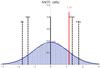Fig. 7 Histogram with the resulting differences between the Hubble rate on the northern equatorial hemisphere HN and the southern equatorial hemisphere HS obtained from 16 000 runs of the distance modulus Monte Carlo. The red line indicates the measured value ${\mathit{H}}_{\mathrm{N}}\mathrm{-}{\mathit{H}}_{\mathrm{S}}\mathrm{=}\mathrm{1.15}\frac{\mathrm{km}}{\mathrm{s}\hspace{0.17em}\mathrm{Mpc}}$ obtained from the SALT II data set. We also plotted a normal distribution with μ = 0.00 and σ = 1.07.

5.2. Number asymmetry

Fig. 8 Hemispherical asymmetry $\frac{{\mathit{N}}_{\mathrm{N}}\mathrm{-}{\mathit{N}}_{\mathrm{S}}}{{\mathit{N}}_{\mathrm{N}}\mathrm{+}{\mathit{N}}_{\mathrm{S}}}$ in the number Ni of SNe on the Hemisphere labelled with i. The plots are adjusted in the same way as Fig. 3. The maximum value, which defines the scale, is 0.52.

As already mentioned, the asymmetries in H₀ can be due to incomplete SNe Ia observations in some directions. Therefore, we plotted the difference between the number of SNe on both hemispheres similarly to Fig. 3. These plots (Fig. 8) show anisotropies in $\frac{{\mathit{N}}_{\mathrm{N}}\mathrm{-}{\mathit{N}}_{\mathrm{S}}}{{\mathit{N}}_{\mathrm{N}}\mathrm{+}{\mathit{N}}_{\mathrm{S}}}$, but they do not agree with any asymmetry map in Fig. 3. The asymmetry in the SN distribution is minimal near the Earth’s equator and maximal approximately at its poles. Also the white region, in which the number asymmetry is zero, follows the equatorial equator. This is not the case in Fig. 3.

Although the maximal asymmetries in the number of SNe is around 50% in all data sets, the number asymmetries for the hemispheres that give the maximal expansion anisotropies (cf. Table 2) are much smaller for MLCS2k2 and SALT II (MLCS2k2 1.7: –4.8%, MLCS2k2 3.1: –20.2%, SALT II: –10.6%). Only SALT manifests a comparably high number asymmetry between the hemispheres of maximum expansion asymmetry, that is to say 46.9%, even though it is the most isotropic subsample in terms of Hubble asymmetry.

For that reason we cannot think of the incompleteness of the SN data being the main explanation of asymmetries found in the Hubble expansion.

5.3. Quality of fit

Another possible systematic effect could be, that the quality of our fits is different in different directions. We have verified, that the asymmetries in $\frac{{\mathit{\chi }}^{\mathrm{2}}}{\mathrm{d}\mathit{.}\mathrm{o}\mathit{.}\mathrm{f}\mathit{.}}$ are also not aligned with the asymmetries in H₀.

5.4. Dust asymmetry

We assume, that the Universe is isotropic on large scales. The foreground, like dust within our galaxy, is not isotropic and therefore a possible explanation of apparent anisotropic expansion.

For the comparison with galactic dust, we brought the Schlegel dust map (Schlegel et al. 1998) into the same form as our other maps. The result can be seen in Fig. 9. This map has no similarities with Fig. 3, thus, we can also exclude dust as a reason for apparent anisotropic cosmic expansion.

5.5. Shape asymmetry

The MLCS2k2 light-curve fitter uses the light-curve shape to remove the influence of dust from the distance measurement (Riess et al. 1998). As Hicken et al. (2009) provides the shape parameter of each SN, we also plot the weighted difference $\frac{{\mathrm{\Delta }}_{\mathrm{N}}\mathrm{-}{\mathrm{\Delta }}_{\mathrm{S}}}{{\mathrm{\Delta }}_{\mathrm{N}}\mathrm{+}{\mathrm{\Delta }}_{\mathrm{S}}}$ between the average shape parameters Δ of each hemisphere (see Fig. 10). These plots also do not reproduce the shapes of the asymmetry map of H₀ (Fig. 3).

5.6. Colour asymmetry

SALT and SALT II use a colour parameter to get rid of dust (Guy et al. 2005, 2007). We tested the asymmetries in the colour parameter in the same way as those in the shape parameter. The resulting maps are shown in Fig. 11. The SALT data set shows directions in which the colour parameter is obviously asymmetric, as against irregular asymmetries of the colour parameter in the SALT II data.

6. Limits on expansion asymmetry

As to find limits on the Hubble expansion asymmetry of the local Universe, we draw realisations from the SN magnitudes and redshifts given the reported measurements with errors. We then compute the asymmetry of the original direction of maximum asymmetry given in Table 2. After 5400 realisations, we enumerate the 95% quantile H₉₅, which can be regarded as an upper limit on the expansion asymmetry, as well as the 5% quantile H₅. In an isotropic universe, all measurements of the Hubble asymmetry should agree with ΔH/H = 0 at every position. Hence, a positive H₅ cannot be explained by statistical fluctuations alone.

H₅ and H₉₅ can be found for every light-curve fitter in Table 5. SALT is consistent with an isotropic local Universe, whilst the other light-curve fitters provide evidence for real anisotropies. MLCS2k2 (3.1) features an H₅, which is even comparably high as our expectations for typical fluctuations due to large scale structure.

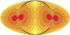Fig. 9 Hemispherical asymmetry in the antenna temperature of the foreground dust extracted from Schlegel et al. (1998). The maximum asymmetry is 0.14 mK.

Fig. 10 Asymmetry $\frac{{\mathrm{\Delta }}_{\mathrm{N}}\mathrm{-}{\mathrm{\Delta }}_{\mathrm{S}}}{{\mathrm{\Delta }}_{\mathrm{N}}\mathrm{+}{\mathrm{\Delta }}_{\mathrm{S}}}$ of the shape parameter Δ. The scaling is defined by the maximum value of 0.57. The plot on the left is for MLCS2k2(1.7), the other one for MLCS2k2(3.7).

Fig. 11 Asymmetry $\frac{{\mathit{c}}_{\mathrm{N}}\mathrm{-}{\mathit{c}}_{\mathrm{S}}}{{\mathit{c}}_{\mathrm{N}}\mathrm{+}{\mathit{c}}_{\mathrm{S}}}$ of the colour parameter. The maximum value amounts to 0.64. The plot on the left hand side shows the colour asymmetry in the SALT data, the right one in SALT II.

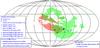Fig. 12 95% confidence level contours of the SALT II (green lines) and MLCS2k2(3.1) (red lines) maximum asymmetry directions (MLCS2k2 (3.1) ■, SALT II •) as well as 90% confidence level contours (filled green and filled red respectively, filled dark green where they coincide) compared with directions of anisotropies in SN data from Antoniou & Perivolaropoulos (2010) (z < 1.4) □, Cai & Tuo (2012) (z < 0.2 ▴, z < 1.4 °), Colin et al. (2011) (z < 0.2 ▾), Mariano & Perivolaropoulos (2012) ▵ and Schwarz & Weinhorst (2007) (data set A ◆, B ♣, D ♠), and with the direction of the CMB dipole moment ♡ (Lineweaver et al. 1996), the Shapley supercluster ▿ (Raychaudhury 1989), the cold spots I ★ (Bennett et al. 2011) and II detected in WMAP data ◇ (Cruz et al. 2007), and the South Equatorial Pole S.

In Fig. 12, we plot the contours of the 5% quantiles of the MLCS2k2 (3.1) and SALT II as error contours of the direction of maximum Hubble asymmetry. Both data sets agree with the expansion being fastest into the direction of the WMAP cold spot I reported by Bennett et al. (2011).

The H₉₅ values provide upper limits on the anisotropy of the Hubble expansion. The least stringent upper limit is found from MLCS2k2 (3.1), namely $\frac{{\mathit{H}}_{\mathrm{N}}\mathrm{-}{\mathit{H}}_{\mathrm{S}}}{{\mathit{H}}_{\mathrm{N}}\mathrm{+}{\mathit{H}}_{\mathrm{S}}}\mathit{<}\mathrm{0.038}$ at 95% C.L.

7. Conclusion

We analyse hemispherical asymmetries ΔH/H = (H_N − H_S)/(H_N + H_S) in the Hubble expansion rate at redshifts z < 0.2 in SN data of the Constitution set published by Hicken et al. (2009). The observed hemispherical asymmetry of the Hubble expansion is in agreement with the order of magnitude that can be expected by cosmic variance in a ΛCDM universe, but is inconsistent with the assumption of perfect isotropy and homogeneity.

However, the Hubble asymmetry in the direction of maximal asymmetry as identified by the MLCS2k2 light curve fitter, is at 95% C.L. larger than in a random realisation of distance modulus observations. All light-curve fitters, bar SALT, establish their respective asymmetric directions at 90% C.L. in terms of data scrambling. Figure 12 shows their agreement with directions reported by Cai & Tuo (2012); Mariano & Perivolaropoulos (2012) and Schwarz & Weinhorst (2007), which are in the vicinity to the WMAP cold spot I (Bennett et al. 2011). Inoue & Silk (2007) explained observed large-angle CMB anomalies with a pair of local dust-filled voids. These would cause both a cold spot in CMB data and fluctuations in the locally measured Hubble constant as large as 2–4%. Our measured Hubble anisotropy of ΔH/H ~ 0.026 agrees with this finding. Despite the fact that it is significant, we so conclude that the anisotropy does not contradict global isotropy, because firstly it can be explained by local structure, secondly we only analysed local SNe and thirdly it matches our predictions of typical fluctuations in a ΛCDM background.

Admittedly, our test is not sensitive enough to see if the 1% asymmetry detected for random hemispheres is due to ΛCDM-fluctuations of the local structure. So it should be repeated, when a full sky survey comprising approximately 2000 SNe becomes available, or when the errors of individual SNe could be reduced by about a factor of 2. But nevertheless we can constrain the expansion asymmetry of the local Universe to be less than 3.8% at 95% C.L. using most conservatively the results obtained with the MLCS2k2 (3.1) light-curve fitter.

Acknowledgments

We thank Marek Kowalski for valuable discussions. We acknowledge the use of the List of Supernovae provided by the IAU Central Bureau for Astronomical Telegrams (http://www.cbat.eps.harvard.edu/lists/Supernovae.html). We acknowledge financial support from Deutsche Forschungsgemeinschaft under grants IRTG 881 and RTG 1620. M.S. is supported by the South African Square Kilometre Array Project.

References

All Tables

All Figures

	Fig. 1 Celestial distribution of SNe from Hicken et al. (2009) having redshifts z < 0.2 in galactic coordinates. Black dots represent SNe, that are in all four samples, while green ones cannot be found in the SALT sample, blue ones are only in the MLCS2k2 samples. The MLCS2k2 (RV = 3.1) sample is the only subset, which contains red SNe. We plot in Mollweide projection.
In the text

Fig. 2 Colour scaling of all maps drawn for this article. HN − HS denotes the difference in the expansion rates for a pair of hemispheres, $\frac{{\mathit{N}}_{\mathrm{N}}\mathrm{-}{\mathit{N}}_{\mathrm{S}}}{{\mathit{N}}_{\mathrm{N}}\mathrm{+}{\mathit{N}}_{\mathrm{S}}}$ is the corresponding number asymmetry of SNe, $\frac{{\mathit{T}}_{\mathrm{N}}\mathrm{-}{\mathit{T}}_{\mathrm{S}}}{{\mathit{T}}_{\mathrm{N}}\mathrm{+}{\mathit{T}}_{\mathrm{S}}}$ is the asymmetry in dust antenna temperature, $\frac{{\mathrm{\Delta }}_{\mathrm{N}}\mathrm{-}{\mathrm{\Delta }}_{\mathrm{S}}}{{\mathrm{\Delta }}_{\mathrm{N}}\mathrm{+}{\mathrm{\Delta }}_{\mathrm{S}}}$ stands for the asymmetry in the shape parameter of the MLCS2k2 fitter, and $\frac{{\mathit{c}}_{\mathrm{N}}\mathrm{-}{\mathit{c}}_{\mathrm{S}}}{{\mathit{c}}_{\mathrm{N}}\mathrm{+}{\mathit{c}}_{\mathrm{S}}}$ is the colour parameter asymmetry (SALT/SALT II).

In the text

Fig. 3 Hemispherical asymmetry HN − HS in the Hubble rate H0 for each SN Ia fitter. The upper left plot is for MLCS2k2 (1.7), the upper right one is for MLCS2k2 (3.1), below are SALT (left) and SALT II (right). The deceleration parameter is fixed at the value q0 =  −0.601, which one obtains from WMAP (Larson et al. 2011). When the north pole lies in a region with a bluish colour, HN − HS is negative, the red spots denote the directions of positive large asymmetry HN − HS. The Hubble parameter has no anisotropy pointing towards white areas. All plots showing the asymmetry in the Hubble rate have the same scaling. The scale is given in Fig. 2. At the reddest and bluest spots, |HN − HS| = 3.4. We plot directions in galactic coordinates and Mollweide projection. The black line is the equator of the equatorial coordinate system.

In the text

	Fig. 4 Radial distribution of the supernovae in the MLCS2k2 (1.7) (top left), MLCS2k2 (3.1) (top right), SALT (bottom left) and SALT II (bottom right) data set. The red dashed lines illustrate the radial window functions which we use in our calculations for the expected fluctuations.
In the text

Fig. 5 Histograms of the maximal hemispherical asymmetry in the Hubble rate H0 after scrambling 16 000 times the positions of SNe in the MLCS2k2 (1.7) (top left), MLCS2k2 (3.1) (top right), SALT (bottom left) and SALT II (bottom right) data sets. Corresponding to Fig. 3, the deceleration parameter q0 =  −0.601 is fixed. The red line denotes the value one gets by analysing the original data from Hicken et al. (2009), the dashed lines denote the quantiles.

In the text

Fig. 6 Histograms of the maximum asymmetry in H0 found in 16 000 different realisations of the distance modulus Monte Carlo, applied on the MLCS2k2 1.7, MLCS2k2 3.1, SALT and SALT II data sample, and the respective probability density functions of a generalised extreme value distribution. The distance moduli in the simulated data are normally distributed around their theoretically calculated values with the original measurement errors σμi as standard deviation.

In the text

Fig. 7 Histogram with the resulting differences between the Hubble rate on the northern equatorial hemisphere HN and the southern equatorial hemisphere HS obtained from 16 000 runs of the distance modulus Monte Carlo. The red line indicates the measured value ${\mathit{H}}_{\mathrm{N}}\mathrm{-}{\mathit{H}}_{\mathrm{S}}\mathrm{=}\mathrm{1.15}\frac{\mathrm{km}}{\mathrm{s}\hspace{0.17em}\mathrm{Mpc}}$ obtained from the SALT II data set. We also plotted a normal distribution with μ = 0.00 and σ = 1.07.

In the text

	Fig. 8 Hemispherical asymmetry $\frac{{\mathit{N}}_{\mathrm{N}}\mathrm{-}{\mathit{N}}_{\mathrm{S}}}{{\mathit{N}}_{\mathrm{N}}\mathrm{+}{\mathit{N}}_{\mathrm{S}}}$ in the number Ni of SNe on the Hemisphere labelled with i. The plots are adjusted in the same way as Fig. 3. The maximum value, which defines the scale, is 0.52.
In the text

	Fig. 9 Hemispherical asymmetry in the antenna temperature of the foreground dust extracted from Schlegel et al. (1998). The maximum asymmetry is 0.14 mK.
In the text

	Fig. 10 Asymmetry $\frac{{\mathrm{\Delta }}_{\mathrm{N}}\mathrm{-}{\mathrm{\Delta }}_{\mathrm{S}}}{{\mathrm{\Delta }}_{\mathrm{N}}\mathrm{+}{\mathrm{\Delta }}_{\mathrm{S}}}$ of the shape parameter Δ. The scaling is defined by the maximum value of 0.57. The plot on the left is for MLCS2k2(1.7), the other one for MLCS2k2(3.7).
In the text

	Fig. 11 Asymmetry $\frac{{\mathit{c}}_{\mathrm{N}}\mathrm{-}{\mathit{c}}_{\mathrm{S}}}{{\mathit{c}}_{\mathrm{N}}\mathrm{+}{\mathit{c}}_{\mathrm{S}}}$ of the colour parameter. The maximum value amounts to 0.64. The plot on the left hand side shows the colour asymmetry in the SALT data, the right one in SALT II.
In the text

Fig. 12 95% confidence level contours of the SALT II (green lines) and MLCS2k2(3.1) (red lines) maximum asymmetry directions (MLCS2k2 (3.1) ■, SALT II •) as well as 90% confidence level contours (filled green and filled red respectively, filled dark green where they coincide) compared with directions of anisotropies in SN data from Antoniou & Perivolaropoulos (2010) (z < 1.4) □, Cai & Tuo (2012) (z < 0.2 ▴, z < 1.4 °), Colin et al. (2011) (z < 0.2 ▾), Mariano & Perivolaropoulos (2012) ▵ and Schwarz & Weinhorst (2007) (data set A ◆, B ♣, D ♠), and with the direction of the CMB dipole moment ♡ (Lineweaver et al. 1996), the Shapley supercluster ▿ (Raychaudhury 1989), the cold spots I ★ (Bennett et al. 2011) and II detected in WMAP data ◇ (Cruz et al. 2007), and the South Equatorial Pole S.

In the text

References

- Amanullah, R., Lidman, C., Rubin, D., et al. 2010, ApJ, 716, 712 [NASA ADS] [CrossRef] [Google Scholar]
- Antoniou, I., & Perivolaropoulos, L. 2010, JCAP, 1012, 012 [NASA ADS] [CrossRef] [Google Scholar]
- Bennett, C., Hill, R., Hinshaw, G., et al. 2011, ApJS, 192, 17 [NASA ADS] [CrossRef] [Google Scholar]
- Cai, R.-G., & Tuo, Z.-L. 2012, JCAP, 1202, 004 [NASA ADS] [CrossRef] [Google Scholar]
- Ciarcelluti, P. 2012, Mod. Phys. Lett., A27, 1250221 [NASA ADS] [CrossRef] [Google Scholar]
- Colin, J., Mohayaee, R., Sarkar, S., & Shafieloo, A. 2011, MNRAS, 414, 264 [NASA ADS] [CrossRef] [Google Scholar]
- Copi, C. J., Huterer, D., Schwarz, D. J., & Starkman, G. D. 2010, Adv. Astron., 2010, 83 [Google Scholar]
- Cruz, M., Cayon, L., Martinez-Gonzalez, E., Vielva, P., & Jin, J. 2007, ApJ, 655, 11 [NASA ADS] [CrossRef] [Google Scholar]
- de Haan, L., & Ferreira, A. 2006, Extreme value theory. An introduction (New York: Springer) [Google Scholar]
- Eisenstein, D. J., & Hu, W. 1998, ApJ, 496, 605 [NASA ADS] [CrossRef] [Google Scholar]
- Eriksen, H., Hansen, F., Banday, A., Gorski, K., & Lilje, P. 2004, ApJ, 605, 14 [NASA ADS] [CrossRef] [Google Scholar]
- Feldman, H. A., Watkins, R., & Hudson, M. J. 2010, MNRAS, 407, 2328 [NASA ADS] [CrossRef] [Google Scholar]
- Fisher, R. A., & Tippett, L. H. C. 1928, Mathematical Proc. Cambridge Philosophical Society, 180 [Google Scholar]
- Geman, S., & Geman, D. 1984, IEEE Transactions on Pattern Analysis and Machine Intelligence, 6, 721 [CrossRef] [Google Scholar]
- Gibelyou, C., & Huterer, D. 2012, MNRAS, 427, 1994 [NASA ADS] [CrossRef] [Google Scholar]
- Gnedenko, B. 1943, Ann. Math., 44, 423 [CrossRef] [Google Scholar]
- Guy, J., Astier, P., Nobili, S., Regnault, N., & Pain, R. 2005, A&A, 443, 781 [NASA ADS] [CrossRef] [EDP Sciences] [Google Scholar]
- Guy, J., Astier, P., Baumont, S., et al. 2007, A&A, 466, 11 [NASA ADS] [CrossRef] [EDP Sciences] [Google Scholar]
- Häggström, O. 2002, Finite Markov Chains and Algorithmic Applications, London Mathematical Society Student Texts (Cambridge University Press) [Google Scholar]
- Hicken, M., Wood-Vasey, W. M., Blondin, S., et al. 2009, ApJ, 700, 1097 [NASA ADS] [CrossRef] [Google Scholar]
- Hutsemekers, D., Payez, A., Cabanac, R., et al. 2008, in Large-scale Alignments of Quasar Polarization Vectors: Evidence at Cosmological Scales for Very Light Pseudoscalar Particles Mixing with Photons? ASP Conf. Ser., 4 [Google Scholar]
- Inoue, K. T., & Silk, J. 2007, ApJ, 664, 650 [NASA ADS] [CrossRef] [Google Scholar]
- Jackson, J. 2012, MNRAS, 426, 779 [Google Scholar]
- Jha, S., Riess, A. G., & Kirshner, R. P. 2007, ApJ, 659, 122 [NASA ADS] [CrossRef] [Google Scholar]
- Kashlinsky, A., Atrio-Barandela, F., Kocevski, D., & Ebeling, H. 2009, ApJ, 686, L49 [Google Scholar]
- Koivisto, T., & Mota, D. F. 2008a, ApJ, 679, 1 [NASA ADS] [CrossRef] [Google Scholar]
- Koivisto, T., & Mota, D. F. 2008b, JCAP, 0806, 018 [NASA ADS] [CrossRef] [Google Scholar]
- Koivisto, T. S., Mota, D. F., Quartin, M., & Zlosnik, T. G. 2011, Phys. Rev. D, 83, 023509 [NASA ADS] [CrossRef] [Google Scholar]
- Kowalski, M., Rubin, D., Aldering, G., et al. 2008, ApJ, 686, 749 [NASA ADS] [CrossRef] [Google Scholar]
- Larson, D., Dunkley, J., Hinshaw, G., et al. 2011, ApJS, 192, 16 [NASA ADS] [CrossRef] [Google Scholar]
- Lavaux, G., Tully, R. B., Mohayaee, R., & Colombi, S. 2010, ApJ, 709, 483 [NASA ADS] [CrossRef] [Google Scholar]
- Li, N., & Schwarz, D. J. 2008, Phys. Rev., D78, 083531 [Google Scholar]
- Lineweaver, C., Tenorio, L., Smoot, G. F., et al. 1996, ApJ, 470, 38 [NASA ADS] [CrossRef] [Google Scholar]
- Mariano, A., & Perivolaropoulos, L. 2012, Phys. Rev., D86, 083517 [Google Scholar]
- Perlmutter, S., Aldering, G., Goldhaber, G., et al. 1999, ApJ, 517, 565 [NASA ADS] [CrossRef] [Google Scholar]
- Raychaudhury, S. 1989, Nature, 342, 251 [Google Scholar]
- Riess, A. G., Filippenko, A.V., Challis, P., et al. 1998, AJ, 116, 1009 [NASA ADS] [CrossRef] [Google Scholar]
- Schlegel, D. J., Finkbeiner, D. P., & Davis, M. 1998, ApJ, 500, 525 [NASA ADS] [CrossRef] [Google Scholar]
- Schwarz, D. J., & Weinhorst, B. 2007, A&A, 474, 717 [NASA ADS] [CrossRef] [EDP Sciences] [Google Scholar]
- Seikel, M., & Schwarz, D. J. 2009, JCAP, 0902, 024 [NASA ADS] [CrossRef] [Google Scholar]
- Shi, X. 1997, ApJ, 486, 32 [NASA ADS] [CrossRef] [Google Scholar]
- Turner, E., Cen, R., & Ostriker, J. 1992, AJ, 103, 1427 [NASA ADS] [CrossRef] [Google Scholar]
- Wang, Y., Spergel, D. N., & Turner, E. L. 1998, ApJ, 498, 1 [NASA ADS] [CrossRef] [Google Scholar]
- Wiegand, A. 2012, Dissertation, Universität Bielefeld [Google Scholar]
- Wiegand, A., & Schwarz, D. J. 2012, A&A, 538, A147 [NASA ADS] [CrossRef] [EDP Sciences] [Google Scholar]
All Tables
Galactic longitudes ℓ and latitudes b of the directions of maximum asymmetry in the Hubble rate H0 if the deceleration parameter q0 is fixed.
Empirical standard deviation σemp of the distribution of evaluated on random positions on the northern (NH) and western (WH) hemisphere as well as on the hemisphere towards the galactic centre (GC) compared with expected fluctuations σA due to cosmic variance.