| Issue |
A&A
Volume 552, April 2013
|
|
|---|---|---|
| Article Number | A121 | |
| Number of page(s) | 14 | |
| Section | Interstellar and circumstellar matter | |
| DOI | https://doi.org/10.1051/0004-6361/201220694 | |
| Published online | 12 April 2013 | |
Superbubble dynamics in globular cluster infancy
II. Consequences for secondary star formation in the context of self-enrichment via fast-rotating massive stars
1
Geneva Observatory, University of Geneva,
51 chemin des Maillettes,
1290
Versoix,
Switzerland
e-mail: This email address is being protected from spambots. You need JavaScript enabled to view it.
2
Max-Planck-Institut für extraterrestrische Physik,
Postfach 1312, Giessenbachstr.,
85741
Garching,
Germany
3
Excellence Cluster Universe, Technische Universität
München, Boltzmannstrasse
2, 85748
Garching,
Germany
4
IRAP, UMR 5277 CNRS and Université de Toulouse,
14 Av. E. Belin, 31400
Toulouse,
France
5
Institut d’Astrophysique de Paris, UMR 7095 CNRS,
Univ. P. & M. Curie, 98bis Bd.
Arago, 75104
Paris,
France
Received: 5 November 2012
Accepted: 5 February 2013
Abstract
Context. The self-enrichment scenario for globular clusters (GC) requires large amounts of residual gas after the initial formation of the first stellar generation. Recently, we found that supernovae may not be able to expel that gas, as required to explain their present-day gas-free state, and suggested that a sudden accretion onto the dark remnants at a stage when type II supernovae have ceased may plausibly lead to fast gas expulsion.
Aims. Here, we explore the consequences of these results for the self-enrichment scenario via fast-rotating massive stars (FRMS).
Methods. We analysed the interaction of FRMS with the intra-cluster medium (ICM), in particular where, when, and how the second generation of stars may form. From the results, we developed a timeline of the first ≈ 40 Myr of GC evolution.
Results. Our previous results imply three phases during which the ICM is in a fundamentally different state, namely the wind bubble phase (lasting 3.5 to 8.8 Myr), the supernova phase (lasting 26.2 to 31.5 Myr), and the dark remnant accretion phase (lasting 0.1 to 4 Myr): (i) Quickly after the first-generation massive stars have formed, stellar wind bubbles compress the ICM into thin filaments. No stars may form in the normal way during this phase because of the high Lyman-Werner flux density. If the first-generation massive stars have equatorial ejections however, as we proposed in the FRMS scenario, accretion may resume in the shadow of the equatorial ejecta. The second-generation stars may then form due to gravitational instability in these disc, which are fed by both the FRMS ejecta and pristine gas. (ii) In the supernova phase the ICM develops strong turbulence, with characteristic velocities below the escape velocity. The gas does not accrete either onto the stars or onto the dark remnants in this phase because of the high gas velocities. The strong mass loss associated with the transformation of the FRMS into dark remnants then leads to the removal of the second-generation stars from the immediate vicinity of the dark remnants. (iii) When the supernovae have ceased, turbulence quickly decays, and the gas can once more accrete, now onto the dark remnants. As discussed previously, this may release sufficient energy to unbind the gas, and may happen fast enough so that a large fraction of less tightly bound first-generation stars are lost.
Conclusions. Studying the FRMS scenario for the self-enrichment of GCs in detail reveals the important role of the physics of the ICM for our understanding of the formation and early evolution of GCs. Depending on the level of mass segregation, this sets constraints on the orbital properties of the stars, in particular high orbital eccentricities, which likely has implications on the GC formation scenario.
Key words: globular clusters: general / ISM: bubbles / ISM: jets and outflows
© ESO, 2013
1. Introduction
Recent detailed spectroscopic and deep photometric studies have lead to the conclusion that Galactic globular clusters (GCs) host multiple generations of stars; these differ in their chemical abundance properties and in some cases in their membership to multimodal sequences in the colour-magnitude diagram (e.g. Gratton et al. 2004, 2012; Piotto 2009; Charbonnel 2010, for recent reviews). The self-enrichment scenario to explain the observations is very likely complex. It requires that the products of hot hydrogen-burning ejected by fast evolving first-generation stars, remain within the GC and are recycled in second.generation stars to explain e.g. the ubiquitous O-Na anti-correlation; but on the other hand, helium-burning products and supernova (SN) ejecta have to be removed to keep the constancy of [C+N+O] and the mono-metallicity observed in most GCs.
Two main models have been developed in the literature, according to the nature of the first-generation stars that are potentially responsible for the GC self-enrichment (hereafter the stellar polluters), the fast-rotating-massive-stars (FRMS) and the asymptotic-giant-branch stars (AGB). Both the FRMS and the AGB scenarios face a problem in the mass budget between the amount of matter provided by the polluter stars and the mass locked today in first- and second-generation low-mass stars (about 30% vs. 70% respectively in most GCs, and up to 50%–50% in a few cases; for more details see Carretta et al. 2009). Solutions require either a top-heavy initial mass function (IMF) for the first stellar generation (D’Antona & Caloi 2004; Bekki & Norris 2006; Prantzos & Charbonnel 2006; Decressin et al. 2007a), or substantial loss of first-generation low-mass stars from the GCs, which must then have been initially much more massive than today (Decressin et al. 2007a, 2010; Bekki et al. 2007; D’Ercole et al. 2008; Schaerer & Charbonnel 2011); this second option is currently favoured. In the FRMS scenario, the hydrogen-burning ashes would be ejected from their fast-rotating parent stars through repeated super-critical rotation. These ejecta are thought to mix with pristine gas and then form the second-generation stars in the immediate surroundings of the massive star polluters (Prantzos & Charbonnel 2006; Decressin et al. 2007a,b). Initial or very early mass segregation together with quick gas expulsion after the formation of the second stellar population are invoked to loose preferentially first-generation low-mass stars and retain the observed proportion of first- and second-generation stars (Decressin et al. 2010). In the AGB scenario, the pristine gas left after the formation of the first stellar generation is supposed first to be expelled together with the unwanted SNe ejecta and the bulk of first-generation low-mass stars. Subsequently, when the SNe would have ceased, the slow winds of AGB stars would accrete in a cooling flow towards the GC centre, where they would form the second generation of stars after dilution with re-collected pristine gas, whose sources are still uncertain(D’Ercole et al. 2008, 2010, 2011, 2012; Conroy & Spergel 2011)1.
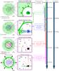 |
Fig. 1 Sketch of the proposed model for the first 40 Myr of evolution of a two-population globular cluster together with the global timeline (top to bottom) and the associated time when the stellar life ends for selected stars on the right. The leftmost column shows the whole cluster. The second column from the left represents a zoom on an FRMS. Four important stages are depicted. First row from top: first a mass-segregated star cluster is formed with all FRMS inside the half-mass radius (dashed line) and with the initial gas (light pistachio-green shade) remaining after the star formation. Each massive star (the blue interior signifies the convective hydrogen burning core, the bright forest-green envelope depicts the convective envelope, which still has the pristine composition at this stage) creates a hot bubble around it. The corresponding wind shell is shown in a darker shade of green than the uncompressed gas. Second row: all hot bubbles connect and create a spongy structure in the centre. At the same time, slow mechanical winds around the FRMS create a disk around them. The outer envelope of the FRMS is now blue to denote that it has been contaminated by hydrogen-burning products. In the interaction between the ejected disc (blue) and the accreting ISM (green), a second generation of chemically different stars is born (blue filled circles). Third row: SNe (red stars with straight lines) fail to eject the gas but create a highly turbulent convection zone. Additional accretion onto the remaining FRMS discs is inhibited. The equatorial ejections also end around this time and the formation of the second-generation stars is completed by about 10 Myr on the global time axis. Bottom row: subsequently, rapid gas expulsion takes place and removes the remaining gas together with the majority of the less tightly bound first-generation stars out of the cluster potential well. Such a rapid gas expulsion is likely to be caused by the activation of black holes by accretion of matter. |
In Krause et al. (2012, Paper I) we showed that gas expulsion via SNe, which has long been the prevailing paradigm to change the GC potential well and induce the loss of first-generation low-mass stars, does not work in GCs. The reason is that while the energy produced by SNe usually exceeds the binding energy, it is not delivered fast enough to avoid the Rayleigh-Taylor instability of the escaping shell. We have also shown that a more powerful event, such as the energy released by accretion onto the dark remnants, may lead to successful gas expulsion. These results suggest three distinct chronological phases in typical GCs: wind bubbles are created during the whole period from about 0 to 8.8 Myr on our global timescale. Core-collapse to black holes and neutron stars occurs from about 3.5 Myr until 35 Myr. Where black holes are formed, the collapse may not be accompanied by a strong or even any momentum ejection. If we therefore consider that only stars with initial masses below 25 M⊙ will give birth to an energetic supernova event, then energy ejection by supernovae will occur only between 8.8 Myr and 35 Myr on the global timescale. Finally, the dark remnants are activated and expel the gas as well as the majority of the first-generation stars.
Here, we explore the implications of these findings for the formation of the second-generation stars in the context of the FRMS scenario and develop a detailed timeline for the first ≈ 40 Myr in the lifetime of a typical GC. We describe the basic model setup in Sect. 2. The wind bubble, supernova, and dark-remnant accretion phases are described in Sects. 3–5. We discuss our findings in Sect. 6 and summarise and conclude in Sect. 7. To describe the sequence of events, we refer to a global timescale throughout this article. The global clock is set to zero at the coeval birth of the first generation of stars.
2. Basic model setup
The model presented here generally follows the ideas outlined in Decressin et al. (2007b, 2010). We consider an initial dense gas cloud of Mtot = 9 × 10⁶ M⊙ with a half-mass radius of r1/2 = 3 pc that forms the first-generation stars with an efficiency of ϵsf = 1/3 and according to a Salpeter IMF for first-generation stars more massive than 0.8 M⊙ and to a log-normal distribution for less massive long-lived stars of first and second generations. The parameters summarised in Table 1 are inferred from N-body simulations that assume a Plummer distribution for the spatial distribution of gas and stars (i.e., the star formation efficiency is similar at all radii; Decressin et al. 2010). For our model cluster, we find about 5700 first-generation massive stars between 25 and 120 M⊙. Mass segregation leads to all massive stars to be located within r1/2. We used the stellar evolutionary models of FRMS at subsolar metallicity (Z = 0.0005, [Fe/H] ≂ −1.5) presented by Decressin et al. (2007b). From these models, we extracted the relevant wind parameters, summarised in Table 2. Decressin et al. (2010) used these parameters to describe the GC NGC 6752 with a present-day mass of 3 × 10⁵ M⊙, assuming complete recycling of the slow wind released by FRMS and dilution with pristine gas to reproduce the observed Li-Na anti-correlation. For this set-up, we now explore the different phases in detail. A sketch of the model is provided in Fig. 1.
Parameters of the model cluster.
3. Hot wind-bubbles
We now argue (Sect. 3.1) that during the first few Myr of the GC, before the first type II SNe, the fast radiative winds of the massive stars will create large bubbles that will probably also overlap, but they will probably not unite into a single superbubble and will not lift any important amount of gas out of the GC. This situation is depicted in Fig. 1 (second row from top). We also show that during this wind-bubble phase (and also during the supernova phase), no stars should form in the normal way (Sect. 3.2), that the equatorial ejections of the FRMS establish a decretion disc close to the FRMS (Sect. 3.3), and that accretion may be re-established in the shadow of these decretion discs (Sect. 3.4). The inner decretion disc and the outer accretion disc merge on the viscous timescale (Sect. 3.5), and finally the second-generation stars form in the merged discs (Sect. 3.6).
Properties of low-metallicity fast-rotating massive stars.
3.1. Bubble expansion
To see that the wind bubbles cannot unite into a single superbubble and that they will also not lift much gas out of the GC’s potential well, we consider the energy budget in the cluster.Freyer et al. (2003) derived that the mechanical power output of a star dominates the effect on the intra-cluster medium (ICM) rather than the effect of ionisation. The power output of the fast winds of a FRMS with a given mass M between 40 M⊙ and 120 M⊙ may be approximated by  (1)This power law follows from interpolating the values in Table 2. With a Salpeter IMF, the total wind output, which is dominated by the most massive stars, integrates to Q0,tot = 2 × 1039 erg s-1 = 6 × 1052 erg Myr-1.
How much of this energy is used to extend the bubbles and not lost to radiation? Freyer et al. (2003) derived that for a background density of 20 cm-3, much lower than the density expected in a young GC, about 90 per cent of this power is radiated away, and thus the energy efficiency is only 10%. If the bubble were to remain self-similar, a greater energy efficiency around 70% would be expected (Weaver et al. 1977; Freyer et al. 2003). Krause et al. (2013) studied the energy efficiency of merging wind bubbles, and found that there is no additional effect from bubble merging for small separations, and that the efficiency factor remains unchanged. We expect that in the dense environment of a forming GC radiation losses may increase and the efficiency of energy transfer may be reduced below the value of Freyer et al. (2003). On the other hand, the optical depth is higher, and more of the radiation energy may be captured by the gas. In the following, we adopt η = 0.1 as a working hypothesis for the energy efficiency, but the conclusions are unchanged if η = 0.01.
The gravitational binding energy of the gas is Egrav = 0.4(1 − ϵsf)GM2/R ≈ 6 × 1053 erg (Baumgardt et al. 2008). The combined wind power of all massive stars amounts to ηQ0,tot = 6 × 1051(η/0.1) erg Myr-1. Thus, it is not possible for the stellar winds to lift any noteworthy amount of gas out of the GC on a relevant timescale.
On the other hand, we may integrate the volume fraction occupied by the wind bubbles by integrating the standard wind bubble volume  over the IMF. The bubble radius rbubble at time t is given by
  (2)where α ≈ 0.8 for the self-similar expansion (Weaver et al. 1977), and the not necessarily self-similar thin shell approximation alike (Krause 2003). The average gas density in our model cluster is ρ0 = 106mp cm-3. We include the efficiency factor η in Eq. (2) because the expansion law in this form is consistent with the sizes of observed wind bubbles (e.g. Oey & García-Segura 2004,and references therein). We show the volume fraction occupied by hot bubbles in Fig. 2. The hot wind-bubbles fill the GC very quickly on a timescale of 0.1 Myr.
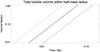 |
Fig. 2 Combined volume of the wind bubbles of all 5700 massive stars (M > 25 M⊙) in our model cluster as a fraction of the half-mass radius. The solid (dotted, dashed) line is for an energy injection efficiency of η = 0.1 (1, 0.01). |
Thus, while the wind bubbles are unable to lift the gas out of the potential well of the GC, they are nevertheless able to quickly fill the entire volume within the half-mass radius, regardless of what we assume in detail for the energy efficiency. It follows that the bulk of the cluster gas is compressed into thin filaments or sheets, while most of the volume is occupied by hot wind-bubbles. Bubbles from stars of different masses in general do not have the same pressure, and thus many individual interfaces may be expected to be swept away and pushed against some other bubble walls (van Marle et al. 2012; Krause et al. 2013). Accordingly, it is clear that some individual bubbles will unite to form larger bubbles, but there will be no single superbubble, which would imply significant lift-up of gas out of the potential well of the GC.
3.2. Lyman-Werner flux
Conroy & Spergel (2011) highlighted that during the main-sequence phase of the massive stars, the Lyman-Werner flux (912 Å–1100 Å) is so high that molecular hydrogen is dissociated throughout the cluster, and no stars may form in the usual way during this time. We repeat their analysis here, but with the numbers from the FRMS models of Decressin et al. (2007b). We calculated the Lyman-Werner flux from these models and included it in Table 2. A reasonable fit to the photon fluxes, which are roughly constant during the main sequence, as a function of mass of the parent star is  (3)Conroy & Spergel (2011) estimate the radius of the photo-dissociation region to
 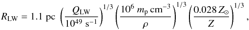 (4)adapted to the metallicity of our model stars. Thus, one 120 M⊙ star is able to photo-dissociate a large fraction of our model GC. Integrating over a Salpeter IMF gives the factor fLW, which describes how many times the GC volume could be photo-dissociated by the ultraviolet radiation:
 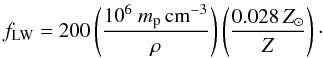 (5)This means that even if the metallicity or the gas density were higher by one or even two orders of magnitude, the gas would still be fully photodissociated.
In addition to the effects of dust considered in the above analysis, molecular hydrogen may also form via electrons, which first combine with neutral hydrogen to H−. H2 is then formed by the reaction:  (6)Regions where both electrons and neutral hydrogen atoms are abundant are rare. Ricotti et al. (2001) showed that the interface between an H II region and a neutral region is such a promising place, and that molecular hydrogen may form there in a narrow layer. They found a strong dependence on the input spectrum and a maximum column density of log (NH2/cm-2) = 14–15 of molecular hydrogen formed in this layer. The corresponding gas mass itself would be too small to form any significant amount of stars in the GC context. However, Ricotti et al. (2001) also showed that the column is sufficient for some Lyman-Werner bands to become optically thick. Hence, these layers might in principal shield pockets of dense gas from photo-dissociation. Quantitatively, Ricotti et al. (2001) find that the radius of photo-dissociation regions may be reduced by a factor of 1.5, corresponding to a factor of 3.4 in volume. This would be too small to be significant, however, since we have shown above that there are enough photons to ionise the entire volume about 200 times. This crude order of magnitude estimate stands up to recent three-dimensional radiative transfer simulations: Wolcott-Green et al. (2011) showed that passage through molecular hydrogen with a column density of NH2 ≡ 5x × 1014 cm-2 attenuates the Lyman-Werner flux (within an accuracy of 15 per cent) by the factor
 ![Mathematical equation: \begin{eqnarray} f_\mathrm{shield}(N_{\mathrm{H}_2},T) &=& \nonumber \frac{0.965}{(1+x/b_5)^{1.1}} + \frac{0.035}{(1+x)^{0.5}} \\ & &\times \exp \left[ -8.5\times 10^{-4} (1+x)^{0.5}\right]\, , \end{eqnarray}](/articles/aa/full_html/2013/04/aa20694-12/aa20694-12-eq72.png) (7)where b5 ≡ b/(km s-1) is the Doppler-broadening parameter. If thermal broadening dominates, b5 should be around or below unity. If there is substantial velocity shear in the filaments, it might be higher. A reduction of the Lyman-Werner flux by a factor of 200 (to bring the photo-dissociated volume fraction below unity) is reached at log (NH2/cm-2) = 17 (16,18) for log (b5/km s-1) = 0 (–1,1). This confirms that the aforementioned layers at the interface of ionised and neutral regions with log (NH2/cm-2) = 14–15 would not provide a significant optical depth that could significantly alter the conclusion above. A combination of this effect with strong dust absorption might perhaps allow for some molecular hydrogen in the densest parts of the ICM. However, the question would remain why these dense pockets would not have formed stars right away.
(7)where b5 ≡ b/(km s-1) is the Doppler-broadening parameter. If thermal broadening dominates, b5 should be around or below unity. If there is substantial velocity shear in the filaments, it might be higher. A reduction of the Lyman-Werner flux by a factor of 200 (to bring the photo-dissociated volume fraction below unity) is reached at log (NH2/cm-2) = 17 (16,18) for log (b5/km s-1) = 0 (–1,1). This confirms that the aforementioned layers at the interface of ionised and neutral regions with log (NH2/cm-2) = 14–15 would not provide a significant optical depth that could significantly alter the conclusion above. A combination of this effect with strong dust absorption might perhaps allow for some molecular hydrogen in the densest parts of the ICM. However, the question would remain why these dense pockets would not have formed stars right away.
We therefore confirm the result of Conroy & Spergel (2011) with the star models of Decressin et al. (2007b) that molecular hydrogen is no longer present in significant amounts in the GC as soon as the massive stars reach the main sequence. From the similarity of the numbers for our star models at a metallicity of Z = 0.03 Z⊙, with their case for Z = 0.1 Z⊙, it follows that this result should not depend very much on the exact metallicity of the GC. Thus, at least low-mass stars do not form in the “classical” way during this time, because the gas is efficiently kept at ≈ 100 K. We note that this remains true throughout the wind-bubble and the supernova phase.
3.3. Equatorial mass ejections
Angular momentum transfer within the FRMS causes episodic equatorial mass ejections of gas enriched by hydrogen-burning products when the star reaches break-up, forming decretion discs (Decressin et al. 2007b; Krtička et al. 2011) around the stars. This process is analogous to the equatorial mass loss in Be-type stars (e.g. Rivinius et al. 2001; Townsend et al. 2004; Haubois et al. 2012). In FRMS, the total amount of mass lost by this process is rather high, and it is hardly plausible that the ejected material may immediately leave the vicinity of the star: to lift the material out of the gravitational potential of the parent star, an energy supply at a rate of GMṀ/(2Rdd) is required if the decretion disc is first established at a characteristic radius Rdd after being ejected. The factor of two in the denominator takes into account the rotational energy of the gas. This material leaves the star because of supercritical rotation. Therefore, it is reasonable to assume that it will be ejected with the necessary angular momentum to be stable just outside the star. As an estimate, we take Rdd to be three photospheric radii (compare Table 2). For the 40 (60,120) M⊙ star, we find a required energy injection rate of 1.4 (1.7, 13) × 1036 erg/s. The power in the fast, radiative wind is a few to up to a factor of ten times less2. The equatorial ejections should cover only a small part of the solid angle (Krtička et al. 2011), whereas at the same time the radiation of fast-rotating stars is concentrated towards the poles (e.g. Maeder & Meynet 2012). In light of these considerations, it seems highly implausible that a significant part of the disc should leave the immediate vicinity of the parent star, although there may likely be some moderate mass loss through photo-evaporation, and the disc may spread out somewhat through angular momentum transfer (Krtička et al. 2011).
The mass lost by the equatorial mechanism averaged over the total ejection time, which includes the main sequence and the luminous blue variable stages, can be fitted by the formula: ![Mathematical equation: \begin{equation} \label{eq:eqej} \dot{M}_\mathrm{eq}= \left[9 \left(\frac{M}{60~M_\odot}\right) -4.8 \right] ~M_\odot /\mathrm{Myr} \end{equation}](/articles/aa/full_html/2013/04/aa20694-12/aa20694-12-eq82.png) (8)for stars with mass M > 32 M⊙. The latter limit is simply due to the zero-point in Eq. (8). This is quite realistic, however, because the 40 M⊙ model still has a high equatorial mass loss rate, whereas in the 25 M⊙ model it is close to zero.
(8)for stars with mass M > 32 M⊙. The latter limit is simply due to the zero-point in Eq. (8). This is quite realistic, however, because the 40 M⊙ model still has a high equatorial mass loss rate, whereas in the 25 M⊙ model it is close to zero.
3.4. Accretion onto the discs around the massive stars
3.4.1. The discs persist around the FRMS
The off-time between any two equatorial mass ejections is a few times the on-time (Table 2). Also the radiative energy accumulated in the off-time, when no new mass is ejected equatorially, but the radiation pressure keeps pushing, is likely not sufficient to unbind the entire disc from the parent star. Another process to consider are close encounters of other massive stars, which could in principle unbind a disc (Clarke & Pringle 1993; Hall et al. 1996). In the unfavourable prograde encounter, the disc would be stripped to about half the periastron radius. The timescale for a given massive star to have a close encounter with another massive star is given by (nσv)-1, where  pc-3 is the density of massive stars, σ = π(2Rdd)2 is the characteristic cross section of the accretion disc, and v ≈ 100 km s-1 is the typical velocity of the massive stars. Using any of the values for the disc radii discussed above, the encounter timescale turns out to be much larger than the Hubble time. Thus, the discs cannot be tidally stripped. Moreover, because of small cross section of the FRMS discs, ram-pressure stripping is equally ineffective.
3.4.2. Re-establishment of accretion
The shielding from the parent star radiation should allow a re-establishing of the accretion flow that provides pristine gas (Fig. 1,second row from top, right). The Bondi accretion rate should set an upper limit for the mass accumulation in the disc. With the sound speed for an atomic gas consisting of 90 per cent hydrogen and 10 per cent helium by number,  , and a solid angle fraction fsd of the disc available for accretion, the Bondi accretion rate is (Frank et al. 2002)
  (9)This accretion rate is most likely not sustained throughout the lifetime of the massive stars. One reason is that the dense gas should be compressed into filaments at this time (compare above), so that accretion may only take place when the star passes through a filament. We show below that for suitable orbit parameters, the total path an FRMS traverses at low velocities is long compared to the typical bubble size. Since the dependence on the density is linear, we therefore do not need to take this into account for the present discussion, because a reduced accretion rate in voids would be compensated for by an increased accretion rate in the filaments.
3.4.3. Accretion suppressed through high stellar velocities
If a star moves with a velocity v relative to the local ICM, the accretion rate is reduced by a factor (v/cs)3 (Bondi & Hoyle 1944). For typical virial velocities of about 100 km s-1, this would lead to a suppression of about six orders of magnitude. Orbits of stars in GCs are not expected to be circular, and therefore the accretion rate is a strong function of the position of a given star along its orbit: It accretes more strongly when the velocity relative to the ICM is low, i.e. near the outer turning point and when at the same time it passes through a filament.
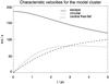 |
Fig. 3 Characteristic velocities for the model GC (compare Table 1) as a function of radius. The solid line shows the local escape velocity. The dotted line is for the circular velocity. The dashed line shows the velocity a star would have obtained in the centre if it were to start at rest at a given radius r. |
We now estimate the time-averaged accretion rate for a given star. In a spherical potential, the orbits are generally expected to be of the rosette type (Binney & Tremaine 2008), with many of the stars having only slightly negative total energies. Adapted to our model cluster, many of the massive stars will have just enough energy to reach the core radius at their outer turning points. As can be seen from Fig. 3, the circular velocities at the core radius (2.3 pc) are around 80 km s-1. If the stars were to have no angular momentum, they would reach a similar velocity after a free fall to the centre from this position. Consequently, velocities around 1 km s-1, which are necessary for efficient accretion, can only be reached for very eccentric orbits and only near their outer turning points.
For this estimate, we approximate the orbits by ellipses. The radius r as a function of azimuth φ is then given by  (10)with the eccentricity e and the orbital size parameter p. The orbital velocity follows by differentiation and can be expressed as
  (11)where
  with the semi-major axis a. Instead of the eccentricity, we use in the following the ratio of the velocity at the outer turning point to the circular velocity at this location as parameter. It is given by
  . The orbit-averaged Bondi accretion rate may then be found by integrating Eq. (9) over the appropriate number of orbits, n, multiplied by the suppression factor, (cs/ve)3, and dividing by n times the orbital period T:
 ![Mathematical equation: \begin{equation} \label{eq:mdotav} \langle{\dot{M}}_\mathrm{Bondi}\rangle =\dot{M}_\mathrm{Bondi} \frac{1}{nT}\int_0^{nT}\left[\mathrm{min}\left(1,\frac{c_\mathrm{s}}{v_e}\right)\right]^3 \mathrm{d}t . \end{equation}](/articles/aa/full_html/2013/04/aa20694-12/aa20694-12-eq105.png) (12)
(12)
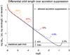 |
Fig. 4 Differential path length over accretion suppression factor f = ⟨ ṀBondi ⟩ /ṀBondi. The five curves labelled by their respective vaz,0/vcirc-value show the path length in parsec that a star spends at a given accretion suppression factor f per orbital period and per decade in log (f). The range of f-values that our model requires is given to the right of the solid vertical bar. The horizontal dotted lines show the limiting path length for statistically uniform accretion. The plot shows that the accumulated path length is sufficient for uniform accretion for all orbits with vaz,0/vcirc ≳ 3%. For orbits with lower values of vaz,0/vcirc, accretion varies strongly from star to star, and the average value shown in Fig. 5 would only apply to the ensemble. The plot also shows, that for all orbits with vaz,0/vcirc < 10% there is always a basic amount of gas that is uniformly accreted onto each FRMS disc. This amount is sufficient for our model. The part of the accreted gas that varies from star to star is only added to this basic amount. See Sect. 3.4.3 for details. |
We recall here that ṀBondi depends on density and temperature. We excluded this from the integral in Eq. (12), because the changes in density along the path of a given star – due to filaments and voids – are not correlated to the changes in velocity. Again, since the Bondi accretion rate is linear in the density, we can use the average value for the density as long as we ascertain that the total path traversed while the velocity of the star is low (the contribution to the integral is negligible otherwise) is long compared to the average bubble diameter. This is indeed the case for an interesting part of the parameter space in vaz,0/vcirc: We parametrise the accretion suppression by f = ⟨ ṀBondi ⟩ /ṀBondi and show the path-length per orbit per decade of log (f) in Fig. 4. The orbital period for stars whose outer turning point is near the core radius is 0.16 Myr for all eccentricities. The minimum accretion time is given by the equatorial ejection phase of the 120 M⊙ star, 2.45 Myr. The maximum accretion time would be 4.6 Myr, which would correspond to the 40 M⊙ star and the case when the massive stars turn into black holes without energetic SNe. Hence, the FRMS complete 15 to 29 orbits in the GC during the time when they have equatorial ejections. To accumulate a total path at low velocity of a bubble diameter, they must therefore spend at least 0.008 pc or, respectively, 0.015 pc at low velocities, per orbit. These two limits are shown as dotted horizontal lines in Fig. 4. A vertical solid line marks the minimum accretion rate we must demand to explain the relative contributions of pristine and ejected gas in the currently observed GC stars. It can be seen that for low values of vaz,0/vcirc, the differential path length distribution is well described by a power law, 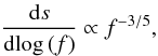 with an upturn at high values of log (f). Figure 4 shows that the accumulated path is generally above the statistical limit for vaz,0/vcirc ≳ 3%. For such orbits, Eq. (12) is therefore valid for each star. Below this value, Eq. (12) is only valid for an ensemble that is sufficiently large. Figure 4 also shows that for all stars with vaz,0/vcirc < 10%, the integrated path between log (f) = −3.5 and log (f) = −2.5 is always much longer than the statistical path length limit. Therefore, these orbits have a uniform basic accretion rate, which is sufficient in the context of our model. But in addition, there can be a strongly varying component. Within these limitations, we may therefore use Eq. (12) to describe the average accretion rate.
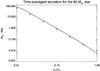 |
Fig. 5 Dependence of the time-averaged accretion rate onto the FRMS as a function of the ratio of the azimuthal velocity at the outer turning point, vaz,0, over the circular velocity, vcirc, for the 60 M⊙ star (see Sect. 3.4 for details). The solid line shows the elliptical approximation. The pluses show the result of a direct orbit-integration in the actual Plummer potential. The two methods agree excellently. |
The orbit-averaged accretion rate for the 60 M⊙ star as a function of vaz,0/vcirc is shown in Fig. 5. We also derived the orbit-averaged accretion rate by direct numerical integration of the orbit in the Plummer potential, which is shown as pluses in the same plot. The good agreement is expected, because the inner regions, where the elliptical approximation is poor, do not contribute much to the average accretion rate. The time averaged accretion rate can be well approximated by 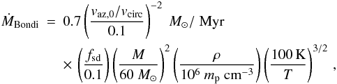 (13)which is fitted to the curve in Fig. 5.
While the characteristic velocity v0 leads to a suppression of the accretion rate by about six orders of magnitude, high orbit-eccentricity may compensate for this to some degree. An accretion rate of about 1.5 M⊙/Myr, which is required to get the correct dilution (i.e., that requested to explain the observed Li-Na anticorrelation) of ejected and pristine gas (compare Eq. (8)), is reached for vaz,0/vcirc = 7% for the 60 M⊙ star. In this case, the gas in the disc around the 60 M⊙ star would consist – on average – of 74% ejected gas from the parent star, and 26% of accreted pristine gas. The accretion rate grows quadratically with the mass of the accreting star, whereas for the equatorial mass ejection rate the dependency is linear. The pristine gas fraction varies therefore with the mass of the parent star. At 60 M⊙ it is close to minimal, for 40 (120) M⊙ it rises to 35% (31%), assuming again vaz,0/vcirc = 7%, We discuss this in more detail in Sect. 3.6.2.
3.5. Viscous merging of accretion and decretion discs
Because of the angular momentum that is likely present in the gas, it will settle into the disc at some radius r, which is likely large compared to the typical locus of the equatorial stellar ejecta. Viscous processes are then responsible for transporting the material within the accretion disc. For a steady, thin, Keplerian disc, the viscous timescale is given by (Frank et al. 2002, p. 88) ![Mathematical equation: \begin{eqnarray} \label{eq:visc} t_\mathrm{visc}&\!=\!&\nonumber \frac{\sqrt{GMr}}{\alpha c_\mathrm{s}^2} \\[-2mm] &\!=\!& 1.6\,\mathrm{Myr} \left(\frac{M}{60~M_\odot}\right)^{1/2} \left(\frac{c_\mathrm{s}}{1\, \mathrm{km\,s}^{-1}}\right)^{-2} \left(\frac{\alpha}{0.1}\right) \left(\frac{r}{0.1 \,\mathrm{pc}}\right)^{1/2},~~ \end{eqnarray}](/articles/aa/full_html/2013/04/aa20694-12/aa20694-12-eq124.png) (14)where a typical value for α is 0.1, and we assumed a radius r of the order of the average distance between massive stars.
(14)where a typical value for α is 0.1, and we assumed a radius r of the order of the average distance between massive stars.
Thus, the viscous evolution of the disc is happening on a similar timescale as the equatorial mass ejection. The re-formed discs near the massive stars are fed by both nuclearly processed gas expelled through equatorial mass ejections, and pristine gas accreted in the shadowed equatorial region. It is therefore plausible that these discs develop a mixture of gas that has overall very similar contributions from pristine and processed components, similar to the composition of the second-generation low-mass stars, which are currently observed in GCs (e.g. Prantzos et al. 2007).
3.6. Star formation in the discs
Discs that are comparable in mass to the central object are known as self-gravitating discs (compare e.g. Sect. 3.1 in the review by Armitage 2011). The Toomre criterion (e.g. Shu 1992) readily shows that the inner discs are expected to be gravitationally unstable 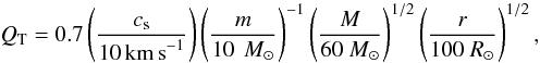 (15)where m is the disc mass, which we assume to be equally distributed within the scale radius r for this estimate. We assumed a higher sound speed in the disc than calculated for the gas on larger scales, because near the massive stars the radiation will heat the discs (compare e.g. Ahmed & Sigut 2012). However, even for a sound speed of 10 km s-1, the inner discs reach the critical mass for gravitational instability on a timescale of 106 years.
3.6.1. Consequences of gravitational instability
Gravitationally stable as well as unstable discs have been studied in the context of planet formation. The latter case is not yet fully understood, however (compare e.g. the review by Kley & Nelson 2012). Spiral density waves with associated torques and strong accretion are a likely outcome. It is therefore possible that some disc material is accreted onto the FRMS, particularly in the “off-phases” of the equatorial ejections. Yet, this material should then also have a high residual angular momentum compared to the gas in the outer regions of the star. Accordingly, the time interval to the next ejection should be shortened. However, the time interval between the ejections is already much shorter than the viscous timescale (Eq. (14)) and the timescale for the disc to become gravitationally unstable. Hence, the disc sees an almost constant flux of material from the star. It is therefore possible that the main sink for the disc mass is the formation of gravitationally bound objects.
Likely, the disc will remain near QT ≈ 1, which implies a disc mass that declines with time, because the FRMS also looses a large fraction of its mass. If the second-generation stars were to form in this way, one would therefore expect that the formation rate of second generation stars, or proto-stars that may continue to accrete for some time, is highest towards the beginning of the equatorial ejections, i.e. about 2–3 Myr after the birth of the first generation of stars (1 Myr until the equatorial ejections also start in the lower mass FRMS, ≈ 1–2 Myr viscous timescale and timescale for the disc to become gravitational unstable). The equatorial ejections cease entirely about 6 Myr after the birth of the first generation of stars, i.e. 2 Myr into the SNe phase, if massive stars explode (compare Sect. 4). We show in Sect. 4.4 that turbulence in this phase stops accretion onto the discs. This effect also keeps the second-generation stars chemically clean from supernova ejecta. Once the discs are no longer fed, they are expected to form their gravitationally bound objects and disappear within at most a few Myr (Haisch et al. 2001). The formation of the second-generation stars is therefore complete at, roughly, 10 Myr after the birth of the first generation of stars.
Consequently, while we are not in a position to add all the details that still need to be worked out in the context of the formation of self gravitating bodies in discs, it appears viable that the second generation of stars forms over a timescale of 6–10 Myr in discs around FRMS (Fig. 1, second row from top).
3.6.2. The distribution of orbit eccentricities and the ratio of pristine-to-processed gas in the second generation stars
We have seen in Sect. 3.4.3 that the amount of gas a given FRMS disc accretes from the ICM strongly depends on the parameter vaz,0/vcirc. The distribution function of vaz,0/vcirc for the sample of FRMS in the cluster will therefore directly determine the distribution of the amounts of accreted ICM to the FRMS discs.
The actual abundance pattern in each second-generation star will not only be determined by the overall ratio of pristine gas accreted from the ICM over ejected gas from the FRMS, however. The abundances in each disc will be also a function of time because of the time dependence of the abundances in the equatorial ejecta (Decressin et al. 2007b). The composition of the equatorial ejecta is first very similar to that of the pristine gas. Eventually, the composition changes and shows increasing signatures of hydrogen burning. Decressin et al. (2007b) have shown that the observed spread in light element abundances may only be obtained if the time variation of the abundances in the ejecta is used. For example, only at late times do we obtain oxygen depletions high enough to be compatible with the oxygen-poor end of the abundance distributions in many GCs (Gratton et al. 2012). If we were to mix all ejecta of a given star into a common reservoir, which would be the disc in our case, the average oxygen depletion would already be insufficient to explain many of the observed second-generation stars. Additional mixing with pristine gas would exacerbate the situation. We therefore require that the star formation in the FRMS discs happens sequentially. This means that for each second-generation star, its formation is complete on a timescale significantly shorter than the lifetime of its parent FRMS disc, so that it may conserve the current abundance pattern of the disc at the time of its formation. This may for example be achieved by migration towards outer orbits, where the gas densities in the discs are low, or through encounters between second-generation stars, which might scatter them out of the disc plane.
A consequence of this way of star formation is that the distribution of abundances will always be continuous. Even in the extreme case when we assume a population of stars with circular orbits, which therefore do not accrete anything from the ICM, together with a population of stars with low eccentricities, which therefore accrete strongly, we would only expect that for the population with a higher ICM accretion, the range of metallicities would be reduced. It is difficult to imagine that this could lead to a double-peaked distribution like the one observed by Marino et al. (2008) in M4. We are able to explain the more uniform distribution found in NGC 1851, however (Lardo et al. 2012). Details of abundance distributions will be the subject of future work.
4. Supernovae
It is widely established that massive stars (M ≳ 25 M⊙) end their lives as black holes (e.g. Fryer 1999). Stars initially less massive than this are expected to produce energetic SNe-events or, possibly, gamma-ray bursts for fast rotators (e.g. Yoon et al. 2006; Dessart et al. 2012). This is much less clear for the more massive stars (e.g. Fryer 1999; Belczynski et al. 2012), which might turn silently into black holes (compare also the discussion in Decressin et al. 2010, and references therein).
This introduces a considerable uncertainty into our model timeline: the 120 M⊙ star would explode at 3.5 Myr, the 25 M⊙ star at 8.8 Myr. The wind-bubble phase ends and the supernova phase begins at some point within this range with the first energetic supernova. In the following we will use the term supernova for simplicity, always subsuming the possibility of gamma-ray bursts.
We first argue that the SNe will likely not significantly alter the picture of the star formation in the FRMS discs (Sect. 4.1). The SNe will cause substantial turbulence in the ICM (Sect. 4.2), which will likely lead to mixing of the SN-ejecta with the cold phase of the ICM (Sect. 4.3). The SN-ejecta may not enter the second-generation stars, however, because on the one hand, the ICM does not form stars in this phase, and on the other hand, the ICM can no longer accrete onto the FRMS discs because of the high gas velocities (Sect. 4.4). From the end stages in the lives of the FRMS onwards, we expect the second-generation stars to be dispersed, first within the half-mass radius, and on the relaxation timescale also throughout the whole cluster (Sect. 4.5).
4.1. Effect of supernovae on the associated star-forming disc
Supernova ejecta are fast and cannot be retained in the gravitational potential of the discs around their parent stars (compare Decressin et al. 2007a,b). Because the disc occupies only a small solid angle, much of the energy will escape into the other directions, especially if the energy release occurs in the form of jets, which might be the case for fast-rotating massive stars (e.g. Bisnovatyi-Kogan & Moiseenko 2008; Takiwaki et al. 2009; Dessart et al. 2012), and ablate only the surface of the disc. At this point (4.5 Myr for the 60 M⊙ star) we might expect that a large fraction of the inner disc gas has already accreted onto the newly formed stars. In this case, some remaining debris might be cleared away by the explosion. Yet, it is also possible that a substantial amount of gas is left. If there were still a substantial amount of gas in the disc, one would expect a compression of the disc and stronger gravitational instability during this phase, similar as in the simulations of Gaibler et al. (2012) for galactic scales.
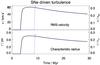 |
Fig. 6 RMS-velocity (upper part) and characteristic radius (lower part) established in the SNe-driven convective phase. The left axis shows km s-1 and pc. The right axis indicates the velocity in units of the central escape velocity and the radius in units of the half-mass radius. The solid black line is for the case when all massive stars produce energetic SNe. The dotted blue line assumes direct black-hole formation without energy release into the ICM for all stars with M > 25 M⊙. The plot shows that in the latter case the onset of turbulence is delayed by 5.3 Myr. See Sect. 4.2 for more details. |
4.2. Effect of supernovae on the general ICM: turbulence
Supernovae are energetic enough to overcome the gravitational potential of the cluster. They are expected to form a superbubble with an expanding shell. As shown in Paper I, such a shell would be quickly destroyed by the Rayleigh-Taylor instability. The situation is similar to the one described by the 2D-axisymmetric simulations of Kritsuk et al. (2001): The fragments of the shell are expected to fall back into the GC, and a convective cooling core is expected to form. Now, the hot high-entropy gas escapes, while cooling shell-fragments are continuously formed at the edges of escaping bubbles, and fall back towards the centre, much like in a boiling pot of water.
We now estimate whether the typical turbulent velocities could lead to a significant increase of the scale height of the gas. We are particularly interested in the cold gas because most of the mass is expected to be in this phase. Hydrodynamic energy transfer is expected between the different gas phases (e.g. Krause & Alexander 2007). In equilibrium, the energy input from SNe should be balanced by radiative losses. But it is not clear that such an equilibrium may be reached: In the simulations of Kritsuk et al. (2001) the convection zone expands slowly, reflecting a steady energy accumulation. Krumholz et al. (2006) summarised simulations of isothermal turbulence and found a decay time of tdis = 0.83λin/vrms. The injection scale in our case is given by the half-mass radius because this is roughly the scale where the shells are destroyed by the Rayleigh-Taylor instability. Following Krumholz et al. (2006), we set the injection wavelength to λin = 4r1/2, because the gas is first in isotropic infall, and also because this is the maximum possible wavelength. The rms-velocity is given by  , because the cold gas is supersonic so that the thermal energy may be neglected. We can thus approximate the change of the energy in the gas by
  (16)Once the rms-velocity is calculated by this approach, the characteristic radius out to which a given gas filament may ascend in the potential of the GC follows from
  (17)where the central escape velocity ve,0 = 183 km s-1 for our model GC. We plot in Fig. 6 the evolution of the rms-velocity and the characteristic radius of the convective flow for the case when the gas would be supported by turbulence alone. Our choice of λin guarantees the lowest possible dissipation rate. The turbulent velocities reached are high compared to normal interstellar medium (ISM) turbulence, about 50 km s-1. Still, this falls short of the escape speed. However, if the gas were to have some other means of support, apart from ram pressure due to turbulence, it would be quite likely that it would still be supported in this other way. Alternative means of support against gravity could be through magnetic fields or to some degree also through radiation pressure (Krumholz & Thompson 2012). If this were the case, our result might also be interpreted in the way that SNe-driven turbulence is unable to increase the scale height of the gas in this phase in any significant way. The characteristic turbulent velocity is mainly determined by the ratio of energy injection to gas mass, and also by the size of the cluster via tdis. Accordingly, because GCs all have a typical radius of a few pc and because the ratio of energy injection to gas mass depends only on the star formation efficiency, which should be always around 1/3 for efficient ejection of the first generation stars (Decressin et al. 2010), we expect that turbulence at 50 km s-1 should be typical for most GCs in this phase. For proto-cluster clouds with initial masses above 106 M⊙, which should be approximately the minimum initial gas mass to form a GC, this is below the escape velocity. Consequently, except for very low mass protocluster clouds with high star formation efficiency, these findings should be generally applicable for all GCs.
4.3. Mixing of supernovae ejecta with pristine gas
Turbulence is considered to be a decisive factor in mixing theories (for a review see Scalo & Elmegreen 2004). Mixing of stellar ejecta into ICM that forms subsequent generations of stars is strongly constrained by observations (e.g. Gratton et al. 2012, and Sect. 1, above). Here, we are interested in an order-of-magnitude estimate and therefore use the mixing length approach. We follow Xie et al. (1995), who applied the mixing length theory to interstellar clouds. Within this framework, the mixing timescale is given by τ ≈ H/vd, where H represents a mean of abundance and density scale heights, and vd is the diffusion velocity, given by vd ≈ K/H. The diffusion coefficient K is simply approximated by the product of the characteristic turbulent velocity, Vt and the mixing length L. We assumed a filament thickness of the order of 0.1 pc in the SNe-driven turbulence phase, and set L = H = 0.1 pc. Thus, the diffusion velocity equals the turbulent one. We have shown above that the expected turbulent velocity in the SNe-driven turbulence phase is approximately 50 km s-1, which therefore would be the characteristic diffusion velocity in the cold gas. The sound speed in the hot component will be higher than this. X-ray observations (e.g. Jaskot et al. 2011) found hot gas temperatures of about 106 K in superbubbles. The sound speed will consequently be several 100 km s-1. Cold gas will therefore more efficiently be mixed into the hot gas than vice versa. Using these assumptions, the mixing timescale is given by  (18)This is to be compared to the dynamical timescale, i.e. the time needed by bubbles enriched with fast winds and SNe ejecta to escape the GC. At times when the GC is highly turbulent, the dynamical timescale is given by
 ![Mathematical equation: \begin{eqnarray} \tau_\mathrm{dyn,t}&=&r_{1/2}/V_\mathrm{t} \nonumber \\[-2mm] &\approx& 60\,000\, \mathrm{yrs} \left(\frac{r_{1/2}}{3 \, \mathrm{pc}}\right) \left(\frac{V_\mathrm{t}}{50 \, \mathrm{km\,s^{-1}}}\right)^{-1}\cdot \end{eqnarray}](/articles/aa/full_html/2013/04/aa20694-12/aa20694-12-eq150.png) (19)When the turbulent velocities are low, the gravitational acceleration of the cold gas, which needs to refill the bubble volume, is the limiting factor. Therefore, the Rayleigh-Taylor timescale sets the minimum for the dynamical timescale:
(19)When the turbulent velocities are low, the gravitational acceleration of the cold gas, which needs to refill the bubble volume, is the limiting factor. Therefore, the Rayleigh-Taylor timescale sets the minimum for the dynamical timescale:  (20)where we have scaled the gravitational acceleration g to the average value within the half-mass radius for our model cluster. Thus, the dynamical timescale is always around 60 000 yr.
This means that in the supernova phase we expect the SNe ejecta to mix with the cold gas phase of the ICM, because of fast turbulent mixing. On the other hand, without an efficient driver, any turbulence should decay quickly and the gas velocities are expected to be of the order of the sound speed, which is expected to be about 1 km s-1 (compare Sect. 3.4). The mixing timescale therefore increases to about 100 000 yr, almost twice the dynamical timescale. Hence, we expect no significant mixing in the wind phase before the onset of the SNe.
The problem of turbulent mixing in the ISM cannot be regarded as settled yet. De Avillez & Mac Low (2002) found in hydrodynamic simulations of SNe-driven turbulence in the Milky Way disc diffusion coefficients that are one to two orders of magnitude smaller than in the mixing length approach. Correspondingly, the mixing timescales we gave above would underestimate the true timescales by one or even two orders of magnitude. While an increase of one order of magnitude would not change our result, two orders of magnitude would mean that no significant mixing would occur in the SNe-driven turbulence phase either.
It has been suggested that stars with masses above 25 M⊙ might not form SNe, but would instead collapse to a black hole without noteworthy energy release (compare above). This would delay the onset of strong turbulence until about 8.8 Myr after the birth of the first-generation stars, the time when the 25 M⊙ stars would explode. The FRMS could in this case accrete from the ICM up to this point. The lack of turbulence would also prevent mixing, so that the stellar ejecta carried by the fast radiative winds of the more massive stars at this time, which carry He-burning products that are not found in the second-generation stars, cannot enter the FRMS-discs. The same argument applies for the end of the wind-bubble phase for the case when the high-mass FRMS do develop SNe.
4.4. Effect of turbulence on accretion
As discussed in Sect. 3.4, accretion is significantly suppressed if the relative velocities between the accreting objects and the accreted gas are high. This is the case for the SNe phase, because the typical gas velocities are around 50 km s-1. Thus, accretion on to the FRMS discs can occur only during the first few Myr (4 to 9 Myr, depending on the mass limit for energetic SNe events) after the birth of the first generation of stars, before the supernova phase. The associated smaller amount of accreted gas may be compensated for by a slight increase of the orbital eccentricities of the FRMS, however (Sect. 3.4). We have shown in Sect. 3.6 that the FRMS discs have disappeared long before the end of the SNe phase. Once a given FRMS has exploded as a supernova, there is therefore at most a short period of activity, and the dark remnants then remain inactive until the last SN has exploded.
4.5. Dispersal of the second-generation stars
The FRMS loose about half of their mass through equatorial ejections loaded with hydrogen-burning products during the main sequence and the luminous-blue-variable stage, and this is the main mass loss channel in this early phase. We expect that towards its end, each FRMS disc has about the same mass as the FRMS, perhaps even slightly more. A considerable fraction of the disc mass should have been used up to form the second-generation stars. Thus, even towards the end of the equatorial ejections, it is expected that gravitational interactions lead to migration of the second-generation stars in the discs, and quite possibly also to some ejections from the discs.
From the end of the equatorial ejection phase, the FRMS continue to loose mass through fast radiative winds and perhaps eventual SNe ejections. The final dark remnants might then have only about ten per cent of the mass that the FRMS had at the end of the equatorial ejection phase. Consequently, the gravitational binding energy, which is to first order simply proportional to the square of the total mass, would have decreased by a factor of a few. Virial equilibrium at the end of the equatorial ejection phase demands that the kinetic energy is half of the binding energy. Therefore, after an SN-ejection, the total energy of the system would be positive. Even without SN-ejection, the mass loss of the FRMS is considerable after the equatorial ejections have ceased. Consequently, the second-generation star orbits widen. This increases the cross sections for collisions. Most of the second-generation stars may be lost from the parent star, but would remain centrally concentrated within the half-mass radius, similar to the FRMS and the dark remnants (compare Fig. 1). The mixing of the first- and second-generation stars through two-body relaxation effects has been studied in detail by Decressin et al. (2008). They showed that the two stellar populations need two relaxation timescales to mix, which corresponds to about 2.8 Gyr, from their Eq. (1). Therefore, there is not enough time for the second-generation stars to spread across the cluster before the majority of the first-generation stars are lost from the cluster during the gas expulsion phase (Sect. 5). But it also appears to be quite possible that the dark remnants retain some of the second-generation stars, which might subsequently form X-ray binaries. X-ray binaries are known to occur in GCs (e.g. Barnard et al. 2012; Barret 2012; Stacey et al. 2012).
5. Accretion onto the dark remnants
After the last type II SNe has exploded, roughly 35 Myr after the formation of the first-generation of stars, turbulence abates. With the formula given in Sect. 4.2, the decay time is given by 0.2 Myr/v50, where v50 is the rms-velocity in units of 50 km s-1.
In principle, black holes and neutron stars may receive natal kicks as strong as ≈ 400 km s-1 (Repetto et al. 2012), fast enough for them to escape from any given GC. However, many neutron stars are observed in GCs (e.g. Barnard et al. 2012; Barret 2012; Stacey et al. 2012). The recent detection of two black holes in the Milky Way GC M 22 (Strader et al. 2012) has called into question whether all black holes receive strong natal kicks. Especially if black holes form directly without SN-ejection, no significant natal kicks are expected. In the following, we therefore assume that the dark remnants have the same orbits as the FRMS have had before. Therefore, accretion should again set in. Assuming 1.4 M⊙ for the neutron stars and 3 M⊙ for the stellar-mass black holes and accretion over the full solid angle, Eq. (9) predicts about 10–100 M⊙/Myr. If we assume a similar suppression as in Sect. 3.4, we obtain 0.003–0.03 M⊙/Myr. The dark remnants will start their energy output after about a viscous timescale, which is needed by the gas to approach close enough to their surface, or respectively, the horizon. The viscous timescale is about 1 Myr, according to Eq. (14). Therefore, each dark remnant will receive 0.003–0.03 M⊙ of gas and then be activated. This compares to the Eddington accretion rate of 0.02 MDRM⊙/Myr, where MDR is the mass of the dark remnant in solar masses. This means that once loaded with gas, the dark remnants could be active at the Eddington rate for about 0.1−0.5 Myr (Fig. 1, bottom). We have shown in Paper I that such a sudden onset of accretion on the stellar mass black holes and neutron stars could plausibly release a sufficient amount of energy to eject the ICM in at most 0.06 Myr, corresponding to about half a crossing time. The mass accreted onto the dark remnants is thus plausibly sufficient for this to occur. The expulsion timescale is short enough to remove also the outer first-generation low-mass stars as well, which do not appear in the GCs today. We have also shown that a gradual activation of the dark remnants as they become available, reinforcing the SNe in that phase, is still insufficient to overcome the Rayleigh-Taylor instability. For the efficiency of energy transfer we have adopted in Paper I (20 per cent of the Eddington luminosity), the limiting proto-cluster cloud mass up to which the gas expulsion worked was about 2 × 10⁷ M⊙. This would mean that gas expulsion would work for most of the observed clusters, except for the most massive ones, e.g. ω Centauri and M 22, where also a spread in iron abundances is observed (Gratton et al. 2012, and references therein).The repeated star-bursts expected in this case are similar to the predictions for nuclear star clusters without supermassive black holes by Loose et al. (1982).
For GCs below this mass limit, additional gas accretion events are expected from about 40 Myr after the birth of the first generation stars because of the slow AGB-winds (D’Ercole et al. 2008). Any such event would re-activate the dark-remnants. The accretion rate and the binding energy are approximately linear in the gas density if the stellar potential dominates. Otherwise, the binding energy decreases even more with gas density. Therefore, we again expect quick gas expulsion. This would be similar to the case of super-massive black holes in nuclear star clusters and elliptical galaxies, which may also be activated by AGB-winds (e.g. Gaibler et al. 2005; Davies et al. 2007; Schartmann et al. 2010; Davies et al. 2010). Black-hole feedback may suppress star formation (e.g. Di Matteo et al. 2005).
6. Discussion
6.1. Orbit eccentricities of the FRMS
The weakest point of the presented scenario is perhaps the fine-tuning required for the orbital eccentricities of the FRMS to obtain sufficiently high accretion rates onto the FRMS discs and also onto the dark remnants (Sect. 3.4). We require velocities near the outer turning points of less than about a tenth of the circular velocity there. The former amount to a few km s-1. We highlight in this context that the requirements are the very same as for the dark-remnant accretion, because the FRMS turn into the dark remnants at the end of their lives. If gas expulsion is indeed caused by the dark remnants, as we have proposed in Paper I, then the orbits are also acceptable for accretion onto the FRMS, unless they are significantly affected by the transformation (compare Sect. 5 above).
6.2. Support of the gas and relation to GC formation scenarios
The FRMS orbits will of course be related to the formation of the GC. This is so far unclear, and different scenarios are considered (compare e.g. Harris et al. 1998; Krause 2002; Kravtsov & Gnedin 2005; Gnedin 2011; Gray & Scannapieco 2011; Harris & Harris 2011). In general, one may consider two classes of physical conditions: First, the first-generation stars could be formed while the gas is in free collapse. This is among the scenarios currently discussed for star formation in general (e.g. Zamora-Avilés et al. 2012). Then, by definition, the stars will be born with high radial velocities and much lower azimuthal velocities, roughly as required. The second option is internal support against gravity in the protocluster cloud. Because the decay time for turbulence is short (compare Sect. 4.2) and an unusually high level of turbulence is required (≈ 100 km s-1), it seems unlikely that such a protocluster would be supported by turbulence. If that were the case, the stars would be expected to form with comparable radial and azimuthal velocities, which would be a serious problem for this scenario. Thermal pressure also seems unlikely because the cooling times would be very short. The protocluster cloud could also be supported by magnetic fields. In general ISM simulations, the coldest and hence densest phase is found to be magnetically supported, in contrast to turbulent support for intermediate temperatures (de Avillez & Breitschwerdt 2005). This agrees with observations of molecular clouds (Crutcher 2012). In a magnetically supported protocluster cloud, the stars would lose their magnetic support immediately after formation, and one would also expect highly eccentric orbits.
6.3. Effects of magnetic fields
Magnetic support would mean that the proto-cluster cloud could keep the same scale height as the stars until the gas is expelled from the GC. This would be highly beneficial because in our scenario accretion takes place mainly when the stars are in the vicinity of the core radius. Magnetic fields might also inhibit accretion, however. Cunningham et al. (2012) showed that Bondi accretion from an isothermal, magnetised gas is suppressed by a factor 0.4cs/cA, where cA refers to the Alfvén speed. This may seem moderate compared to the (cs/v)3-factor for bulk motions at velocity v. But to support the protocluster cloud magnetically, this also amounts to two orders of magnitudes, which would significantly restrict the available orbit eccentricities. Ambipolar diffusion should be significant in this context, however, because the majority of the cold gas would be neutral. Furthermore, Cunningham et al. (2012) assumed that the magnetic flux accumulates around the accretor, which is the underlying physical process inhibiting the accretion. In our case, we would expect the flux to be advected into the accretion discs, there to be dissipated by turbulence. Qualitatively, we therefore believe that a magnetically supported protocluster cloud is a viable alternative in the present context. Radiation pressure might also help to support the gas after the first generation massive stars have formed (Krumholz & Thompson 2012).
6.4. Stronger mass segregation as an alternative to supporting the gas on a scale of the half-mass radius
An alternative to supporting the gas on the scale of the half-mass radius would be to assume a stronger concentration of the gas and the massive stars towards the centre of the GC, implying stronger mass segregation: in our model setup (Sect. 5), we specified that the massive stars are confined to the sphere inside the half-mass radius. Leigh et al. (2013) assumed in their model for dark-remnant accretion and dynamical black-hole ejection in GCs a much stronger mass segregation. This might happen if a GC is formed from merging sub-clumps. In this case, strong mass segregation of the stars is expected to arise in about 106 yr (Allison et al. 2010; Girichidis et al. 2012; Pang et al. 2013). Assuming a velocity dispersion inversely proportional to the stellar mass, as in Leigh et al. (2013), would result in our relevant FRMS population having velocities of about the sound speed. In this scenario, the massive stars and the gas could be very much concentrated towards the cluster centre. Hence, accretion would no longer be affected by the orbital parameters because the FRMS velocities would always be low. In addition to the stronger accretion, the formation of the second-generation stars would in this variation of the scenario proceed in almost the same way as in the standard case (Sects. 3.5 and 3.6). The star-forming discs must have some way to prevent complete mixing of the ejected and the accreted gas to explain the most oxygen-poor stars (compare Sect. 3.6.2). The SN-phase would be essentially unaffected, whereas the accretion onto the dark remnants would also be enhanced. The latter might lead to an observationally interesting collective active phase of the order of the viscous timescale, i.e. about 1 Myr.
6.5. Limitations of dark-remnant accretion through local radiative feedback
Radiative feedback has been found to limit accretion onto stellar-mass black holes in spherical and clumpy accretion flows (Milosavljević et al. 2009). This applies to the dark-remnant accretion phase, because we have assumed spherical accretion in Sect. 5. Milosavljević et al. (2009) showed that the average accretion rate may be limited by a value two or three orders of magnitude below the Eddington limit. They cautioned however, that angular momentum, turbulence, and thermodynamic phase segregation might affect the result. They also found that on short timescales the accretion rate may exceed their limit substantially. We require only a very short active phase of the dark remnants to expel the gas (<105 yr). More work is clearly required to settle the case. The strong observational constraints on the present-day gas content of GCs and the Fe-uniformity of the present-day stars put strong constraints on the gas expulsion mechanism (compare Paper I).
6.6. Top-heavy IMF
Gas expulsion could be substantially facilitated by a non-standard, top-heavy IMF. For the model presented in this paper (Sect. 5), we used a normal IMF, following other recent work (e.g. Decressin et al. 2010; D’Ercole et al. 2011). However, the first-generation low-mass stars are of no importance for our scenario. There is even a problem with their ejection, which we have found here not to work with SN-feedback alone (compare Paper I and Sect. 5, above), and which may therefore require the coherent activity of the dark remnants. The ejected low-mass stars might contribute significantly to the stellar population of the Galactic halo (Schaerer & Charbonnel 2011), but there is no strong constraint on how many stars have to escape. The IMF for the first-generation stars might therefore have been top-heavy (e.g. Prantzos & Charbonnel 2006, and references in Sect. 1). This would not necessarily contradict recent work on clusters formed under typical present-day Milky Way conditions (Hennebelle 2012; Krumholz et al. 2012), because the conditions in which the Galactic-halo GCs formed are not known. The central disc in the Milky Way’s nuclear star cluster, a massive and concentrated star cluster similar in this respect to GCs, is an example for observational evidence for a top-heavy IMF (Bartko et al. 2010). A high star-formation efficiency, as often assumed for GCs, is also discussed for this region (e.g. Silk et al. 2012). A top-heavy IMF has been suggested in the context of GCs on the basis of the energy requirements for the gas expulsion (Marks et al. 2012).
In the extreme case, assuming that almost no first-generation low-mass stars form, the initial mass of our model-protocluster cloud (9 × 10⁶ M⊙, Sect. 2) could be reduced by one order of magnitude. Because of the combined effect of lower gas densities and lower stellar velocities, the accretion suppression factor would be constrained to be higher by a factor of a few, moving the vertical line in Fig. 4 to the right. This would narrow the allowed orbital parameters, requiring somewhat higher eccentricities (but see Sect 6.4 for a non-exclusive model variant that has the opposite effect). Depending on the star-formation efficiency and the energy-injection efficiency in the SN-phase, the SNe might already eject the gas. We stress that this refers to the extreme scenario. We have shown in paper I that even tripling the massive stars would not suffice to expel the gas through supernova feedback. The argument is still valid that favourable conditions for accretion onto the FRMS imply subsequent accretion onto the dark remnants. A possibly reduced gas density due to successful SNe-feedback would cause less accretion onto the dark remnants (linear dependency, compare Eq. (9)), but the binding energy would also be reduced. Hence, the dark-remnant feedback would be expected to keep the GC gas-free.
6.7. Comparison to Be-star decretion discs and “first-star” simulations
A key point in our scenario is the formation of the second-generation stars in discs, fed by accretion of pristine gas and equatorial ejections of the FRMS. Such equatorial ejections are known from Be-type stars (e.g. Rivinius et al. 2001). Recently, the spreading out of such discs is also attempted to be understood in terms of viscous evolution (Haubois et al. 2012), similarly to what we propose here for the FRMS discs.
The formation of stars as opposed to planets in circumstellar discs might seem unusual. But, detailed models have recently be computed in the context of the formation of the first massive stars (e.g. Greif et al. 2012), which also may have been very fast rotators (Stacy et al. 2011). For example, Stacy et al. (2012) simulated the formation of a ≈ 30 M⊙ star with radiative feedback. They found that the radiative feedback does not stop the secondary star formation in the accretion disc. During their simulation time of a few 1000 yr, they formed a few proto-stars of sometimes several solar masses. Clark et al. (2011) formed four secondary proto-stars within 110 yr in a similar simulation. Some of these proto-stars may end up in the primary star. Adapted to the FRMS case, this might then lead to a more rapid sequence of ejections. Clearly, many details need to be worked out, some are not comparable (e.g. the first stars are usually assumed to form in dark-matter halos). Still, we believe that these developments are encouraging.
7. Conclusions
Using FRMS data, we have developed a comprehensive scenario for the formation of second-generation GC stars (compare Fig. 1).
The ICM obtains a spongy structure in the wind phase (Fig. 1, second row) due to the space-filling wind bubbles of the massive stars. We confirm the analysis of Conroy and Spergel that the Lyman-Werner photon flux density is sufficiently high for most of the hydrogen molecules to dissociate and no stars may form in the normal way during the wind and the supernova phase.
If the first-generation massive stars have equatorial ejections, however, as expected in the case of fast rotation, we showed that accretion onto their discs resumes in the shadow of the equatorial ejecta. Massive discs are formed fed by FRMS ejecta from the inside and accretion of pristine gas from the outside. Within an order of magnitude estimate, both contributions can be comparable, as required by self-enrichment calculations (Decressin et al. 2007b), if the orbits of the FRMS are sufficiently eccentric. The second-generation stars may then form through gravitational instability in these discs (Fig. 1, second row). This second-generation star formation might continue for a few Myr through the supernova phase, because SNe ejecta are not expected to enter the discs. The increased pressure from the SN may also compress its associated disc such that the last stars in the respective disc form at this occasion. The second-generation stars form sequentially in their parent FRMS discs with the current light element abundances of the respective discs. We propose this as the physical mechanism underlying the detailed abundance calculations of Decressin et al. (2007b). The formation of the second-generation stars is completed at the latest about 10 Myr after the formation of the first generation. The second-generation stars are first dispersed within the half-mass radius, and much later, after the gas expulsion, also throughout the entire GC.
The SNe drive turbulence at about 50 km s-1 (Fig. 1, third row). The remaining gas outside the discs could then mix with the SN ejecta due to turbulence caused by the SN energy. The gas remains bound to the cluster until the SNe have ceased, turbulence has decayed, and the gas can once more accrete suddenly onto the dark remnants. The gas may not accrete onto the FRMS discs before because of the high turbulent velocities. In this way, the second-generation stars are protected from pollution by SN ejecta and He-burning products in general. These findings should hold for all globular clusters, except possibly for those at the low-mass end if their star formation efficiency significantly exceeds 1/3.
In the dark-remnant accretion phase (Fig. 1, bottom), the gas is efficiently expelled through the strong energy release associated with the accretion onto the dark remnants. This happens fast enough so that a large fraction of less tightly bound first-generation stars are also lost.
There are potential problems for the scenario, however. For efficient accretion, the orbits of the massive stars need to be eccentric, with low angular momenta, and velocities near the outer turning points below about 10% of the circular velocity. This may relate to the formation scenario. It would pose a serious difficulty for this model if such low angular momenta could be ruled out observationally and, consequently, stronger mass segregation would have to be assumed (Sect. 6.4). Furthermore, the gas scale height has to be comparable to the core radius, because the main gas accretion would occur near the core radius. The necessary support of the gas against gravity may be due to radiation pressure (Krumholz & Thompson 2012) and magnetic fields; details for this are beyond the scope of this work, however. Stronger mass segregation would again alleviate this problem.
Star formation in discs around massive stars has only recently begun to be explored. While the results from the “first stars” simulations are encouraging, simulations tuned to the specific conditions in FRMS are not yet available.
If for some reason gas expulsion by dark-remnant accretion would fail (Sect. 6.5), all gas should at some point form stars from the quite possibly SN-enriched gas (Sect. 4.3 for mixing uncertainties), unless some other way of gas expulsion would be found. This would conflict with observations, however, except for the rare andmost massive GCs such as ω Centauri and M 22, which exhibit Fe spread.
Dilution of the AGB ejecta with re-collected gas with pristine chemical composition is mandatory since all current AGB models (e.g. Karakas & Lattanzio 2007; Ventura & D’Antona 2009; Siess 2010) predict that O and Na yields should correlate, which is at odds with the observed abundance anti-correlations. Although several scenarios have been proposed, the gathering mechanism of the required pristine matter is still uncertain (for discussion see D’Ercole et al. 2010, 2011).
Our wind power Q0 refers to the terminal wind power of the fast, radiatively driven wind, but the additional power required to lift the material ejected into this wind out of the gravitational potential is less than 50 per cent of Q0.
Acknowledgments
We thank the referee, Volker Bromm, for very useful comments that helped to improve the manuscript. We also gratefully acknowledge discussions with Mordecai-Mark Mac Low. This research was supported by the cluster of excellence “Origin and Structure of the Universe” (http://www.universe-cluster.de) and the ESF EUROCORES Programme “Origin of the Elements and Nuclear History of the Universe” (grants 189 and 190). C.C. and T.D. also acknowledge financial support from the Swiss National Science Foundation (FNS) and the French Programme National de Physique Stellaire (PNPS) of CNRS/INSU.
References
- Ahmed, A., & Sigut, T. A. A. 2012, ApJ, 744, 191 [NASA ADS] [CrossRef] [Google Scholar]
- Allison, R. J., Goodwin, S. P., Parker, R. J., Portegies Zwart, S. F., & de Grijs, R. 2010, MNRAS, 407, 1098 [Google Scholar]
- Armitage, P. J. 2011, ARA&A, 49, 195 [NASA ADS] [CrossRef] [EDP Sciences] [Google Scholar]
- Barnard, R., Garcia, M., & Murray, S. S. 2012, ApJ, 757, 40 [NASA ADS] [CrossRef] [Google Scholar]
- Barret, D. 2012, ApJ, 753, 84 [NASA ADS] [CrossRef] [Google Scholar]
- Bartko, H., Martins, F., Trippe, S., et al. 2010, ApJ, 708, 834 [NASA ADS] [CrossRef] [Google Scholar]
- Baumgardt, H., Kroupa, P., & Parmentier, G. 2008, MNRAS, 384, 1231 [NASA ADS] [CrossRef] [Google Scholar]
- Bekki, K., & Norris, J. E. 2006, ApJ, 637, L109 [NASA ADS] [CrossRef] [Google Scholar]
- Bekki, K., Campbell, S. W., Lattanzio, J. C., & Norris, J. E. 2007, MNRAS, 377, 335 [NASA ADS] [CrossRef] [Google Scholar]
- Belczynski, K., Wiktorowicz, G., Fryer, C. L., Holz, D. E., & Kalogera, V. 2012, ApJ, 757, 91 [NASA ADS] [CrossRef] [Google Scholar]
- Binney, J., & Tremaine, S. 2008, Galactic Dynamics: Second Edition (Princeton University Press) [Google Scholar]
- Bisnovatyi-Kogan, G. S., & Moiseenko, S. G. 2008, Prog. Theor. Phys. Supp., 172, 145 [NASA ADS] [CrossRef] [Google Scholar]
- Bondi, H., & Hoyle, F. 1944, MNRAS, 104, 273 [NASA ADS] [CrossRef] [Google Scholar]
- Carretta, E., Bragaglia, A., Gratton, R. G., et al. 2009, A&A, 505, 117 [NASA ADS] [CrossRef] [EDP Sciences] [Google Scholar]
- Charbonnel, C. 2010, in IAU Symp. 266, eds. R. de Grijs, & J. R. D. Lépine, 131 [Google Scholar]
- Clark, P. C., Glover, S. C. O., Smith, R. J., et al. 2011, Science, 331, 1040 [NASA ADS] [CrossRef] [PubMed] [Google Scholar]
- Clarke, C. J., & Pringle, J. E. 1993, MNRAS, 261, 190 [NASA ADS] [CrossRef] [Google Scholar]
- Conroy, C., & Spergel, D. N. 2011, ApJ, 726, 36 [NASA ADS] [CrossRef] [Google Scholar]
- Crutcher, R. M. 2012, ARA&A, 50, 29 [NASA ADS] [CrossRef] [Google Scholar]
- Cunningham, A. J., McKee, C. F., Klein, R. I., Krumholz, M. R., & Teyssier, R. 2012, ApJ, 744, 185 [NASA ADS] [CrossRef] [Google Scholar]
- D’Antona, F., & Caloi, V. 2004, ApJ, 611, 871 [NASA ADS] [CrossRef] [Google Scholar]
- Davies, R. I., Mueller Sánchez, F., Genzel, R., et al. 2007, ApJ, 671, 1388 [NASA ADS] [CrossRef] [Google Scholar]
- Davies, R. I., Hicks, E., Schartmann, M., et al. 2010, in Co-Evolution of Central Black Holes and Galaxies, eds. B. M. Peterson, R. S. Somerville, & T. Storchi-Bergmann (Cambridge University Press), IAU Symp., 267, 283 [Google Scholar]
- de Avillez, M. A., & Breitschwerdt, D. 2005, A&A, 436, 585 [NASA ADS] [CrossRef] [EDP Sciences] [Google Scholar]
- de Avillez, M. A., & Mac Low, M.-M. 2002, ApJ, 581, 1047 [NASA ADS] [CrossRef] [Google Scholar]
- Decressin, T., Charbonnel, C., & Meynet, G. 2007a, A&A, 475, 859 [NASA ADS] [CrossRef] [EDP Sciences] [Google Scholar]
- Decressin, T., Meynet, G., Charbonnel, C., Prantzos, N., & Ekström, S. 2007b, A&A, 464, 1029 [NASA ADS] [CrossRef] [EDP Sciences] [Google Scholar]
- Decressin, T., Baumgardt, H., & Kroupa, P. 2008, A&A, 492, 101 [NASA ADS] [CrossRef] [EDP Sciences] [Google Scholar]
- Decressin, T., Baumgardt, H., Charbonnel, C., & Kroupa, P. 2010, A&A, 516, A73 [NASA ADS] [CrossRef] [EDP Sciences] [Google Scholar]
- D’Ercole, A., Vesperini, E., D’Antona, F., McMillan, S. L. W., & Recchi, S. 2008, MNRAS, 391, 825 [NASA ADS] [CrossRef] [Google Scholar]
- D’Ercole, A., D’Antona, F., Ventura, P., Vesperini, E., & McMillan, S. L. W. 2010, MNRAS, 407, 854 [NASA ADS] [CrossRef] [MathSciNet] [Google Scholar]
- D’Ercole, A., D’Antona, F., & Vesperini, E. 2011, MNRAS, 415, 1304 [NASA ADS] [CrossRef] [MathSciNet] [Google Scholar]
- D’Ercole, A., D’Antona, F., Carini, R., Vesperini, E., & Ventura, P. 2012, MNRAS, 423, 1521 [NASA ADS] [CrossRef] [Google Scholar]
- Dessart, L., O’Connor, E., & Ott, C. D. 2012, ApJ, 754, 76 [NASA ADS] [CrossRef] [Google Scholar]
- Di Matteo, T., Springel, V., & Hernquist, L. 2005, Nature, 433, 604 [NASA ADS] [CrossRef] [PubMed] [Google Scholar]
- Frank, J., King, A., & Raine, D. J. 2002, Accretion Power in Astrophysics, 3rd edn. (Cambridge University Press) [Google Scholar]
- Fryer, C. L. 1999, ApJ, 522, 413 [NASA ADS] [CrossRef] [Google Scholar]
- Freyer, T., Hensler, G., & Yorke, H. W. 2003, ApJ, 594, 888 [NASA ADS] [CrossRef] [Google Scholar]
- Gaibler, V., Camenzind, M., & Krause, M. 2005, Proc. 1st Arizona/Heidelberg Symposium, The High Redshift Frontier [Google Scholar]
- Gaibler, V., Khochfar, S., Krause, M., & Silk, J. 2012, MNRAS, 425, 438 [NASA ADS] [CrossRef] [Google Scholar]
- Girichidis, P., Federrath, C., Allison, R., Banerjee, R., & Klessen, R. S. 2012, MNRAS, 420, 3264 [NASA ADS] [CrossRef] [Google Scholar]
- Gnedin, O. Y. 2011, in Computational Star Formation, eds. J. Alves, B. G. Elmegreen, J. M. Girart, & V. Trimble (Cambridge University Press), IAU Symp., 270, 381 [Google Scholar]
- Gratton, R., Sneden, C., & Carretta, E. 2004, ARA&A, 42, 385 [NASA ADS] [CrossRef] [Google Scholar]
- Gratton, R. G., Carretta, E., & Bragaglia, A. 2012, A&ARv, 20, 50 [CrossRef] [Google Scholar]
- Gray, W. J., & Scannapieco, E. 2011, ApJ, 742, 100 [NASA ADS] [CrossRef] [Google Scholar]
- Greif, T. H., Bromm, V., Clark, P. C., et al. 2012, MNRAS, 424, 399 [NASA ADS] [CrossRef] [MathSciNet] [Google Scholar]
- Haisch, Jr., K. E.,Lada, E. A., & Lada, C. J. 2001, ApJ, 553, L153 [NASA ADS] [CrossRef] [Google Scholar]
- Hall, S. M., Clarke, C. J., & Pringle, J. E. 1996, MNRAS, 278, 303 [NASA ADS] [Google Scholar]
- Harris, G. L. H., & Harris, W. E. 2011, MNRAS, 410, 2347 [Google Scholar]
- Harris, W. E., Harris, G. L. H., & McLaughlin, D. E. 1998, AJ, 115, 1801 [NASA ADS] [CrossRef] [Google Scholar]
- Haubois, X., Carciofi, A. C., Rivinius, T., Okazaki, A. T., & Bjorkman, J. E. 2012, ApJ, 756, 156 [NASA ADS] [CrossRef] [Google Scholar]
- Hennebelle, P. 2012, A&A, 545, A147 [NASA ADS] [CrossRef] [EDP Sciences] [Google Scholar]
- Jaskot, A. E., Strickland, D. K., Oey, M. S., Chu, Y.-H., & García-Segura, G. 2011, ApJ, 729, 28 [NASA ADS] [CrossRef] [Google Scholar]
- Karakas, A., & Lattanzio, J. C. 2007, PASA, 24, 103 [NASA ADS] [CrossRef] [Google Scholar]
- Kley, W., & Nelson, R. P. 2012, ARA&A, 50, 211 [NASA ADS] [CrossRef] [Google Scholar]
- Krause, M. 2002, A&A, 386, L1 [NASA ADS] [CrossRef] [EDP Sciences] [Google Scholar]
- Krause, M. 2003, A&A, 398, 113 [NASA ADS] [CrossRef] [EDP Sciences] [Google Scholar]
- Krause, M., & Alexander, P. 2007, MNRAS, 376, 465 [NASA ADS] [CrossRef] [Google Scholar]
- Krause, M., Charbonnel, C., Decressin, T., et al. 2012, A&A, 546, L5 [NASA ADS] [CrossRef] [EDP Sciences] [Google Scholar]
- Krause, M., Fierlinger, K., Diehl, R., et al. 2013, A&A, 550, A49 [NASA ADS] [CrossRef] [EDP Sciences] [Google Scholar]
- Kravtsov, A. V., & Gnedin, O. Y. 2005, ApJ, 623, 650 [NASA ADS] [CrossRef] [Google Scholar]
- Kritsuk, A., Plewa, T., & Müller, E. 2001, MNRAS, 326, 11 [NASA ADS] [CrossRef] [Google Scholar]
- Krtička, J., Owocki, S. P., & Meynet, G. 2011, A&A, 527, A84 [NASA ADS] [CrossRef] [EDP Sciences] [Google Scholar]
- Krumholz, M. R., & Thompson, T. A. 2012, ApJ, 760, 155 [NASA ADS] [CrossRef] [Google Scholar]
- Krumholz, M. R., Matzner, C. D., & McKee, C. F. 2006, ApJ, 653, 361 [NASA ADS] [CrossRef] [Google Scholar]
- Krumholz, M. R., Klein, R. I., & McKee, C. F. 2012, ApJ, 754, 71 [NASA ADS] [CrossRef] [Google Scholar]
- Lardo, C., Milone, A. P., Marino, A. F., et al. 2012, A&A, 541, A141 [NASA ADS] [CrossRef] [EDP Sciences] [Google Scholar]
- Leigh, N. W. C., Böker, T., Maccarone, T. J., & Perets, H. B. 2013, MNRAS, 492 [Google Scholar]
- Loose, H. H., Kruegel, E., & Tutukov, A. 1982, A&A, 105, 342 [NASA ADS] [Google Scholar]
- Maeder, A., & Meynet, G. 2012, Rev. Mod. Phys., 84, 25 [NASA ADS] [CrossRef] [Google Scholar]
- Marino, A. F., Villanova, S., Piotto, G., et al. 2008, A&A, 490, 625 [NASA ADS] [CrossRef] [EDP Sciences] [Google Scholar]
- Marks, M., Kroupa, P., Dabringhausen, J., & Pawlowski, M. S. 2012, MNRAS, 422, 2246 [NASA ADS] [CrossRef] [Google Scholar]
- Milosavljević, M., Bromm, V., Couch, S. M., & Oh, S. P. 2009, ApJ, 698, 766 [NASA ADS] [CrossRef] [Google Scholar]
- Oey, M. S., & García-Segura, G. 2004, ApJ, 613, 302 [NASA ADS] [CrossRef] [Google Scholar]
- Pang, X., Grebel, E. K., Allison, R. J., et al. 2013, ApJ, 764, 73 [NASA ADS] [CrossRef] [Google Scholar]
- Piotto, G. 2009, in The Ages of Stars (Cambridge University Press), eds. E. E. Mamajek, D. R. Soderblom, & R. F. G. Wyse, IAU Symp., 258, 233 [Google Scholar]
- Prantzos, N., & Charbonnel, C. 2006, A&A, 458, 135 [NASA ADS] [CrossRef] [EDP Sciences] [Google Scholar]
- Prantzos, N., Charbonnel, C., & Iliadis, C. 2007, A&A, 470, 179 [NASA ADS] [CrossRef] [EDP Sciences] [Google Scholar]
- Repetto, S., Davies, M. B., & Sigurdsson, S. 2012, MNRAS, 425, 2799 [NASA ADS] [CrossRef] [Google Scholar]
- Ricotti, M., Gnedin, N. Y., & Shull, J. M. 2001, ApJ, 560, 580 [NASA ADS] [CrossRef] [Google Scholar]
- Rivinius, T., Baade, D., Štefl, S., & Maintz, M. 2001, A&A, 379, 257 [NASA ADS] [CrossRef] [EDP Sciences] [Google Scholar]
- Scalo, J., & Elmegreen, B. G. 2004, ARA&A, 42, 275 [NASA ADS] [CrossRef] [Google Scholar]
- Schaerer, D., & Charbonnel, C. 2011, MNRAS, 413, 2297 [NASA ADS] [CrossRef] [MathSciNet] [Google Scholar]
- Schartmann, M., Burkert, A., Krause, M., et al. 2010, MNRAS, 403, 1801 [NASA ADS] [CrossRef] [Google Scholar]
- Shu, F. H. 1992, Physics of Astrophysics, Vol. II (Mill Valley, California: University Science Books) [Google Scholar]
- Siess, L. 2010, A&A, 512, A10 [NASA ADS] [CrossRef] [EDP Sciences] [Google Scholar]
- Silk, J., Antonuccio-Delogu, V., Dubois, Y., et al. 2012, A&A, 545, L11 [NASA ADS] [CrossRef] [EDP Sciences] [Google Scholar]
- Stacey, W. S., Heinke, C. O., Cohn, H. N., Lugger, P. M., & Bahramian, A. 2012, ApJ, 751, 62 [NASA ADS] [CrossRef] [Google Scholar]
- Stacy, A., Bromm, V., & Loeb, A. 2011, MNRAS, 413, 543 [NASA ADS] [CrossRef] [Google Scholar]
- Stacy, A., Greif, T. H., & Bromm, V. 2012, MNRAS, 422, 290 [NASA ADS] [CrossRef] [Google Scholar]
- Strader, J., Chomiuk, L., Maccarone, T., Miller-Jones, J., & Seth, A. 2012, Nature, 490, 71 [NASA ADS] [CrossRef] [Google Scholar]
- Takiwaki, T., Kotake, K., & Sato, K. 2009, ApJ, 691, 1360 [NASA ADS] [CrossRef] [Google Scholar]
- Townsend, R. H. D., Owocki, S. P., & Howarth, I. D. 2004, MNRAS, 350, 189 [Google Scholar]
- van Marle, A. J., Meliani, Z., & Marcowith, A. 2012, A&A, 541, L8 [NASA ADS] [CrossRef] [EDP Sciences] [Google Scholar]
- Ventura, P., & D’Antona, F. 2009, A&A, 499, 835 [NASA ADS] [CrossRef] [EDP Sciences] [Google Scholar]
- Weaver, R., McCray, R., Castor, J., Shapiro, P., & Moore, R. 1977, ApJ, 218, 377 [NASA ADS] [CrossRef] [Google Scholar]
- Wolcott-Green, J., Haiman, Z., & Bryan, G. L. 2011, MNRAS, 418, 838 [NASA ADS] [CrossRef] [Google Scholar]
- Xie, T., Allen, M., & Langer, W. D. 1995, ApJ, 440, 674 [NASA ADS] [CrossRef] [Google Scholar]
- Yoon, S.-C., Langer, N., & Norman, C. 2006, A&A, 460, 199 [NASA ADS] [CrossRef] [EDP Sciences] [Google Scholar]
- Zamora-Avilés, M., Vázquez-Semadeni, E., & Colín, P. 2012, ApJ, 751, 77 [NASA ADS] [CrossRef] [Google Scholar]
All Tables
All Figures
|
Fig. 1 Sketch of the proposed model for the first 40 Myr of evolution of a two-population globular cluster together with the global timeline (top to bottom) and the associated time when the stellar life ends for selected stars on the right. The leftmost column shows the whole cluster. The second column from the left represents a zoom on an FRMS. Four important stages are depicted. First row from top: first a mass-segregated star cluster is formed with all FRMS inside the half-mass radius (dashed line) and with the initial gas (light pistachio-green shade) remaining after the star formation. Each massive star (the blue interior signifies the convective hydrogen burning core, the bright forest-green envelope depicts the convective envelope, which still has the pristine composition at this stage) creates a hot bubble around it. The corresponding wind shell is shown in a darker shade of green than the uncompressed gas. Second row: all hot bubbles connect and create a spongy structure in the centre. At the same time, slow mechanical winds around the FRMS create a disk around them. The outer envelope of the FRMS is now blue to denote that it has been contaminated by hydrogen-burning products. In the interaction between the ejected disc (blue) and the accreting ISM (green), a second generation of chemically different stars is born (blue filled circles). Third row: SNe (red stars with straight lines) fail to eject the gas but create a highly turbulent convection zone. Additional accretion onto the remaining FRMS discs is inhibited. The equatorial ejections also end around this time and the formation of the second-generation stars is completed by about 10 Myr on the global time axis. Bottom row: subsequently, rapid gas expulsion takes place and removes the remaining gas together with the majority of the less tightly bound first-generation stars out of the cluster potential well. Such a rapid gas expulsion is likely to be caused by the activation of black holes by accretion of matter. |
| In the text | |
|
Fig. 2 Combined volume of the wind bubbles of all 5700 massive stars (M > 25 M⊙) in our model cluster as a fraction of the half-mass radius. The solid (dotted, dashed) line is for an energy injection efficiency of η = 0.1 (1, 0.01). |
| In the text | |
|
Fig. 3 Characteristic velocities for the model GC (compare Table 1) as a function of radius. The solid line shows the local escape velocity. The dotted line is for the circular velocity. The dashed line shows the velocity a star would have obtained in the centre if it were to start at rest at a given radius r. |
| In the text | |
|
Fig. 4 Differential path length over accretion suppression factor f = ⟨ ṀBondi ⟩ /ṀBondi. The five curves labelled by their respective vaz,0/vcirc-value show the path length in parsec that a star spends at a given accretion suppression factor f per orbital period and per decade in log (f). The range of f-values that our model requires is given to the right of the solid vertical bar. The horizontal dotted lines show the limiting path length for statistically uniform accretion. The plot shows that the accumulated path length is sufficient for uniform accretion for all orbits with vaz,0/vcirc ≳ 3%. For orbits with lower values of vaz,0/vcirc, accretion varies strongly from star to star, and the average value shown in Fig. 5 would only apply to the ensemble. The plot also shows, that for all orbits with vaz,0/vcirc < 10% there is always a basic amount of gas that is uniformly accreted onto each FRMS disc. This amount is sufficient for our model. The part of the accreted gas that varies from star to star is only added to this basic amount. See Sect. 3.4.3 for details. |
| In the text | |
|
Fig. 5 Dependence of the time-averaged accretion rate onto the FRMS as a function of the ratio of the azimuthal velocity at the outer turning point, vaz,0, over the circular velocity, vcirc, for the 60 M⊙ star (see Sect. 3.4 for details). The solid line shows the elliptical approximation. The pluses show the result of a direct orbit-integration in the actual Plummer potential. The two methods agree excellently. |
| In the text | |
|
Fig. 6 RMS-velocity (upper part) and characteristic radius (lower part) established in the SNe-driven convective phase. The left axis shows km s-1 and pc. The right axis indicates the velocity in units of the central escape velocity and the radius in units of the half-mass radius. The solid black line is for the case when all massive stars produce energetic SNe. The dotted blue line assumes direct black-hole formation without energy release into the ICM for all stars with M > 25 M⊙. The plot shows that in the latter case the onset of turbulence is delayed by 5.3 Myr. See Sect. 4.2 for more details. |
| In the text | |
Current usage metrics show cumulative count of Article Views (full-text article views including HTML views, PDF and ePub downloads, according to the available data) and Abstracts Views on Vision4Press platform.
Data correspond to usage on the plateform after 2015. The current usage metrics is available 48-96 hours after online publication and is updated daily on week days.
Initial download of the metrics may take a while.