| Issue |
A&A
Volume 552, April 2013
|
|
|---|---|---|
| Article Number | A87 | |
| Number of page(s) | 11 | |
| Section | The Sun | |
| DOI | https://doi.org/10.1051/0004-6361/201219355 | |
| Published online | 03 April 2013 | |
Thermal and nonthermal hard X-ray source sizes in solar flares obtained from RHESSI observations
II. Scaling relations and temporal evolution
Leibniz-Institut für Astrophysik Potsdam (AIP),
An der Sternwarte 16,
14482
Potsdam,
Germany
e-mail:
This email address is being protected from spambots. You need JavaScript enabled to view it.
Received: 5 April 2012
Accepted: 5 February 2013
Abstract
Context. A thorough understanding of solar flares requires determining the physical parameters of both the hot thermal plasma and the accelerated nonthermal electrons. This can be provided by hard X-ray (HXR) observations. In addition to HXR spectroscopy, imaging is needed to measure the geometric HXR source sizes. These parameters may vary as a function of flare size, importance, and time.
Aims. We determine the scaling relations of the geometric source parameters of both thermal and nonthermal HXR sources with respect to length scale and flare importance, and we characterize their temporal evolution. This is required for further studies involving parameters such as thermal energies, plasma densities, and current densities.
Methods. In a previous paper, we obtained time series of the geometric HXR source sizes (thermal and nonthermal) for 24 flares from GOES class C3.4 to X17.2 using the RHESSI instrument. Here, we investigate how themal volumes, nonthermal footpoint areas, and footpoint separations depend on the flare length scale and GOES importance. In addition,we study the time evolution of these geometric parameters.
Results. The increase in the thermal source volume with length scale is slightly below a Euclidian scaling, but not too far from it. The thermal source volume is correlated with GOES class, which contrasts with what was found for RHESSI microflares. The nonthermal footpoint areas, on the other hand, are not well-correlated with either length scale or GOES class. With regard to temporal evolution, the RHESSI thermal source volumes tend to show a more complex behavior than the simple growth-decline pattern typical of flares observed in EUV. In most events, the thermal volume shows a rapid initial rise to a peak in the early impulsive phase. This peak is correlated with the initial downward motion of the coronal source, and is consistent with the notion of initially contracting magnetic field lines.
Conclusions. The behavior of the geometric parameters of thermal and nonthermal HXR sources is generally consistent with the standard model of eruptive solar flares: a quasi-Euclidian scaling of volume with length scale, an initially decreasing thermal volume due to field line shrinking, followed by an increase in both volume and footpoint separation with time as the arcade of reconnected flare loops grows. However, the thermal volume is not the dominant factor in determining thermal energy, as well as thermal SXR and HXR flux. Electron density and/or temperature seem to be more important parameters in this respect.
Key words: Sun: flares / Sun: X-rays, gamma rays / acceleration of particles
© ESO, 2013
1. Introduction
In solar flares, energy stored in nonpotential magnetic fields is released impulsively and converted to the kinetic energy of accelerated nonthermal particles and bulk mass motions (e.g., jets), and to the thermal energy of hot plasmas (T > 10 MK). The hard X-ray (HXR) range (here defined as energies above 6 keV) is the most important source of information on these processes, since both accelerated electrons and hot plasmas radiate in this energy band (via nonthermal and thermal bremsstrahlung, respectively). In addition to parameters derived from spectrosopy (e.g., temperature and emission measure of the thermal plasma or total number of injected nonthermal electrons), geometric parameters are needed to fully understand the physics of energy release and particle acceleration in solar flares. In particular, the volume of the thermal plasma is required for deriving the thermal energy and electron density of the hot plasma, while the nonthermal footpoint areas determine flux densities of the electron beams and of the conductive losses.
Both spectroscopic and geometric parameters of solar flares in HXRs are provided by the Ramaty High Energy Solar Spectroscopic Imager (RHESSI; Lin et al. 2002) in unprecedented quality. With respect to imaging, a lot of work has exploited the first moment of the HXR brightness distribution – the source positions. The energy dependence of footpoint source heights has been studied by Aschwanden et al. (2002) and Kontar et al. (2008), while studies of the temporal evolution of source positions have revealed important findings, such as an early downward motion of coronal sources (e.g., Sui & Holman 2003; Veronig et al. 2006; Liu et al. 2009), and footpoint motions that can be understood in terms of progressive magnetic reconnection and that can be used to derive reconnection rates (e.g. Krucker et al. 2005; Miklenic et al. 2007)1. In comparison, relatively little work has been done on the temporal evolution of the second moment of the brightness distribution – the source size. In most cases, source sizes have only been determined for one time instance in each event, usually the peak time of the thermal HXR or soft X-ray (SXR) emission for the coronal thermal sources (e.g. Saint-Hilaire & Benz 2002; Emslie et al. 2004; Hannah et al. 2008), and the nonthermal HXR peak time for the footpoints (e.g. Veronig et al. 2005; Dennis & Pernak 2009). When combining this information with spectroscopic parameters, it is then usually assumed that the source size is constant over the event. However, significant and rapid variation in the HXR spectra show that both electron acceleration and plasma heating can undergo dramatic changes during a flare (cf. Holman et al. 2003; Grigis & Benz 2004; Warmuth et al. 2009a), changes that are possibly not consistent with constant source sizes. This is supported by observations that show source sizes differ strongly between the early phase and the main phase of a flare (e.g. Lin et al. 2003). Another question is the scaling between geometric parameters and flare importance: while studies based on SXR and extreme ultraviolet (EUV) observations of flares, microflares, and nanoflares have found correlations between source size and peak flux (e.g. Shimizu 1995; Ofman et al. 1996; Aschwanden & Parnell 2002), RHESSI observations of microflares could not verify such a relationship (Hannah et al. 2008).
The main reason for this comparative lack of indepth studies of the behavior of source sizes is that they are difficult to measure reliably, because different methods are giving different results. While there have been studies that used different imaging techniques to get more reliable source sizes and, equally important, an estimate of the probable uncertainties, these studies have again focused on peak times (e.g. Saint-Hilaire & Benz 2002, 2005; Emslie et al. 2004; Dennis & Pernak 2009). In a preceding paper (Warmuth & Mann 2013, henceforth Paper I), we have thus systematically measured source sizes in solar flares using RHESSI HXR images. We considered both thermal coronal sources and nonthermal footpoints and evaluated the characteristics and uncertainties of four different imaging algorithms: CLEAN, Pixon, Visibiliy Forward Fit, and MEM_NJIT. This was done for 24 flares ranging from mid-C-class to large X-class. In each event, geometric parameters were derived as timeseries. Generally, the different algorithms gave consistent geometric parameters. In some cases where one of the methods showed stark disagreement with the other three, it was rejected as inappropriate for the event and source type2. We then adopted the mean of the values given by the different methods as our most probable thermal volumes and nonthermal areas, and included the corresponding standard deviation as a measure of the systematic uncertainties in these parameters. The systematic uncertainties were found to be about twice as large as the statistical uncertainties, so we have derived our error bars from the former ones.
This careful determination of the geometric HXR source parameters in Paper I gives us the confidence to study the behavior of these parameters in more detail. In this paper, we consider scaling relationships and the temporal evolution of the source sizes. Observations and measurements are briefly described in Sect. 2. The relationship between the different geometric parameters is discussed in Sect. 3, while the scaling of the parameters with flare importance is studied in Sect. 4. In Sect. 5, we analyze the temporal evolution of the geometric parameters. The conclusions are given in Sect. 6.
2. Observations
We have obtained time series of HXR images (both in the thermal and nonthermal regime) with RHESSI for 24 flares ranging from GOES class C3.4 to X17.2, thus covering some 2.5 decades of the GOES importance range. Many of these flares have already been used for comparison with the results of a shock-drift acceleration model (Mann et al. 2009; Warmuth et al. 2009b), and for the study of nonthermal energetics in the framework of magnetic reconnection (Mann & Warmuth 2011). Four different imaging methods were employed: CLEAN3 (Hurford et al. 2002), Pixon (Metcalf et al. 1996), Visibiliy Forward Fit (Hurford et al. 2005), and MEM_NJIT (Schmahl et al. 2007). All events showed a thermal coronal source and two nonthermal footpoints.
We fitted the sources with 2D Gaussians, yielding the major and minor axes (FWHM), wa and wb. From these linear dimensions, the source area is obtained via  (1)for the thermal source (Ath) and the nonthermal footpoints (Anth,1 and Anth,2, with the total footpoint area Anth,tot = Anth,1 + Anth,2). The volume of the thermal coronal source can be obtained with the so-called “direct method” by
  (2)Alternatively, the “indirect method” derives the thermal volume from the separation of the footpoints, dFP and their total area,
  (3)We have assumed both area and volume filling factors of unity, so the derived quantities are apparent areas and volumes that represent upper limits. The true plasma-filled volumes or loop footpoint areas may be smaller owing to the filling factors of less than unity that result from filamentary geometries (see e.g. Aschwanden & Aschwanden 2008b).
Comparing four different imaging algorithms allowed us to obtain the most reliable values for source sizes and to assess the possible uncertainties. After rejecting inappropriate imaging methods on a case-by-case basis, we have adopted the mean of the values given by the remaining methods as the definite value for the parameter, while the standard deviation provided an estimate of the uncertainties. Typical relative uncertainties are 25% for thermal volumes and 40% for nonthermal footpoint areas.
Table 1 shows all flares in ascending order of GOES importance. Indicated are the event number and date, GOES class, thermal volume Vdir at the time of the GOES SXR peak, the range of Vdir over the whole event, thermal volume Vind at SXR peak and range over the event, total footpoint area Anth,tot at the peak time of the nonthermal HXR flux and its range over the event, and footpoint separation dFP at HXR peak time and over the event.
For more details on the observations and measurements, see Paper I.
Geometric parameters of the 24 flares analyzed.
3. Scaling between geometric parameters
We begin by investigating the relationships between geometric parameters of HXR sources in solar flares. The HXR sources were fitted with elliptical Gaussians, so we first study the ratio between minor and major axis as a function of source size. Figure 1 shows the aspect ratio wb/wa as a function of major axis size wa for both the thermal sources and the nonthermal footpoints. In contrast to Paper I, we give linear source sizes here in units of Mm, not in arcseconds.
Also shown are power-law fits obtained with the bivariate correlated errors and instrincic scatter (BCES) bisector estimator (Akritas & Bershady 1996). This method is based on performing two weighted linear least-squares regression fits on the data, or in this case, on the logs of the data – log x on log y and log y on log x. The bisector of these two lines is then obtained as log y = b + αlog x, and the corresponding power law is y = 10bxα, with α as the slope and b as the intercept. The advantage of this method is that it treats both variables symmetrically, so it is to be preferred for establishing functional relationships when the distinction between dependent and independent variable is not clear, and when the scatter is fairly large. In contrast to the much-used OLS bisector method (Isobe et al. 1990), BCES bisector also accounts for measurement uncertainties.
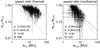 |
Fig. 1 HXR source aspect ratio, wb/wa, as a function of major axis size wa for thermal (left) and nonthermal sources (right). Also shown are power-law fits using the BCES bisector method (dashed lines), the slope α and intercept b of the obtained power law, the rank correlation coefficient R, and the number of value pairs, N. The dotted lines represent the lower threshold on wb/wa imposed by RHESSI’s resolution limit of 2′′. Larger sources have smaller aspect ratios, i.e., are more elongated. |
In addition to the slope and intercept, α and b (including standard deviation), the plots show Spearman’s rank correlation coefficient R and the number of value pairs N (includes all fitted sources from each event). For both types of sources, there is a clear tendency (R ≤ −0.65) for larger sources to have smaller aspect ratios, which means that larger sources tend to be more elongated. Assuming that the thermal emission comes from loops (or bundles of loops), this implies that with growing geometric sizes, the loop length increases at a higher rate than the loop width. This agrees with the characteristics of loops in active regions transient brightenings observed by Yohkoh/SXT (Shimizu 1995).
The decrease in the aspect ratio is even more pronounced in the case of the footpoints: there is a well-defined (R = −0.8), inversely linear (α ≈ −1) relationship with major axis size. This means that while wa,nth increases strongly for larger sources, wb,nth only grows modestly. In other words, the areas Anth,FP of the footpoints are mainly determined by their major axis. It is expected that the major axes are aligned with the flare ribbons (Liu et al. 2007; Dennis & Pernak 2009). Thus it is primarily the length of the nonthermal HXR source along the flare ribbon that determines the footpoint area. This is consistent with the notion proposed by Dennis & Pernak (2009) that the footpoints are actually ribbons with thicknesses that are comparable to the flare ribbons seen in EUV.
There is a lower threshold on the derived source dimensions and aspect ratios imposed by RHESSI’s resolution limit of 2′′. For the thermal sources, wa and wb/wa are well above these limits. While this is also true for the nonthermal sources, the corresponding aspect ratios are closer to the limit and show a similar slope. This could imply that the minor axes are not well resolved, a notion suggested by Dennis & Pernak (2009) and supported in our Paper I.
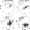 |
Fig. 2 As in Fig. 1, but showing major and minor axes, wa (left) and wb (right), as a function of footpoint separation, dFP, for thermal (top) and nonthermal sources (bottom). |
Next, we study the dependence of the different geometric parameters on the length scale L. As an example, a purely Euclidian scaling would result in source linear dimensions, areas, and volumes being proportional to L to the first, second, and third powers, respectively. In contrast, the volume of filamentary structures, such as thin loops, scales linearly with L. In the following, we adopt the footpoint separation dFP as length scale. This quantity has the advantage of being very well measured by RHESSI (relative uncertainties on the order of 3%), and that it is directly proportional to the loop length l (l = dFPπ/2), which is often used as length scale in studies of scaling relationships. For instance, this is the case in the well-known RTV law (Rosner et al. 1978), which is a theoretical scaling law between pressure, peak temperature, and loop length in static coronal loops.
The two upper plots in Fig. 2 depict the relationship of the major and minor axes of the thermal sources with dFP, while the lower row shows the same relationship for the nonthermal footpoints (only cotemporal measurements are included). In the thermal case, both wa,th and wb,th are moderately well correlated with dFP, the correlation being more pronounced for wb,th. The major axis wa,th is linearly related to dFP (α = 1), whereas wb,th rises slightly less steeply with increasing dFP (α = 0.76). This reflects that larger thermal sources have a smaller aspect ratio. In contrast to the thermal sources, the footpoint sizes show a very weak dependence on dFP (R ≈ 0.2).
We now progress to the relationship of the source areas to dFP, which is shown in Fig. 3. As was to be expected from the behavior of the linear sizes, the thermal source areas Ath are fairly well correlated with dFP (R = 0.56), with a power-law slope of α = 1.62 ± 0.11, which is a scaling that is slightly lower than Euclidian (α = 2), but not too far from it. Remarkably, the power-law index is consistent with the ones found by Aschwanden & Parnell (2002) for EUV microflares and by Aschwanden & Aschwanden (2008a) for the scaling of maximum fractal flare area with length scale derived from TRACE EUV data. In the latter study, the length scale was defined as the square root of the total flare area. For the footpoints, the correlation of total area Anth,tot with dFP is somewhat better than for the linear sizes, but still quite modest (R = 0.32). In contrast to the thermal source area, the footpoint area only increases roughly linearly with length scale.
Finally, Fig. 4 shows the relationship of the direct and indirect thermal source volumes with footpoint separation. Since it is derived directly from the thermal source area, Vdir shows the same reasonable correlation with dFP as Ath (R = 0.55), and correspondingly the scaling (α = 2.37 ± 0.17) is slightly below a Euclidian one (α = 3). We point out that Vdir at the time of the SXR maximum, which is most relevant for determining the maximum thermal energy of the hot plasma, actually shows an even stronger correlation (R = 0.9) with the footpoint separation. On the other hand, Vind is well correlated with dFP (R = 0.77), which is to be expected since dFP explicitly enters into the calculation of Vind. With α = 1.54, the scaling of Vind with dFP is not as steep as for the direct thermal volume, and it results from Anth,tot being only weakly correlated with dFP.
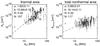 |
Fig. 3 As in Fig. 1, but showing thermal and total nonthermal source areas, Ath (left) and Anth,tot (right), as a function of footpoint separation, dFP. |
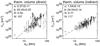 |
Fig. 4 As in Fig. 1, but showing direct and indirect thermal source volumes, Vdir (left) and Vind (right), as a function of footpoint separation, dFP. |
Summarizing, we have found that the scaling of the direct thermal volume Vdir with footpoint separation is slightly below a 3D Euclidian scaling, albeit with significant scatter, while the indirectly determined volume Vind rises significantly less steeply with length scale. This explains why we found in Paper I (Sect. 3.3) that the scatter plot of Vind versus Vdir can be fit with a power law with a slope of less than unity (α = 0.63). This different behavior again poses the question of the validity of the two methods for volume estimation. While Vdir is calculated from quantities that can be measured reasonably well (i.e., at the 10% level) – wa,th and wb,th – Vind depends on dFP, which can be determined with a very high accuracy, but also on the footpoint sizes, which have significantly higher uncertainties (as shown in Paper I). Moreover, the footpoints sizes can be measured during a much shorter time interval than the thermal source (see Paper I, Sect. 3.3). Finally, the indirect method adopts an oversimplified flare model, because all it assumes that all thermal emission is coming from a semicircular loop whose cross-section is determined by the nonthermal footpoint areas. While the footpoints encompass the bases of magnetic loops onto which the bulk of the energy is released in the form of nonthermal electrons at any given time – and which are thus the locations of most plasma evaporation and heating – thermal plasma can also be present in other magnetic structures: in loops where electron acceleration is no longer taking place, but which still emit thermal HXRs until the plasma has cooled down due to radiative and conductive losses, and possibly also in loops that are associated with nonthermal electron fluxes that are too low to generate observable footpoints.
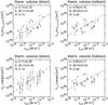 |
Fig. 5 Thermal coronal source volumes derived with the direct (Vdir; left column) and indirect method (Vind; right column) as a function of peak GOES soft X-ray flux ISXR (i.e., GOES class; ISXR = 10-6 W m-2 is a C1 flare, while ISXR = 10-4 W m-2 represents an X1 flare) for the 24 flares analyzed. The upper row shows the volumes at the time of the GOES X-ray peak (t = tmax,SXR), while the lower row depicts the mean values of the volumes, with the error bars showing the whole range from minimum to maximum. Also shown are power-law fits using the BCES bisector method (dashed lines), the slope α and intercept b of the obtained power law, and the rank correlation coefficient, R. |
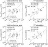 |
Fig. 6 As in Fig. 5, but showing the total nonthermal footpoint areas Anth,tot (left column) and the footpoint separation dFP (right column) as a function of peak GOES soft X-ray flux ISXR. The upper row shows Anth,tot and dFP at the time of the GOES SXR peak, while the lower row depicts the mean values of the volumes, with the error bars showing the whole range from minimum to maximum. For Anth,tot, we additionally show power-law fits obtained with the WLS method (gray dotted line). |
We thus conclude that the direct method gives a more reliable estimate of the volume of the hot plasma in solar flares and that the scaling of this volume with length is close to Euclidian. This is generally consistent with studies of scaling relationships using EUV data, which found fractal scalings of volume with area with exponents of α ≈ 4/3 (Aschwanden & Parnell 2002) and α ≈ 5/3 (Aschwanden 2004), which is also not too far from the Euclidian case (V(A) ~ A3/2).
4. Scaling of geometric parameters with flare importance
After having studied the relationship between the different geometric parameters themselves, we move to the question if the source sizes are related with flare importance as parameterized by the GOES class. The GOES importance is given by the peak SXR flux during a flare. The SXR flux is dependent on temperature, electron density, and volume of the thermal plasma. It would thus be expected that flares with larger plasma volumes are associated with higher GOES peak fluxes. This is predicted by the RTV scaling law (Rosner et al. 1978), and has actually been found by studies using SXR and EUV data (e.g. Shimizu 1995; Ofman et al. 1996; Aschwanden & Parnell 2002; Aschwanden & Aschwanden 2008b). In contrast to this, a study of RHESSI microflares did not reveal any correlation between thermal HXR source volume and GOES class (Hannah et al. 2008), and in Paper I (Sect. 3.3) we found a distribution function of volumes that was consistent with the microflares of Hannah et al. (2008), which suggests that volume is not a crucial factor for flare importance.
To investigate this discrepancy in more detail, we plot the thermal volumes of our events versus the peak GOES SXR flux ISXR (i.e., GOES class; ISXR = 10-6 W m-2 is a C1 flare, while ISXR = 10-4 W m-2 represents an X1 flare) in Fig. 5. The upper row of the figure shows Vdir and Vind at the time of the GOES X-ray peak, which is probably close to the time of maximum thermal energy (e.g. Saint-Hilaire & Benz 2002). The volume Vdir is well correlated with GOES class (R = 0.74), while Vind shows a weaker correlation (R = 0.46). The direct volume Vdir increases slightly more strongly with importance than Vind (α = 0.74 ± 0.1 vs. α = 0.59 ± 0.1). The lower row of Fig. 5 depicts the mean values of Vdir and Vind, with the error bars showing the whole range from minimum to maximum in each event. The mean values of both Vdir and Vind correlate as well with the GOES class as the values at peak SXR flux, and they also show a similar scaling.
Figure 6 shows the correlation of GOES magnitude with the geometric parameters Anth,tot and dFP of the nonthermal footpoints. Just as for the relation with length scales, the footpoint areas do not show any significant correlation with GOES class (R ≤ 0.17). This is the case for the areas at the time of the SXR peak (in those cases where footpoints could not be measured at that time, the areas that were closest in time were used instead), as well as for the mean values of Anth,tot. In contrast to the other correlations, the power laws obtained with the BCES bisector method evidently provide a very poor fit in this case, as seen by the large uncertainties of the fit parameters. We therefore also show a weighted linear least-squares (WLS) fit – log y on log x – which apparently works better in this case.
The lack of correlation of the footpoint areas with length scale could partly be due to resolution problems. In Paper I, we concluded that RHESSI imaging approaches its limits when it comes to measuring the sizes of small footpoints, in particular their minor axis. When weak flares are indeed associated with smaller footpoints, we would derive artificially large footpoint areas due to the resolution limit, and the correlation could be obscured. Potentially, albedo could also play a role here, since it will increase the measured sizes of the sources imaged in the range of 25−50 keV more strongly than those of sources imaged at higher energies. Since all C class flares were imaged at 25−50 keV, their footpoints could appear larger than they are as compared to the stronger flares. However, the albedo component has a much lower flux density than the footpoints and is therefore unlikely to influence the FWHM measurements significantly (see also Battaglia et al. 2011).
In contrast, the footpoint separations show a reasonable correlation with flare importance (R = 0.59), with a power-law index of α = 0.39 ± 0.08. This generally agrees with the relationship between length scale and flare magnitude obtained for the 20 flares considered by Aschwanden & Aschwanden (2008a), for which α = 0.3 ± 0.08 and R = 0.79 were found, even though the length scale was derived in this study in a totally different manner, namely from the flare area observed in EUV.
Based on these results we can conclude that flares in the range of class C to the largest X flares do show a correlation of thermal volume – and footpoint separation – with flare magnitude. However, why is this not the case for the microflares studied by Hannah et al. (2008)? One possibility could be that while the energy required for microflares can be provided by magnetic field structures of almost any spatial size, the larger amount of energy required for stronger flares tends to be more strongly associated with larger magnetic structures. This could explain the apparent discrepancy in scaling between geometric flare size and magnitude.
5. Temporal evolution of source sizes
We have noted in the introduction that the significant temporal evolution of the HXR spectrum is probably not consistent with constant sources sizes. The ranges of the different geometric parameters for each event given in Table 1 and shown as error bars in Figs. 5 and 6 have proven that there is indeed significant variation. We thus have to consider the temporal evolution of source sizes in more detail. We focus on the two geometric parameters that are essential for calculating important physical quantities: the thermal volume (which determines thermal energy and electron density) and the nonthermal footpoint area (required for the nonthermal energy flux density). Moreover, we consider the footpoint separation as a characteristic length scale.
5.1. Thermal coronal sources
Which temporal evolution would we expect for the volume of the thermal plasma? The thermal source will appear when the energy release reaches a level where significant amounts of plasma are either heated directly in the corona or evaporated from the chromosphere. As more and more magnetic field lines with increasing spatial scales become reconnected, an increasing number of loops is filled with hot and dense plasma, so we would expect the thermal volume to grow. When the energy release drops off around the time of peak SXR and thermal HXR flux, and the loops cool down because of radiative and conductive losses, we expect to see a decrease in thermal source volume, since more and more plasma drops below RHESSI’s temperature range. This growth-decline behavior is common for flares observed in the EUV (e.g. Aschwanden & Aschwanden 2008b). Is this also true in the thermal HXR range?
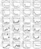 |
Fig. 7 Temporal evolution of the thermal source volume Vdir for all 24 flares. For comparison, the upper parts of the individual plots show the HXR lightcurves in the 6−12 keV (thermal; black line) and the 50−100 keV channels (nonthermal; gray line), respectively, in units of counts per second and detector. The dashed lines denote the time of the GOES SXR peak flux in the 1−8 Å band. |
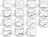 |
Fig. 8 Temporal evolution of the thermal coronal source height hcor compared to the thermal source volume Vdir for 15 selected flares. In most events the source heights are correlated with the thermal volumes. |
Figure 7 shows the temporal evolution of the thermal source volume Vdir for all 24 flares4. As context, the upper parts of the individual plots show the HXR count rate (corrected count rate; in counts per second and detector) in the thermal 6−12 keV and the nonthermal 50−100 keV range (a range of 25−50 keV was selected for events 1, 3, 4, 5, and 8). Inspecting Fig. 7, we first find that time of the GOES peak flux – a proxy for maximum thermal energy – is associated with a maximum of the thermal volume only in a few events. There is a clear association with the maximum volume in event 19, and a less clear association with local maxima of Vdir in an additional five events (4, 9, 12, 13, and 24). This implies that the maximum SXR emission, hence maximum thermal energy, is not predominantly determined by the thermal plasma volume5. Therefore, plasma density and/or temperature have to be a more important factor.
We now focus on the early phase of the events, i.e. times well before the SXR peak (roughly, this corresponds to the impulsive phase). In the simple picture described above, we would expect the volume to increase steadily in this phase. However, we find that this is actually the case in only three events (19, 21, and 22; all X-class flares). In all other cases (omitting event 24, for which we do not have RHESSI observations of the early phase), the volume shows a pronounced early peak: in eleven events (1, 3, 5, 8, 9, 11, 12, 13, 14, 16, 18), we have detected a rapid rise to a peak and then a decrease, and in an additional nine cases (2, 4, 6, 7, 10, 15, 17, 20, 23), measurements already start at the peak values. In the latter cases, the rapid inital rise of Vdir could probably not be detected due to insufficient counts. On average, the maximum volumes of the early peaks are three times as large as the volumes at the times of maximum SXR flux, and they occur primarily at the very beginning of the impulsive phase. In the majority of 16 events, the early volumes are actually the maximum values that are not reached again over the course of the flares’ evolution.
Are these surprisingly large initial volumes real, or could they be some artifact? The possibility that the early peaks are imaging algorithm artifacts is minimized by our approach of using four different algorithms (see Paper I). While the uncertainties of the volumes (the error bars in Fig. 7 representing the standard deviation of the volumes as given by the different methods) tend to be larger than during the “main phase” of the flares, the peaks are still significant. Different attenuator states also cannot provide an explanation: large early volumes were found with all attenuator states (A0, A1, and A3), and regardless of whether the attenuator state changed during the event. A third possibility for an artifact are count statistics: since count rates are low in the early phase of the flares (see thermal HXR lightcurves in Fig. 7), it could be possible that early thermal images have too few counts to image the thermal sources properly. However, after plotting counts per image versus derived volume for all imaged thermal sources, we could not find any significant trend towards low counts being associated with significantly larger volumes. Typically, image counts associated with the large initial volumes could also be found for significantly smaller volumes.
 |
Fig. 9 As in Fig. 7, but showing the temporal evolution of the total footpoint areas Anth,tot and the footpoint separations dFP for all 24 flares. |
Having made these checks, we conclude that large thermal sources are indeed common in the early impulsive phase of solar flares. This finding is somewhat surprising and contrasts with flare observations in other wavelength bands such as EUV (e.g. Aschwanden & Aschwanden 2008b), but it is consistent with what had been reported for the 2003 Jul. 23 flare (Lin et al. 2003).
How can we physically make sense of these large initial volumes? They could result from the contraction of magnetic loops in the early flare phase that was deduced from the initial downward motion of thermal coronal sources. This behavior was first observed by Sui & Holman (2003) for event 8 in our study, and has since been confirmed for several other flares (e.g. Sui et al. 2004; Liu et al. 2004; Veronig et al. 2006; Joshi et al. 2007). To check this possibility, we compared the evolution of the thermal source volumes with their heights. The heights hcor of the coronal sources were computed by taking the plane-of-sky distance of the thermal source centroid from the midpoint between the two footpoints on the solar surface and dividing it by the sine of the heliocentric angle. While this gives quantitatively accurate values for hcor only for sources centered between the footpoints that are moving radially, for our purposes the relative heights during the flares’ evolution are sufficient. To minimize the influence of projection effects, we have excluded events with a heliocentric angle of less than 25°, events for which unrealistically small heights (i.e. less than 0.2 times the footpoint separation and less than 0.5 times the minor thermal source axis) were obtained, and events with complex source morphology. This has left 15 flares, for which the temporal evolution of source height hcor in comparison with the thermal volume Vdir is shown in Fig. 8.
Inspection of hcor in Fig. 8 shows that an initial downward motion of the coronal source is actually a common behavior in flares, because it is evident in 12 out of 15 events (it is absent only in events 16, 17, and 19)6. A comparison with Vdir shows that the downward motion is indeed correlated with the large inital volumes in the majority of events. Similarly, in the later phase the rise of the coronal sources – evident in all events – is associated with the increase in the volume. For some events (e.g. second row from top in Fig. 8), the evolution of hcor and Vdir is strikingly similar.
In the nine events with both an early peak in volume and an initial downward motion of the coronal source, the maximum source height in the early phase is on the average about twice as large as the minimum source height that is reached before the gradual rise of the source begins in the later phase. Assuming a scaling of  with a power-law index of α = 2.37, as was derived for the scaling of volume with length scale in Sect. 3, this would lead to early volumes being 5.4 times larger than the volumes at the times of minimum source height. With a value of 4.9, the actual measured ratio is very close to that. We conclude that at least in the events where a downward moving thermal source corresponds with a decreasing volume, the contraction of magnetic loops can actually explain the early peaks in the temporal evolution of the thermal source volume.
An additional influence on the early evolution of the thermal volume could come from the fact that initially plasma heated directly in the corona (e.g. at the slow-mode shocks; cf. Petschek 1964; Cargill & Priest 1982) will be observed, while with increasing nonthermal energy input, the plasma resulting from chromospheric evaporation will begin to dominate the emission. Since the locally heated plasma will be significantly less dense than the evaporated one, RHESSI will not be able to observe the more tenuous source owing to dynamic range limitations. It thus could be that a large tenuous source, possibly corresponding to the cusp that is sometimes observed in the EUV and SXR in the later phase (e.g. Tsuneta et al. 1992; Hara et al. 2008), is still present after the early phase. We will investigate this possibility with the help of HXR spectral data in a forthcoming paper.
We now shift our attention to the later phase of the events. Fourteen flares show an increasing volume in the late phase: in eight events (10, 13, 15, 18, 19, 21, 22, 23), the volume increases to a maximum and then begins to decrease, while in a further seven events (2, 5, 12, 14, 17, 18, 20) the final decrease is absent, either due to the end of the observing time interval, or possibly due to insufficient counts. In the remaining flares, the volumes stay approximately constant. The rising and the decreasing volumes are consistent with the simple scenario described at the beginning of this section (a succession of loops or an arcade that is growing as magnetic reconnection progresses), but it is not synchronized with the SXR (or thermal HXR) lightcurve. For example, compare events 21 and 22 (lower left in Fig. 7). While the SXR peak occurs during the volume increase in event 21, it is located well within the phase of decreasing volume in event 22. Again, this indicates that volume is not the dominant factor in determining the thermal emission, and that electron density and/or temperature are more important. We will study this issue in a forthcoming paper where we will be combining geometric with spectral parameters. In principle the presence of an extended source can be inferred from the relative intensities of the modulation amplitudes given by the finer and coarser subcollimators (Schmahl & Hurford 2002).
5.2. Nonthermal footpoint sources
Having studied the temporal evolution of the thermal source volumes, we now consider the total areas of the nonthermal footpoints and their separation. Figure 9 shows the evolution of both Anth,tot and dFP for all 24 flares. It is immediately evident that the nonthermal sources can be measured during significantly shorter time intervals than the thermal sources. Typically, Anth,tot could be reliably measured in only a few time intervals per event. Only in five X-class flares could Anth,tot and dFP be tracked over more than ten minutes. The total footpoint area does not show any significant trends in its temporal evolution: most of its fluctuations are erratic and predominantly not statistically significant (see the error bars on Anth,tot). There is also no correlation with the nonthermal HXR count rate. We conclude that any evolution that might be there is below the limits given by our relatively large uncertainties.
In contrast to Anth,tot, dFP does show a clear trend in temporal evolution, at least for the stronger flares with longer impulsive phases: in the events 16, 18, 19, 20, 21, and 23, dFP monotonically increases with time. This is consistent with the footpoints moving away from the polarity inversion line as the reconnected loop system grows, and it has been observed in many solar flares (for a review, see Fletcher et al. 2011).
We have not shown the evolution of Vind derived from Anth,tot and dFP here, since the combination of short time ranges with the relatively large uncertainties of Anth,tot results in a lack of significant trends in the temporal evolution.
6. Conclusions
We have analyzed the scaling relationships and the temporal evolution of the geometric parameters of thermal and nonthermal HXR sources in 24 flares observed by RHESSI, focusing on the volumes of the thermal coronal sources and the areas and separations of the nonthermal footpoints. Starting with the scaling relationships between the different geometric parameters, we found that sources with a larger major axis are associated with a smaller aspect ratio; in other words, larger sources are more elongated. This is true for both thermal and nonthermal sources. In the former case, similar behavior of the aspect ratio was found for the loops in the active region transient brightenings (ARTBs) observed with Yohkoh/SXT (Shimizu 1995), while in the latter case, the behavior of the aspect ratio is consistent with the notion that the footpoints are relatively thin ribbons oriented along the flare ribbons seen in the EUV (cf. Dennis & Pernak 2009). Moreover, there are indications that the minor footpoint axes are not resolved well by RHESSI, which is also reported by Dennis & Pernak (2009) and supported by our findings in Paper I.
Adopting the separation of the footpoints, dFP, as a characteristic length, we studied the dependence of different geometric parameters on this length scale. We found that the volume of the thermal plasma that is derived directly from the thermal source size, Vdir, shows a scaling with dFP that is not too far from the Euclidian case (i.e.,  ), albeit with significant scatter. Given this scatter, our result generally agrees with the fractal scalings of volume with area derived from high-resolution EUV data (Aschwanden & Parnell 2002; Aschwanden 2004), which are also not too far from Euclidian. Note here that we could only consider the apparent volumes, whereas the true plasma-filled volumes can be smaller due to filling factors of less than unity (see e.g. Aschwanden & Aschwanden 2008b).
We found that both the thermal source volumes and the nonthermal footpoint separations are fairly well correlated with flare importance as parameterized by the GOES peak SXR intensity: more intense flares have larger thermal volumes and larger footpoint separations. This agrees with the results of several earlier studies of flares, microflares, and nanoflares using EUV and SXR data (Shimizu 1995; Ofman et al. 1996; Aschwanden & Parnell 2002; Aschwanden & Aschwanden 2008b), and is also predicted by theory, e.g. by the RTV scaling law (Rosner et al. 1978). It is therefore quite surprising that Hannah et al. (2008) did not find any correlation between volume and flare importance for their large sample of RHESSI microflares. One possible explanation for this discrepancy would be that the comparatively small amount of energy required for microflares can be provided by magnetic structures of almost any size, while the higher energies required to power stronger flares tend to be associated more with field structures of a larger spatial size. However, this issue will require more detailed investigation. In contrast to thermal volumes and footpoint separations, the footpoint areas do not show any significant correlation with GOES class.
We found a significant temporal evolution of the source volumes for most events. This implies that just using a fixed source volume (usually taken at the time of the SXR or thermal HXR peak) for the study of a whole event may be misleading. Generally, the temporal evolution of the volume is not well correlated with the SXR or thermal HXR lightcurves, which implies that electron density and/or temperature are more important factors in determining thermal emission and energy.
The thermal source volume as derived from EUV and SXR observations (e.g., Aschwanden & Aschwanden 2008b; Tsuneta et al. 1992; Berghmans et al. 2001) initially shows a growing volume (as more field lines become reconnected and subsequently filled with hot and dense plasma), which is followed by a decrease in the observed volume (as the plasma cools and drops out of the observable temperature range7). Many RHESSI sources behave in a more complex manner. In particular, the majority of events showed a steep initial growth of the volume to an early peak. These large initial volumes often occur at the same time as the initial downward motion of coronal sources that has been reported before (e.g. Sui & Holman 2003). We found for the first time that the initial downward motion is actually rather common (present in 87% of events), as are the large early volumes (also in 87% of cases). We concluded that the behavior of coronal source height and volume in the early phase is consistent with the initial contraction of reconnected magnetic loops. After this early phase, most flares showed a gradually growing volume, which in about half of the events was followed by a slow decrease. This is consistent with what is observed in EUV and SXR. On a more general level, we have reached the same conclusion as in Paper I that the source volumes derived directly from the thermal coronal sources (Vdir) should be preferred to those obtained indirectly from the footpoint areas and separations (Vind).
We could not detect significant trends in the temporal evolution of the area of the nonthermal footpoints. This could be partly due to the relatively large uncertainties of the nonthermal area, which are possibly caused by resolution issues. In contrast, we clearly observed a growing separation of the footpoints in all flares, consistent with the growth of the reconnected loop system.
In summary, most of our findings on the behavior of the geometric parameters of thermal and nonthermal HXR sources are consistent with the standard model of eruptive solar flares (cf. the CSHKP model; Carmichael 1964; Sturrock 1966; Hirayama 1974; Kopp & Pneuman 1976). While the surprising finding of large thermal source volume in the early phase of most flares is consistent with initially contracting field lines, different plasma ensembles – locally heated coronal versus evaporated chromospheric material – could also play a role.
In a forthcoming paper, we will combine the geometric parameters of the HXR sources with the physical parameters derived from HXR spectroscopy. This will allow time-resolved study of quantities such as thermal energy, conductive and radiative energy loss, and nonthermal energy flux density, which are crucial for understanding energy release and particle acceleration in solar flares.
For a review, see Fletcher et al. (2011).
Not deselecting methods for individual events has a negligible influence on the results of both paper I and this paper.
For the thermal sources, we have deconvolved for the CLEAN beam (e.g. Saint-Hilaire & Benz 2002), while for the nonthermal sources we used the CLEAN component method of Dennis & Pernak (2009).
Here, we do not consider the evolution of Vind, since it could be obtained only over limited time ranges.
The same result is obtained when using thermal HXRs in the range of 6–12 keV from RHESSI instead of SXRs from GOES.
In event 19, an early downward motion was actually detected by Liu et al. (2004) and Veronig et al. (2006). It is missing here because the source sizes could not be determined accurately in the early phase.
Compared to EUV, SXR loops remain bright for longer time intervals thanks to the broader temperature response of SXR instruments.
Acknowledgments
The work of A. W. was supported by DLR under grant No. 50 QL 0001. The authors are grateful to the RHESSI Team (PI: R. P. Lin) for free access to the data and the development of the software.
References
- Akritas, M. G., & Bershady, M. A. 1996, ApJ, 470, 706 [NASA ADS] [CrossRef] [Google Scholar]
- Aschwanden, M. J. 2004, Physics of the Solar Corona. An Introduction (Springer) [Google Scholar]
- Aschwanden, M. J., & Aschwanden, P. D. 2008a, ApJ, 674, 530 [NASA ADS] [CrossRef] [Google Scholar]
- Aschwanden, M. J., & Aschwanden, P. D. 2008b, ApJ, 674, 544 [NASA ADS] [CrossRef] [Google Scholar]
- Aschwanden, M. J., & Parnell, C. E. 2002, ApJ, 572, 1048 [NASA ADS] [CrossRef] [Google Scholar]
- Aschwanden, M. J., Brown, J. C., & Kontar, E. P. 2002, Sol. Phys., 210, 383 [NASA ADS] [CrossRef] [Google Scholar]
- Battaglia, M., Kontar, E. P., & Hannah, I. G. 2011, A&A, 526, A3 [NASA ADS] [CrossRef] [EDP Sciences] [Google Scholar]
- Berghmans, D., McKenzie, D., & Clette, F. 2001, A&A, 369, 291 [NASA ADS] [CrossRef] [EDP Sciences] [Google Scholar]
- Cargill, P. J., & Priest, E. R. 1982, Sol. Phys., 76, 357 [NASA ADS] [CrossRef] [Google Scholar]
- Carmichael, H. 1964, NASA SP, 50, 451 [Google Scholar]
- Dennis, B. R., & Pernak, R. L. 2009, ApJ, 698, 2131 [NASA ADS] [CrossRef] [Google Scholar]
- Emslie, A. G., Kucharek, H., Dennis, B. R., et al. 2004, J. Geophys. Res., 109, 10104 [NASA ADS] [CrossRef] [Google Scholar]
- Fletcher, L., Dennis, B. R., Hudson, H. S., et al. 2011, Space Sci. Rev., 159, 19 [NASA ADS] [CrossRef] [Google Scholar]
- Grigis, P. C., & Benz, A. O. 2004, A&A, 426, 1093 [NASA ADS] [CrossRef] [EDP Sciences] [Google Scholar]
- Hannah, I. G., Christe, S., Krucker, S., et al. 2008, ApJ, 677, 704 [NASA ADS] [CrossRef] [Google Scholar]
- Hara, H., Watanabe, T., Matsuzaki, K., et al. 2008, PASJ, 60, 275 [NASA ADS] [Google Scholar]
- Hirayama, T. 1974, Sol. Phys., 34, 323 [NASA ADS] [CrossRef] [Google Scholar]
- Holman, G. D., Sui, L., Schwartz, R. A., & Emslie, A. G. 2003, ApJ, 595, L97 [NASA ADS] [CrossRef] [Google Scholar]
- Hurford, G. J., Schmahl, E. J., Schwartz, R. A., et al. 2002, Sol. Phys., 210, 61 [NASA ADS] [CrossRef] [Google Scholar]
- Hurford, G. J., Schmahl, E. J., & Schwartz, R. A. 2005, AGU Abstr. Spring, A12 [Google Scholar]
- Isobe, T., Feigelson, E. D., Akritas, M. G., & Babu, G. J. 1990, ApJ, 364, 104 [NASA ADS] [CrossRef] [EDP Sciences] [Google Scholar]
- Joshi, B., Manoharan, P. K., Veronig, A. M., Pant, P., & Pandey, K. 2007, Sol. Phys., 242, 143 [NASA ADS] [CrossRef] [Google Scholar]
- Kontar, E. P., Hannah, I. G., & MacKinnon, A. L. 2008, A&A, 489, L57 [NASA ADS] [CrossRef] [EDP Sciences] [Google Scholar]
- Kopp, R. A., & Pneuman, G. W. 1976, Sol. Phys., 50, 85 [NASA ADS] [CrossRef] [Google Scholar]
- Krucker, S., Fivian, M. D., & Lin, R. P. 2005, Adv. Space Res., 35, 1707 [NASA ADS] [CrossRef] [Google Scholar]
- Lin, R. P., Dennis, B. R., Hurford, G. J., et al. 2002, Sol. Phys., 210, 3 [Google Scholar]
- Lin, R. P., Krucker, S., Hurford, G. J., et al. 2003, ApJ, 595, L69 [NASA ADS] [CrossRef] [Google Scholar]
- Liu, C., Lee, J., Gary, D. E., & Wang, H. 2007, ApJ, 658, L127 [NASA ADS] [CrossRef] [Google Scholar]
- Liu, W., Jiang, Y. W., Liu, S., & Petrosian, V. 2004, ApJ, 611, L53 [NASA ADS] [CrossRef] [Google Scholar]
- Liu, W., Petrosian, V., Dennis, B. R., & Holman, G. D. 2009, ApJ, 693, 847 [NASA ADS] [CrossRef] [Google Scholar]
- Mann, G., & Warmuth, A. 2011, A&A, 528, A104 [NASA ADS] [CrossRef] [EDP Sciences] [Google Scholar]
- Mann, G., Warmuth, A., & Aurass, H. 2009, A&A, 494, 669 [NASA ADS] [CrossRef] [EDP Sciences] [Google Scholar]
- Metcalf, T. R., Hudson, H. S., Kosugi, T., Puetter, R. C., & Pina, R. K. 1996, ApJ, 466, 585 [NASA ADS] [CrossRef] [Google Scholar]
- Miklenic, C. H., Veronig, A. M., Vršnak, B., & Hanslmeier, A. 2007, A&A, 461, 697 [Google Scholar]
- Ofman, L., Davila, J. M., & Shimizu, T. 1996, ApJ, 459, L39 [NASA ADS] [CrossRef] [Google Scholar]
- Petschek, H. E. 1964, NASA SP, 50, 425 [Google Scholar]
- Rosner, R., Tucker, W. H., & Vaiana, G. S. 1978, ApJ, 220, 643 [NASA ADS] [CrossRef] [Google Scholar]
- Saint-Hilaire, P., & Benz, A. O. 2002, Sol. Phys., 210, 287 [NASA ADS] [CrossRef] [Google Scholar]
- Saint-Hilaire, P., & Benz, A. O. 2005, A&A, 435, 743 [NASA ADS] [CrossRef] [EDP Sciences] [Google Scholar]
- Schmahl, E. J., & Hurford, G. J. 2002, Sol. Phys., 210, 273 [NASA ADS] [CrossRef] [Google Scholar]
- Schmahl, E. J., Pernak, R. L., Hurford, G. J., Lee, J., & Bong, S. 2007, Sol. Phys., 240, 241 [NASA ADS] [CrossRef] [Google Scholar]
- Shimizu, T. 1995, Pub. Astron. Soc. Jap., 47, 251 [Google Scholar]
- Sturrock, P. A. 1966, Nature, 211, 695 [NASA ADS] [CrossRef] [Google Scholar]
- Sui, L., & Holman, G. D. 2003, ApJ, 596, L251 [NASA ADS] [CrossRef] [Google Scholar]
- Sui, L., Holman, G. D., & Dennis, B. R. 2004, ApJ, 612, 546 [NASA ADS] [CrossRef] [Google Scholar]
- Tsuneta, S., Hara, H., Shimizu, T., et al. 1992, Publ. Astron. Soc. Jpn., 44, L63 [Google Scholar]
- Veronig, A. M., Brown, J. C., Dennis, B. R., et al. 2005, ApJ, 621, 482 [Google Scholar]
- Veronig, A. M., Karlický, M., Vršnak, B., et al. 2006, A&A, 446, 675 [Google Scholar]
- Warmuth, A., & Mann, G. 2013, A&A, 552, A86 [NASA ADS] [CrossRef] [EDP Sciences] [Google Scholar]
- Warmuth, A., Holman, G. D., Dennis, B. R., et al. 2009a, ApJ, 699, 917 [NASA ADS] [CrossRef] [Google Scholar]
- Warmuth, A., Mann, G., & Aurass, H. 2009b, A&A, 494, 677 [NASA ADS] [CrossRef] [EDP Sciences] [Google Scholar]
All Tables
All Figures
|
Fig. 1 HXR source aspect ratio, wb/wa, as a function of major axis size wa for thermal (left) and nonthermal sources (right). Also shown are power-law fits using the BCES bisector method (dashed lines), the slope α and intercept b of the obtained power law, the rank correlation coefficient R, and the number of value pairs, N. The dotted lines represent the lower threshold on wb/wa imposed by RHESSI’s resolution limit of 2′′. Larger sources have smaller aspect ratios, i.e., are more elongated. |
| In the text | |
|
Fig. 2 As in Fig. 1, but showing major and minor axes, wa (left) and wb (right), as a function of footpoint separation, dFP, for thermal (top) and nonthermal sources (bottom). |
| In the text | |
|
Fig. 3 As in Fig. 1, but showing thermal and total nonthermal source areas, Ath (left) and Anth,tot (right), as a function of footpoint separation, dFP. |
| In the text | |
|
Fig. 4 As in Fig. 1, but showing direct and indirect thermal source volumes, Vdir (left) and Vind (right), as a function of footpoint separation, dFP. |
| In the text | |
|
Fig. 5 Thermal coronal source volumes derived with the direct (Vdir; left column) and indirect method (Vind; right column) as a function of peak GOES soft X-ray flux ISXR (i.e., GOES class; ISXR = 10-6 W m-2 is a C1 flare, while ISXR = 10-4 W m-2 represents an X1 flare) for the 24 flares analyzed. The upper row shows the volumes at the time of the GOES X-ray peak (t = tmax,SXR), while the lower row depicts the mean values of the volumes, with the error bars showing the whole range from minimum to maximum. Also shown are power-law fits using the BCES bisector method (dashed lines), the slope α and intercept b of the obtained power law, and the rank correlation coefficient, R. |
| In the text | |
|
Fig. 6 As in Fig. 5, but showing the total nonthermal footpoint areas Anth,tot (left column) and the footpoint separation dFP (right column) as a function of peak GOES soft X-ray flux ISXR. The upper row shows Anth,tot and dFP at the time of the GOES SXR peak, while the lower row depicts the mean values of the volumes, with the error bars showing the whole range from minimum to maximum. For Anth,tot, we additionally show power-law fits obtained with the WLS method (gray dotted line). |
| In the text | |
|
Fig. 7 Temporal evolution of the thermal source volume Vdir for all 24 flares. For comparison, the upper parts of the individual plots show the HXR lightcurves in the 6−12 keV (thermal; black line) and the 50−100 keV channels (nonthermal; gray line), respectively, in units of counts per second and detector. The dashed lines denote the time of the GOES SXR peak flux in the 1−8 Å band. |
| In the text | |
|
Fig. 8 Temporal evolution of the thermal coronal source height hcor compared to the thermal source volume Vdir for 15 selected flares. In most events the source heights are correlated with the thermal volumes. |
| In the text | |
|
Fig. 9 As in Fig. 7, but showing the temporal evolution of the total footpoint areas Anth,tot and the footpoint separations dFP for all 24 flares. |
| In the text | |
Current usage metrics show cumulative count of Article Views (full-text article views including HTML views, PDF and ePub downloads, according to the available data) and Abstracts Views on Vision4Press platform.
Data correspond to usage on the plateform after 2015. The current usage metrics is available 48-96 hours after online publication and is updated daily on week days.
Initial download of the metrics may take a while.