| Issue |
A&A
Volume 552, April 2013
|
|
|---|---|---|
| Article Number | A80 | |
| Number of page(s) | 18 | |
| Section | Extragalactic astronomy | |
| DOI | https://doi.org/10.1051/0004-6361/201118513 | |
| Published online | 29 March 2013 | |
Dynamical analysis of strong-lensing galaxy groups at intermediate redshift ⋆,⋆⋆,⋆⋆⋆
1 Departamento de Física y Astronomía, Universidad de Valparaíso, Avda. Gran Bretaña 1111, 2360102 Valparaíso, Chile
e-mail: This email address is being protected from spambots. You need JavaScript enabled to view it.
2 Departamento de Astronomía y Astrofísica, Pontificia Universidad Católica de Chile, Avda. Vicuña Mackenna 4860, Casilla 306, Santiago 22, Chile
3 Centro de Investigaciones de Astronomía, AP 264, Mérida 5101–A, Venezuela
4 Aix Marseille Université, CNRS, LAM (Laboratoire d’Astrophysique de Marseille) UMR 7326, 13388 Marseille, France
5 Dark Cosmology Centre, Niels Bohr Institute, University of Copenhagen, Juliane Marie Vej 30, 2100 Copenhagen, Denmark
6 Laboratoire d’Astrophysique de Toulouse-Tarbes, Université de Toulouse, CNRS, 57 avenue d’Azereix, 65000 Tarbes, France
7 Institut d’Astrophysique de Paris, UMR 7095 CNRS & Université Pierre et Marie Curie, 98bis Bd Arago, 75014 Paris, France
8 CRAL, Université Lyon 1, Observatoire de Lyon, 9 avenue Charles André, 69561 Saint Genis Laval Cedex, France
Received: 23 November 2011
Accepted: 7 January 2013
Abstract
We present VLT spectroscopic observations of seven newly discovered galaxy groups between 0.3 < z < 0.7. The groups were selected from the Strong Lensing Legacy Survey (SL2S), a survey that consists of a systematic search for strong lensing systems in the Canada-France-Hawaii Telescope Legacy Survey (CFHTLS). We give details about the target selection, spectroscopic observations, and data reduction for the first release of confirmed SL2S groups. The dynamical analysis of the systems reveals that they are gravitationally bound structures, with at least 4 confirmed members and velocity dispersions between 300 and 800 km s-1. Their virial masses are between 1013 and 1014 M⊙, so they can be classified as groups or low mass clusters. Most of the systems are isolated groups, except two of them that show evidence of an ongoing merger of two substructures. We find that weak lensing estimates of the group velocity dispersions are 50% greater than estimates based upon the radial velocities of its members, and conclude that the dynamics of baryonic matter is a good tracer of the total mass content in galaxy groups.
Key words: galaxies: groups: general / galaxies: kinematics and dynamics / galaxies: evolution / galaxies: high-redshift
Based on observations collected at the European Southern Observatory, Paranal, Chile (Program P80.A-0610B); based on observations obtained with MegaPrime/MegaCam, a joint project of CFHT and CEA/DAPNIA, at the Canada-France-Hawaii Telescope (CFHT), which is operated by the National Research Council (NRC) of Canada, the Institut National des Sciences de l’Univers of the Centre National de la Recherche Scientifique (CNRS) of France, and the University of Hawaii. This work is based in part on data products produced at TERAPIX and the Canadian Astronomy Data Centre as part of the Canada-France-Hawaii Telescope Legacy Survey, a collaborative project of NRC and CNRS.
Appendices are available in electronic form at http://www.aanda.org
Reduced spectra are only available at the CDS via anonymous ftp to cdsarc.u-strasbg.fr (130.79.128.5) or via http://cdsarc.u-strasbg.fr/viz-bin/qcat?J/A+A/552/A80
© ESO, 2013
1. Introduction
Galaxy groups are the most common structures in the Universe, containing at least 50% of all galaxies at the present day (Eke et al. 2004), and they cover the intermediate mass range between large elliptical galaxies and galaxy clusters. A wide array of methods have been used to identify groups at intermediate and high-z: percolation algorithms based on optical photometric and spectroscopic data (Marinoni et al. 2002; Eke et al. 2004; Adami et al. 2005; Yang et al. 2007; Zapata et al. 2009), X-ray emission from hot intragroup gas (Brough et al. 2006; Finoguenov et al. 2009), and bright arcs due to strong lensing (Cabanac et al. 2007; Limousin et al. 2009; More et al. 2012).
The first large sample of groups detected in redshift space was presented by Geller & Huchra (1983), who found 176 groups up to z = 0.03 by using the Center for Astrophysics (CfA) galaxy redshift survey. Nowadays, with the advent of large spectroscopic surveys such as the Two Degree Field Galaxy Redshift Survey (2dFGRS; Colless et al. 2001), the Sloan Digital Sky Survey (SDSS; York et al. 2000), and the Deep Extragalactic Probe 2 Redshift Survey (DEEP2; Davis et al. 2003), well over 5000 groups have been identified up to z ~ 1. Eke et al. (2004) identified about 7000 groups and clusters in the 2dFGRS with at least four members, and found that they cover a wide range in mass between 1012 and 1015 M⊙. At low redshift, Berlind et al. (2006) used a friends-of-friends (FOF) algorithm to identify groups in the SDSS Data Release 2 (DR2; Abazajian et al. 2004) and found about 8100 groups between 0.01 < z < 0.10. At higher redshift, Gerke et al. (2005) found about 900 groups with two or more members between 0.7 < z < 1.4 using the DEEP2 survey.
Recently, Knobel et al. (2012) have presented a sample of about 1500 galaxy groups between redshifts 0.1 and 1.0 that were identified in the zCOSMOS-bright survey (Lilly et al. 2007). They detected clear evidence of the growth of cosmic structure over the past seven billion years because the fraction of galaxies that are found in groups (in volume-limited samples) decreases significantly to higher redshifts.
The analysis of the galaxy content in groups and clusters is essential for understanding the effects of the local environment on galaxy formation and evolution processes. For instance, galaxy collisions are expected to be most effective in less massive groups, where the system velocity dispersions are comparable to the internal velocities of galaxies, leading to strong galaxy-galaxy interactions and therefore enhancing star formation (Mihos & Hernquist 1996). Furthermore, the feedback from supernovae and supermassive black holes on the hot intragroup gas is expected to be relevant in suppressing the onset of catastrophic cooling of the hot gas (e.g. Churazov et al. 2001), since the energy input associated with these sources is comparable to the binding energies of these systems (McCarthy et al. 2010).
The evolution of the stellar and gas content of galaxies strongly depends on the properties of their host galaxy cluster (Oemler 1974). For instance, Hansen et al. (2009) studied a large sample of groups and clusters in the Sloan Digital Sky Survey (SDSS; York et al. 2000), and found that the fraction of red-sequence galaxies increases with cluster mass, and it decreases with cluster-centric distance (see also Padilla et al. 2010).
To obtain reliable conclusions about the relative importance of different physical processes in driving galaxy evolution in groups, it is necessary to build composite samples of galaxy groups and then use the virial mass as the mass normalization. Biviano et al. (2006) studied the accuracy of the virial mass estimate from numerical simulations using both the dark-matter particles and simulated galaxies in 67 synthetic clusters. To analyze how the observational strategy and sample sizes affect the cluster mass estimates, they used these synthetic clusters to select a sample of galaxies and estimate the cluster dynamical mass by using two different estimators. They find that the total mass of clusters can be estimated with an accuracy of 10 to 15 percent when using 400 cluster members and that these figures become twice as large when the available number of members is 20. In this paper, we follow Biviano et al. (2006) to analyze our lens galaxy groups.
In this paper we introduce the first spectroscopically confirmed groups of the SL2S survey that were observed at the Very Large Telescope (VLT). The SL2S survey is a small and well defined sample of groups of galaxies selected by their strong lensing features (Cabanac et al. 2007; More et al. 2012). The description of the spectroscopic observations, their reduction and calibrations are presented in Sect. 2. In Sect. 3 we present the membership determination and velocity dispersion estimation for the confirmed groups. The numerical simulations used to study the accuracy of the velocity dispersion estimations are presented in Sect. 4. The discussion of the main results is presented in Sect. 5, and the conclusions are summarized in Sect. 6.
We assume a ΛCDM cosmology with ΩM = 0.25, ΩΛ = 0.75, and a Hubble constant of H0 = 73 km s-1 Mpc-1.
2. Observations and data reduction
The groups studied in this work were selected from the Strong Lensing Legacy Survey (SL2S; Cabanac et al. 2007), a large systematic search for strong-lensing systems in the Canada-France-Hawaii Telescope Legacy Survey (CFHTLS)1. The detection and classification of group candidates is explained in Cabanac et al. (2007), but it basically consisted of running the ARCFINDER algorithm by Alard (2006) on the stacked CFHTLS images and then doing a visual inspection to reject spurious candidates.
Recently, More et al. (2012) have published a catalog of 127 strong-lensing systems detected in the SL2S survey with photometric redshifts between 0.2 and 1.2. They find a systematic alignment of the giant arcs with the major axis of the baryonic component of the putative lens, and more important, they were able to probe the average density profiles of groups using the image separation distribution. Several SL2S systems presented in Cabanac et al. (2007) and More et al. (2012) have been followedup with optical observations at the Hubble Space Telescope (HST), near-infrared observations at the CFHT, and optical spectroscopy at the ESO Very Large Telescope (VLT).
In this work, we present medium-resolution spectroscopy of eight SL2S systems observed at the ESO VLT telescope. They were selected for showing extended arcs with Einstein radius (RE) lower than 8″ and having photometric redshifts (zphot) between 0.3 and 0.7. The selection criteria are based on the predicted angular separations from N-body numerical simulations of dark matter halos by Oguri (2006), where they found that strong-lensing arcs with 3″ < RE < 8″ are likely generated by galaxy-group scale dark matter halos.
Several of the systems presented in this work have weak lensing mass estimates from Limousin et al. (2009). They measured the weak lensing signal for 13 SL2S systems between 0.3 < zphot < 0.8, and were able to estimate weak lensing masses for six of them. Furthermore, the gravitational potential of the system SL2S02140-0535 presented in this work was studied in detail by Verdugo et al. (see 2011) by combining strong-lensing, weak-lensing, and dynamic measurements.
2.1. Imaging
The groups have u, g, r, i, and z-band photometry as part of the CFHTLS survey, a major photometric survey in five bands that covers a total area of 159 deg2 (T0006 release of the CFHTLS Deep and Wide surveys; see more details in Goranova et al. 20092). The CFHTLS survey observations were obtained at the 3.6 m CFHT telescope with the MEGACAM camera, a wide-field imager that consists of 36 2048 × 4612 pixels CCDs of pixel size 0.186″.
The images and photometric catalogs used in this work are based on the T0005 release of the CFHTLS survey (November, 2008) and were built at the TERAPIX data processing center at the Institut d’Astrophysique de Paris (IAP; see more details in Mellier et al. 2008)3. The 50% completeness magnitude of point-like sources in these catalogs are u = 25.34, g = 25.47, r = 24.82, i = 24.48, and z = 23.60.
2.2. Spectroscopy
We obtained medium resolution spectra of group galaxies with the Focal Reducer and low dispersion Spectrograph 2 (FORS2; Appenzeller et al. 1998) at the VLT telescope. The FORS2/VLT observations were carried out during the ESO observing program P80.A-0610B (P.I. Motta) and consisted of multi-object spectroscopy (MOS) of 8 SL2S systems. We used a medium resolution grism (GRIS_600RI, 0.83 Å/pix) since we wanted to measure the internal velocity dispersion of the brightest group galaxies, and adopted a 2 × 2 binning in order to improve the signal-to-noise ratio (S/N) of the spectra.
Depending on the number of group member candidates, we used one or two FORS2 masks to do MOS of each group. One FORS2 mask allowed us to take spectra of ~40 targets simultaneously within a field of view of 4.25′ × 4.25′. The criteria used to select the galaxies that entered in the MOS masks was based on the magnitudes and colors of galaxies. We defined as candidates those galaxies with magnitudes i < 22.0 and colors within (g − i)lens − 0.15 < g − i < (g − i)lens + 0.15, where (g − i)lens is the color of the brightest lens galaxy within the RE. As the masks could not be filled only with group candidates, we randomly selected galaxies within the field of view with i < 20.0 and no color restrictions.
For all the masks we obtained two exposures of 1400 s each, except for the SL2SJ08591-0345 mask where we used only one exposure because of time constraints. We found that two exposures were enough to remove most of the cosmic rays from the 2D spectra, although a couple of them were not removed and had to be manually masked in the 1D spectra. The number of masks and total exposure time for each group is given in Table 1.
The MOS masks were reduced using the standard ESO data reduction procedures4 and the Optimal Spectrum Extraction Package (OSEP) for IDL5. The basic data reduction steps consisted of bias subtraction, flat-fielding, and wavelength calibration, which were done using the ESO Recipe Execution Tool (EsoRex; http://www.eso.org/sci/software/cpl/esorex.html) and the Common Pipeline Library (CPL; http://www.eso.org/sci/software/cpl). The advanced steps consisted of the removal of cosmic rays, the background subtraction from the 2D spectra, the 1D spectra extraction and the average of multiple spectra for each source, and they were done using the OSEP IDL procedures inspired in the optimal extraction algorithm by Horne (1986).
VLT/FORS2 spectroscopic data.
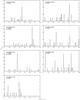 |
Fig. 1 Redshift distribution of galaxies in the group fields. The spectroscopic redshift of isolated groups is denoted by the quantity z, and for double components of bimodal groups, by zA and zB. The vertical dashed line corresponds to the redshift of the most massive component. The bin size of the histogram is δz = 0.006. |
Summary of confirmed SL2S groups.
3. Analysis and results
3.1. Redshift measurements
The spectroscopic redshifts were determined using the Radial Velocity SAO package (RVSAO; Kurtz & Mink 1998) within the IRAF software6. We first identified several emission and absorption lines by doing visual inspection of the galaxy spectra, and then we determined the redshifts by cross-correlating a spectrum against template spectra of known velocities.
The galaxy spectra cover the wavelength range 5200 Å < λ < 8400 Å, and the S/N per resolution element varies from ~5 to ~30. For most of the galaxy spectra, we were able to identify the Ca ii k+h, G-band and Mg i absorption lines, and for a few of them we also identified the Oii, Hβ, O iii, and Hα emission lines. The errors in the redshift measurements are affected by the instrumental resolution and the RVSAO template fit, and it is δz = 0.001.
The redshifts were classified into three types: secure, questionable, and unknown. Secure redshifts correspond to spectra having at least three identified lines, between absorption and emission lines; questionable redshifts to spectra having only one or two identified lines; and unknown redshifts to spectra having no identified lines. The success ratio of secure redshift determination is between 50% and 70%, which correspond to groups SL2SJ02140-0535 and SL2SJ08544-0121, respectively. We found that this ratio strongly depends on the total exposure time and magnitude of the targets.
For all the SL2S group candidates, we were able to measure the redshift of the brightest galaxy within the Einstein radius, hereafter called main lens galaxy. The spectra of the main lens galaxy of SL2S groups are shown in the top panel of the figures in Appendix A, and the main absorption and emission lines have been identified.
The galaxy redshift distributions in the direction of the SL2S group candidates are shown in Fig. 1. For five of the eight group candidates, we detected a strong peak in the redshift distribution around the redshift of the main lens galaxy.
3.2. Group membership and velocity dispersions
We adopted the formalism by Wilman et al. (2005) to determine the group membership of the SL2S systems. For the systems that showed a single peak in the redshift distribution around the redshift of the main lens galaxy, we identified the group members as follows: the group was initially assumed to be located at the redshift of the main lens galaxy, zlens, with an initial observed-frame velocity dispersion of σ(v)obs = 500(1 + zlens) km s-1. Then, we computed the maximum redshift shell, δzmax, and the maximum spatial distance, δθmax, as  where c is the speed of light, H(z) the Hubble constant at z, Dθ(z) the angular diameter distance at z, and b the axis ratio of the cylindrical linking volume. In N-body numerical simulations of dark matter halos, the cylindrical linking volume is a cylinder oriented along the line of sight with a radius equal to the projected linking length. We adopted a value of b = 3.5 in this work.
The initial guess for the velocity dispersion was based on the estimated velocity dispersion of the strong-lensing galaxy group B2108+213 measured by McKean et al. (2010). They obtained a mean value of 555 km s-1 for the galaxy group using three different linking velocity kernels. The factor (1 + zlens) is used to account for the cosmological expansion of the Universe.
Upon identifying potential members as those galaxies located inside the maximum redshift shell and the maximum projected distance, we computed the observed velocity dispersion of the group σ(v)obs. For those groups with more than ten members we used the biweight estimator (Beers et al. 1990) to compute the velocity dispersion, and for those with less than ten members we used the gapper algorithm (Beers et al. 1990). The new computed value of σ(v)obs was then used to compute new values of δzmax and δθmax. Finally, we defined the galaxies located within these limits as confirmed group members.
For the groups that showed a bimodal redshift distribution, we identified the group members of each component as follows. The first component was initially assumed to be located at the higher redshift peak, zpeak,high, with an initial observed-frame velocity dispersion of σ(v)obs = 250(1 + zpeak,high) km s-1. Then, we applied the same procedure we detailed before for groups with a single component, and finally determined the group members of the higher redshift component.
To determine the membership of the lower redshift component, we first excluded the galaxies linked to the first component. Then, we repeated the same procedure used for the first component, but this time using the lower redshift peak as a first guess.
We classified as groups those structures having at least four confirmed members in order to reduce the contamination by spurious structures in the catalogs. The final list of SL2S groups is shown in Table 2, and consists of five structures with a single component in redshift space, and two structures with a double component. The system SL2SJ02132-0743 was excluded from the group list since only two galaxies have a redshift consistent with the redshift of the main lens galaxy and also no overdensity in redshift space was found.
The group redshifts,  , and the number of spectroscopically confirmed members, Nspec, are shown in Cols. 4 and 6 of Table 2. The group redshift was computed by taking the mean of the redshift of the spectroscopically confirmed members (presented in Table B.1 of Appendix B), and then removing the peculiar motion of the Sun with respect to the CMB. To study the accuracy of the velocity dispersions and mass estimates presented in this work (see Sect. 3.3), we also computed the number of confirmed members with colors consistent with the observed E/S0 ridgeline of galaxy groups and clusters (Dressler 1984) and located inside a group-centric distance of 1 h-1 Mpc, and denoted it by Nspec,RS in Table 2.
The group velocity dispersions were estimated using the recessional velocity of their members. The measured redshift of a galaxy member, z, can be related to its peculiar velocity with respect to the group center of mass by
 where zO is the local observer O comoving with the expanding Universe, zR the cosmological redshift of the structure as measured by O relative to a comoving observer R in the vicinity of the structure, and zG the peculiar velocity of the galaxy with respect to the center of mass of the structure. The zO contribution is negligible for groups at z > 0.02.
Substituting zR by the spectroscopic redshift of the group, we obtain the following equation for the line-of-sight velocity of a galaxy with respect to the group center of mass,  (3)where
  is the group redshift as shown in Table 2.
The group velocity dispersion is related to the sum in quadrature of the vlos of all group members, and this value is affected by the recessional velocity errors. We computed the rest-frame velocity dispersion of each group by applying the biweight estimator of scale (Beers et al. 1990) to the vlos of its members. To remove the recessional velocity errors from the velocity dispersion measurements, we followed the prescription by Danese et al. (1980); i.e., we subtracted in quadrature the mean vlos errors from the velocity dispersion. The corrected line-of-sight velocity dispersions, σ(v)los, of the SL2S groups are shown in Table 2. The upper and lower errors in σ(v)los were estimated by using a bootstrap technique of 10 000 repetitions (see Beers et al. 1990, for details on the methodology).
3.3. Mass estimates
The total mass of the SL2S groups was estimated by using the virial theorem. We assumed that the groups are in hydrostatic equilibrium, have spherical symmetry, and have isotropic velocity distributions. It is important to note that the first assumption could be wrong for the youngest and least massive groups, at which the internal velocity dispersions of the galaxies are comparable to that of the group and, therefore, galaxy mergers are favored (Hickson 1997).
For distant galaxy clusters and groups, it is only possible to measure their projected velocity dispersions and galaxy separations. We computed the projected virial radius for each group using the sky angular distances between all its members, following the formalism by Girardi et al. (1998). The projected virial radius and mass were computed as  where RPV is the projected virial radius, MV the virial mass,
  the angular diameter distance at redshift z, N the number of confirmed members, θij the sky angular distance between galaxies i and j, and G the gravitational constant.
The projected virial radii and virial masses of SL2S groups are shown in Table 3, in units of Mpc and 1014 M⊙, respectively.
Virial radii and masses of SL2S groups.
4. Accuracy of velocity dispersion and mass estimates
The dynamical masses estimated for the lensed clusters can be subject to statistical and systematic biases. In this section we use GALFORM semi-analytic galaxies from the Bower et al. (2006) version of the model, which populate the Millennium simulation (Springel et al. 2005).
This simulation adopts a flat ΛCDM cosmology with z = 0 dark-matter and baryon density parameters Ωdm = 0.205, Ωb = 0.045, a dimensionless Hubble constant of h = 0.73, rms linear mass fluctuations in spheres of 8 h-1 Mpc of σ8 = 0.9, and a n = 1 slope for the primordial power spectrum. The simulation followed 21603 particles from z = 127 to z = 0 in a comoving periodic volume of 500 h-1 Mpc a side. The resulting galaxy population after applying the Bower et al. (2006) model can be considered complete down to an absolute magnitude in the r-band of Mr = −15.
To check the presence of biases in the method that was used to compute the SL2S group masses (Sect. 3.3), it is necessary to first determine the observational selection and completeness effects. The dominant selection effect is the fraction of group members that were observed and classified as secure members of each SL2S group. Coupon et al. (2009) computed the photometric redshifts for galaxies in the CFHTLS survey, and obtained a mean photometric redshift error of σz/(1 + z) ~ 0.038 and an outlier rate of η ~ 3% using a sample of 1532 galaxies (from W1 field) with secure spectroscopic redshifts. We estimated the total number of red-sequence galaxies for each group, Ngal, using a method similar to the one used by Koester et al. (2007) for building the MaxBCG cluster catalog, but we added photometric redshift information to reduce the contamination by background and foreground galaxies. We estimated Ngal for each group by counting the number of galaxies within a radius of 1 Mpc that have magnitudes brighter than R = 22.5 and colors within | g − R | < 0.24 (equivalent to 2σδ(g − R)) with respect to the E/S0 ridgeline, and have  , i.e. 1σz. We found that the number of red-sequence galaxies in the SL2S groups goes between 2 and 64 galaxies (see Table 2). The fraction of group members with measured recessional velocities was estimated as the ratio between Nspec,RS and Ngal, and it ranges from 0.25 to 0.85 (not considering the bimodal groups).
We selected halos from the z = 0.509 simulation output and repeated the observational procedure as closely as possible to measure cluster dynamical masses. The simulation cube consists of (X,Y,Z) spatial coordinates and (vX, vY, vZ) velocities. A first step consists of choosing the Z coordinate axis in the simulation cube as the line of sight and of defining the recessional velocity by Z × 100 h km s-1 Mpc-1 + vZ. Since all the groups studied in this work are bona fide gravitational lensing systems, we assume the sample to be free of spurious groups and clusters, so used the full sample of halos to do these tests.
For each individual dark-matter halo we selected galaxies in the red sequence (defined using empirical color cuts) in a cylinder with depth Δv = 500 km s-1 and width Δθ = 220″, transformed into comoving coordinates at the redshift corresponding to the selected output (z = 0.509). These values of Δv and Δθ are iteratively corrected once the velocity dispersion and harmonic projected radius of the halo are obtained from the possible members of the halo. Their final values are used to calculate the gapper mass of the halo. Figure 2 shows a comparison between the recovered and simulated masses of group-size dark matter halos (the latter being simply the number of dark-matter particles per halo multiplied by the particle mass), where it can be seen that when the member galaxies are those brighter than Mr = −18 (which corresponds to the observed i = 22 mag for a group at z ~ 0.4), the gapper method introduces important uncertainties in the recovered masses of about of 20% and 50% for masses of ~ 1014 h-1 M⊙ and ~1015h-1M⊙, respectively. We notice the significantly higher values than in the results of Biviano et al. (2006), mainly due to how few members are available in our observational samples.
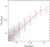 |
Fig. 2 Comparison between estimated gapper mass and underlying halo mass in the simulation. This shows the results when using a 30% of the group members brighter than Mr = −18, randomly selected. Dots represent individual measurements; the solid lines correspond to the median in bins of halo mass, and the errorbars enclose 68 percent of the individual measurements. |
A more detailed interpretation of the simulation tests is shown in Fig. 3. The top left-hand panel shows the ratio between the gapper and simulated mass of the dark matter halos as a function of the number of group members that were selected to estimate their respective group virial masses. We use the entire sample of galaxy groups from the simulation, and on average the number of members is 60. As can be seen, the statistical errors shown by the error bars (enclosing 68 percent of the individual results) is significantly larger than the systematic bias. In the case of the larger sample of galaxies (selected with Mr < −18), the bias is almost zero, with a slight tendency to recover a lower value for the estimated mass as the fraction increases. The same conclusion applies for the analysis using the brighter sample of members, with the difference that, regardless of the fraction of members used in the analysis, the estimated group masses are always lower than their simulated counterparts. It is interesting to note that biases in the mass estimates are lower than 20 percent for all the cases, and that their error bars decrease as the fraction of group members used in the calculation of the mass approaches 20%. We emphasize that the average number of true members is constant across the x-axis; i.e., we only change the number of spectroscopic members used to estimate the group mass. The top right-hand panel shows the mass ratio as a function of the total number of members, which spans between 20 and 300 members on average. As discussed in Sect. 2, the mean fraction of group members with spectroscopic measurements for the SL2S groups is about 30%; as can be seen, using a larger fraction would not have resulted in much of an improvement (and would require significantly more telescope time).
To account for the sources of uncertainty in the estimation of the virial mass, in the bottom left-hand panel of Fig. 3, we show the ratio between the group velocity dispersions estimated by using the gapper method and the ones obtained from the full numerical simulation. In the bottom right-hand panel, we show the ratio between the estimated harmonic radii, rgap, and the average 3D radii of simulated dark matter halos, r3D. Our results suggest that the velocity dispersion is always underestimated and that it gets closer to the underlying value as the fraction of observed group members increases (with little change above a fraction of 0.3). Furthermore, we found that the virial radius is also underestimated, and it departs from the actual value as the fraction of members increases. We note that the ratio rgap/r3D cannot be compared with the ratios in columns 9 and 10 of Table 1 from Biviano et al. (2006), since we use a different method to estimate the virial radius.
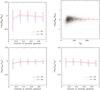 |
Fig. 3 Top left: ratio between the estimated and actual masses of group-size dark matter haloes as a function of the fraction of group members with recessional velocity measurements, as obtained from the numerical simulations presented in this work. Top right: ratio between the estimated and actual masses of group-size dark matter haloes as a function of the number of member galaxies. Bottom left: ratio between the velocity dispersion as estimated with the gapper method and as obtained from the actual group members in the simulation. Bottom right: ratio between the deprojected virial radius and the mean 3D radius of actual groups members in the simulation, as a function of the fraction of members. The solid red lines show the results when using only members with absolute magnitudes brighter than Mr = −18, and the dotted blue lines for members brighter than Mr = −19. Errorbars enclose 68% of the measurements in each bin of fraction. |
The previous tests were applied to bound systems with masses higher than 1014 M⊙, but could also be applied to a subset of simulated groups of masses similar to any of the observed SL2S groups. We chose the group SL2SJ02140-0535 as a particular case for applying the test, since this group has the largest number of confirmed members and a virial mass properly covered by the numerical simulation (Verdugo et al. 2011). We selected halos from the numerical simulation with velocity dispersions within a narrow range around the measured value for SL2SJ02140-0535 (264 < σ(v)los < 464 km s-1), and restricted to halos having a total number of Mr < −21 galaxies between 20 and 40, which brackets the estimated number of members for this group. The main aim of studying this restricted sample of groups was to obtain the systematic and statistical uncertainties in the estimated mass of SL2SJ02140-0535. The ratio between the estimated and actual masses for this subsample of halos is shown in Fig. 4, where as can be seen, when using galaxies brighter than Mr = −18 the resulting biases are comparable to those found for the full sample of halos in the numerical simulation.
The main conclusions are that the expected biases in the virial mass estimation are lower than the statistical uncertainties of group properties in a narrow range of mass and that the virial mass is underestimated by about 15% when using 30% of the group members. According to Fig. 4, the bias appears to worsen for higher fractions of members, but this effect is likely due to the small sample of halos resulting from the cuts applied to mimic SL2SJ02140-0535.
5. Discussion
The formation and evolution history of galaxies has been shown to strongly depends on the properties of the environment they inhabit. The existence of this environmental dependance has been confirmed both in the local (Goto et al. 2003; Helsdon & Ponman 2003; Bamford et al. 2009) and intermediate redshift Universe (Dressler et al. 1997; Treu et al. 2003; Pannella et al. 2009), and the observational results suggest that star formation and galaxy merging processes are accelerated in high density environments, such as galaxy groups and clusters.
Therefore, galaxy groups represent natural laboratories for studying the relative importance of the different astrophysical processes occurring in dense regions of the Universe. For instance, galaxy collisions are expected to be most effective in groups because the dynamical friction timescale is similar to the orbital timescale of galaxies within the group. Since galaxy groups contain a low number of members (less than one hundred within 1 Mpc) and cover a wide range in mass, velocity dispersion and hot gas content, it is necessary to characterize their properties in detail in order to build representative samples of groups and to properly study the relative importance of the different mechanisms.
The virial mass estimation relies on the following assumptions: sphericity, kinematic isotropy and virialization. In our virial mass estimation we use the velocity dispersion, which we assume constant through the group, and the harmonic radius as an estimate of the virial radius (see Sect. 3.1). These assumptions depart slightly from observational results. For instance, i) groups and clusters usually show substructure (Riemer-Sørensen et al. 2009); ii) it is known that nearby clusters show a small gradient in the velocity dispersion (Kent & Gunn 1982); and iii) some groups at high redshift show evidence of having merging events, and therefore are not in a virialized state (McKean et al. 2010). Furthermore, it is well known that the harmonic radius depends strongly on the area covered by the spectroscopic observations and the number of confirmed members (Biviano et al. 2006; Girardi et al. 1998), biasing the measurement of the virial radius. From our simulations, it seems that the virial radius is underestimated when the number of members increases, contrary to the results obtained by Biviano et al. (2006). The difference between our results and those from Biviano et al. (2006) could be explained by the differences in the simulations, since the latter uses an N-body hydrodynamical simulation.
We ran numerical simulations to assess the bias introduced in the virial mass estimation (see Sect. 4). The results show that the method adopted in this work allows to recovering the mass of the simulated groups within the error bars, showing no systematic deviations (see top panel of Fig. 3). It is also important to note that i) the mass estimation of a group with 40% of their members observed is as good as when using 90% of the members; ii) the mass estimation improves with the number of groups used and justifies the stacking of groups of similar properties in order to obtain better estimations. However, for the particular case in which we applied a cut in velocity dispersion, the case of SL2SJ02140-0535, the simulation shows that the method underestimates the group mass by about 20% (see Fig. 4). The analysis of simulated groups selected from the numerical simulations (see Sect. 4 and Fig. 3) reveals that the virial mass of the SL2S groups is underestimated by 15%.
Limousin et al. (2009) computed the weak lensing velocity dispersions and masses for several of the SL2S systems studied in this work. The mass estimate obtained from weak lensing measurements makes no assumption regarding the dynamic state of the systems, as opposed to the kinematical measurements presented in this work. Although weak lensing requires less assumptions, it has been shown that the estimated mass of galaxy clusters can be strongly affected by intervening large-scale structure along its line of sight (Hoekstra et al. 2011).
Figure 5 shows the line-of-sight velocity dispersions as estimated from dynamics and weak lensing measurements for the groups SL2SJ02140-0535, SL2SJ02215-0647, SL2SJ08544-0121, and SL2SJ09413-1100. We found that weak lensing estimates are systematically larger by 50% than dynamical estimates. This is in stark contrast to measurements from galaxy-galaxy lensing by SLACS (Treu et al. 2006a,b), where the ratio between the central stellar velocity dispersion and the velocity dispersion that best fit the lensing model is 1.01 ± 0.02. Although numerical simulations (see Sect. 4) suggest that the viral mass is underestimated by 20%, this is not enough to explain the inferred discrepancy. Thus, our results may indicate that the isothermal sphere model is not a good assumption for galaxy groups.
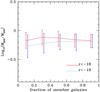 |
Fig. 4 Ratio between the estimated and actual masses of simulated groups with total number of members and velocity dispersions similar to the ones measured for SL2SJ02140-0535, i.e. number of members between 20 and 40, and velocity dispersion between 260 and 460 km s-1. The number of groups in each bin of the plot remains constant. The x-axis corresponds to the fraction of members used for calculating the group mass. |
6. Conclusions
This paper presents the spectroscopic follow-up and dynamical analysis of eight group candidates identified in the SL2S survey. Our analysis reveals that seven of the systems correspond to gravitationally bound structures, where five have a single component in redshift-space and two have a double component (bimodal galaxy distribution). They span a wide range in redshift between 0.35 and 0.65, and a wide range in mass between 5 × 10¹³ M⊙ and 1.5 × 10¹⁴ M⊙.
The main results of this paper are given as follows:
-
1.
The success rate of the spectroscopic confirmation of groupsidentified in the SL2S survey is about 88%. It is similar to thesuccess rate of clusters followed-up in the Red-Sequence ClusterSurvey (RCS-1; Gladders &Yee 2005).
-
2.
We find that weak lensing estimates of the group velocity dispersions are 50% greater than dynamical estimates. This discrepancy has been never reported before by other studies of groups and clusters, and is in stark contrast to measurements from galaxy-galaxy lensing.
-
3.
From numerical simulations, we concluded that measuring redshifts for only 30% of the total galaxy population in groups is enough to recover the group velocity dispersion with less than 5% systematic error.
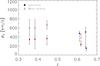 |
Fig. 5 Velocity dispersion of SL2S groups as estimated from galaxy dynamics (solid circles) and weak lensing measurements (open triangles). The red symbols show the groups with dynamical and weak lensing estimates, while blue symbols those groups with only dynamical estimates. Only one group at z > 0.6 has enough weak lensing signal to estimate an upper limit to its velocity dispersion. |
Online material
Appendix A: Presentation of each group
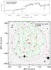 |
Fig. A.1 Top panel: optical spectra of the brightest confirmed member of SL2SJ02140-0535. The main absorption lines used to determine the redshift of the main lens galaxy have been identified. Bottom panel: spatial distribution of galaxies in the group field of SL2SJ02140-0535. Red rectangles show the position of the spectroscopically confirmed members. The dashed magenta circle shows a circular aperture of radius 1 Mpc at z = 0.44. The contours in green show the luminosity contours equal to 3 × 10⁵, 106, 3 × 10⁶ and 107 L⊙ kpc-2 from outermost to innermost, as computed by Limousin et al. (2009). |
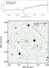 |
Fig. A.2 Top panel: optical spectra of the brightest confirmed member of SL2SJ02141-0405. The main absorption and emission lines used to determine the redshift of the main lens galaxy have been identified. Bottom panel: spatial distribution of galaxies in the group field of SL2SJ02141-0405. Red rectangles show the position of the spectroscopically confirmed members. The dashed magenta circle shows a circular aperture of radius 1 Mpc at z = 0.61. The contours are the same as in Fig. A.1. |
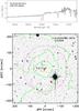 |
Fig. A.3 Top panel: optical spectra of the brightest confirmed member of SL2SJ02180-0515. The main absorption lines used to determine the redshift of the main lens galaxy have been identified. Bottom panel: spatial distribution of galaxies in the group field of SL2SJ02180-0515. Red rectangles show the position of the spectroscopically confirmed members. The dashed magenta circle shows a circular aperture of radius 1 Mpc at z = 0.64. The contours are the same as in Fig. A.1. |
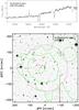 |
Fig. A.4 Top panel: optical spectra of the brightest confirmed member of SL2SJ02215-0647. The main absorption and emission lines used to determine the redshift of the main lens galaxy have been identified. Bottom panel: spatial distribution of galaxies in the group field of SL2SJ02215-0647. Red rectangles show the position of the spectroscopically confirmed members. The dashed magenta circle shows a circular aperture of radius 1 Mpc at z = 0.62. The contours are the same as in Fig. A.1. |
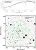 |
Fig. A.5 Top panel: optical spectra of the brightest confirmed member of SL2SJ08544-0121. The main absorption lines used to determine the redshift of the main lens galaxy have been identified. Bottom panel: spatial distribution of galaxies in the group field of SL2SJ08544-0121. Red rectangles show the position of the spectroscopically confirmed members. The dashed magenta circle shows a circular aperture of radius 1 Mpc at z = 0.35. The contours are the same as in Fig. A.1. |
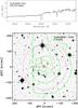 |
Fig. A.6 Top panel: optical spectra of the brightest confirmed member of SL2SJ08591-0345. The main absorption lines used to determine the redshift of the main lens galaxy have been identified. Bottom panel: spatial distribution of galaxies in the group field of SL2SJ08591-0345. Red rectangles show the position of the spectroscopically confirmed members. The dashed magenta circle shows a circular aperture of radius 1 Mpc at z = 0.64. The contours are the same as in Fig. A.1. |
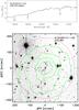 |
Fig. A.7 Top panel: optical spectra of the brightest confirmed member of SL2SJ09413-1100. The main absorption lines used to determine the redshift of the main lens galaxy have been identified. Bottom panel: spatial distribution of galaxies in the group field of SL2SJ09413-1100. Red rectangles show the position of the spectroscopically confirmed members. The dashed magenta circle shows a circular aperture of radius 1 Mpc at z = 0.39. The contours are the same as in Fig. A.1. |
Appendix B: Summary of FORS2 masks and spectroscopic confirmed members for each group
Summary of group members.
Very Large Telescope Paranal Science Operations FORS data reduction cookbook, v1
IRAF is distributed by the National Optical Astronomy Observatories, which are operated by the Association of Universities for Research in Astronomy, Inc., under cooperative agreement with the National Science Foundation.
Acknowledgments
We thank Ricardo Salinas and Anupreeta More for enlightening conversations. We thank the referee for the useful and constructive comments to improve this paper. The authors acknowledge support from Fondo ALMA-CONICYT N° 31090019, Comité Mixto ESO-Gobierno de Chile, FONDECYT through grant 1090637 and Programme National de Cosmologie (PNCG). R.P. Muñoz acknowledges support from CONICYT CATA-BASAL and FONDECYT through grant 3130750. V. Motta gratefully acknowledges support from FONDECYT through grant 1090673 and 1120741. T. Verdugo acknowledges support from FONDECYT through grant 3090025 and CONACYT through grant 165365. M. Limousin acknowledges the Centre National de la Recherche Scientifique for its support and the Dark Cosmology Centre is funded by the Danish National Research Foundation. N. Padilla acknowledges support from FONDAP “Center for Astrophysics”, CONICYT CATA-BASAL and FONDECYT through grant 1110328. G. Foëx acknowledges support from FONDECYT through grant 3120160. R. Gavazzi acknowledges support from the Centre National des Études Spatiales. This work made use of the Geryon cluster at the Centro de Astro-Ingeniería UC.
References
- Abazajian, K., Adelman-McCarthy, J. K., Agüeros, M. A., et al. 2004, AJ, 128, 502 [Google Scholar]
- Adami, C., Mazure, A., Ilbert, O., et al. 2005, A&A, 443, 805 [NASA ADS] [CrossRef] [EDP Sciences] [Google Scholar]
- Alard, C. 2006 [arXiv:astro-ph/0606757] [Google Scholar]
- Appenzeller, I., Fricke, K., Fürtig, W., et al. 1998, The Messenger, 94, 1 [NASA ADS] [Google Scholar]
- Bamford, S. P., Nichol, R. C., Baldry, I. K., et al. 2009, MNRAS, 393, 1324 [NASA ADS] [CrossRef] [Google Scholar]
- Beers, T. C., Flynn, K., & Gebhardt, K. 1990, AJ, 100, 32 [NASA ADS] [CrossRef] [Google Scholar]
- Berlind, A. A., Frieman, J., Weinberg, D. H., et al. 2006, ApJS, 167, 1 [NASA ADS] [CrossRef] [Google Scholar]
- Biviano, A., Murante, G., Borgani, S., et al. 2006, A&A, 456, 23 [NASA ADS] [CrossRef] [EDP Sciences] [Google Scholar]
- Bower, R. G., Benson, A. J., Malbon, R., et al. 2006, MNRAS, 370, 645 [NASA ADS] [CrossRef] [Google Scholar]
- Brough, S., Forbes, D. A., Kilborn, V. A., & Couch, W. 2006, MNRAS, 370, 1223 [NASA ADS] [CrossRef] [Google Scholar]
- Cabanac, R. A., Alard, C., Dantel-Fort, M., et al. 2007, A&A, 461, 813 [NASA ADS] [CrossRef] [EDP Sciences] [Google Scholar]
- Churazov, E., Brüggen, M., Kaiser, C. R., Böhringer, H., & Forman, W. 2001, ApJ, 554, 261 [NASA ADS] [CrossRef] [Google Scholar]
- Colless, M., Dalton, G., Maddox, S., et al. 2001, MNRAS, 328, 1039 [NASA ADS] [CrossRef] [Google Scholar]
- Coupon, J., Ilbert, O., Kilbinger, M., et al. 2009, A&A, 500, 981 [NASA ADS] [CrossRef] [EDP Sciences] [Google Scholar]
- Danese, L., de Zotti, G., & di Tullio, G. 1980, A&A, 82, 322 [NASA ADS] [Google Scholar]
- Davis, M., Faber, S. M., Newman, J., et al. 2003, in SPIE Conf. 4834, ed. P. Guhathakurta, 161 [Google Scholar]
- Dressler, A. 1984, ARA&A, 22, 185 [Google Scholar]
- Dressler, A., Oemler, Jr., A., Couch, W. J., et al. 1997, ApJ, 490, 577 [NASA ADS] [CrossRef] [Google Scholar]
- Eke, V. R., Baugh, C. M., Cole, S., et al. 2004, MNRAS, 348, 866 [NASA ADS] [CrossRef] [Google Scholar]
- Finoguenov, A., Connelly, J. L., Parker, L. C., et al. 2009, ApJ, 704, 564 [NASA ADS] [CrossRef] [Google Scholar]
- Geller, M. J., & Huchra, J. P. 1983, ApJS, 52, 61 [NASA ADS] [CrossRef] [Google Scholar]
- Gerke, B. F., Newman, J. A., Davis, M., et al. 2005, ApJ, 625, 6 [NASA ADS] [CrossRef] [Google Scholar]
- Girardi, M., Giuricin, G., Mardirossian, F., Mezzetti, M., & Boschin, W. 1998, ApJ, 505, 74 [NASA ADS] [CrossRef] [Google Scholar]
- Gladders, M. D., & Yee, H. K. C. 2005, ApJS, 157, 1 [NASA ADS] [CrossRef] [Google Scholar]
- Goto, T., Yamauchi, C., Fujita, Y., et al. 2003, MNRAS, 346, 601 [NASA ADS] [CrossRef] [Google Scholar]
- Hansen, S. M., Sheldon, E. S., Wechsler, R. H., & Koester, B. P. 2009, ApJ, 699, 1333 [NASA ADS] [CrossRef] [Google Scholar]
- Helsdon, S. F., & Ponman, T. J. 2003, MNRAS, 339, L29 [NASA ADS] [CrossRef] [Google Scholar]
- Hickson, P. 1997, ARA&A, 35, 357 [NASA ADS] [CrossRef] [Google Scholar]
- Hoekstra, H., Hartlap, J., Hilbert, S., & van Uitert, E. 2011, MNRAS, 412, 2095 [NASA ADS] [CrossRef] [Google Scholar]
- Horne, K. 1986, PASP, 98, 609 [NASA ADS] [CrossRef] [EDP Sciences] [Google Scholar]
- Kent, S. M., & Gunn, J. E. 1982, AJ, 87, 945 [NASA ADS] [CrossRef] [Google Scholar]
- Knobel, C., Lilly, S. J., Iovino, A., et al. 2012, ApJ, 753, 121 [NASA ADS] [CrossRef] [Google Scholar]
- Koester, B. P., McKay, T. A., Annis, J., et al. 2007, ApJ, 660, 221 [NASA ADS] [CrossRef] [Google Scholar]
- Kurtz, M. J., & Mink, D. J. 1998, PASP, 110, 934 [NASA ADS] [CrossRef] [Google Scholar]
- Lilly, S. J., Le Fèvre, O., Renzini, A., et al. 2007, ApJS, 172, 70 [NASA ADS] [CrossRef] [Google Scholar]
- Limousin, M., Cabanac, R., Gavazzi, R., et al. 2009, A&A, 502, 445 [NASA ADS] [CrossRef] [EDP Sciences] [Google Scholar]
- Marinoni, C., Davis, M., Newman, J. A., & Coil, A. L. 2002, ApJ, 580, 122 [NASA ADS] [CrossRef] [Google Scholar]
- McCarthy, I. G., Schaye, J., Ponman, T. J., et al. 2010, MNRAS, 406, 822 [NASA ADS] [Google Scholar]
- McKean, J. P., Auger, M. W., Koopmans, L. V. E., et al. 2010, MNRAS, 404, 749 [NASA ADS] [CrossRef] [Google Scholar]
- Mihos, J. C., & Hernquist, L. 1996, ApJ, 464, 641 [NASA ADS] [CrossRef] [Google Scholar]
- More, A., Cabanac, R., More, S., et al. 2012, ApJ, 749, 38 [Google Scholar]
- Oemler, Jr., A. 1974, ApJ, 194, 1 [NASA ADS] [CrossRef] [Google Scholar]
- Oguri, M. 2006, MNRAS, 367, 1241 [NASA ADS] [CrossRef] [Google Scholar]
- Padilla, N., Lambas, D. G., & González, R. 2010, MNRAS, 409, 936 [NASA ADS] [CrossRef] [Google Scholar]
- Pannella, M., Gabasch, A., Goranova, Y., et al. 2009, ApJ, 701, 787 [NASA ADS] [CrossRef] [Google Scholar]
- Riemer-Sørensen, S., Paraficz, D., Ferreira, D. D. M., et al. 2009, ApJ, 693, 1570 [NASA ADS] [CrossRef] [Google Scholar]
- Springel, V., White, S. D. M., Jenkins, A., et al. 2005, Nature, 435, 629 [NASA ADS] [CrossRef] [PubMed] [Google Scholar]
- Treu, T., Ellis, R. S., Kneib, J.-P., et al. 2003, ApJ, 591, 53 [NASA ADS] [CrossRef] [Google Scholar]
- Treu, T., Koopmans, L. V., Bolton, A. S., Burles, S., & Moustakas, L. A. 2006a, ApJ, 640, 662 [NASA ADS] [CrossRef] [Google Scholar]
- Treu, T., Koopmans, L. V. E., Bolton, A. S., Burles, S., & Moustakas, L. A. 2006b, ApJ, 650, 1219 [NASA ADS] [CrossRef] [Google Scholar]
- Verdugo, T., Motta, V., Muñoz, R. P., et al. 2011, A&A, 527, A124 [NASA ADS] [CrossRef] [EDP Sciences] [Google Scholar]
- Wilman, D. J., Balogh, M. L., Bower, R. G., et al. 2005, MNRAS, 358, 71 [NASA ADS] [CrossRef] [Google Scholar]
- Yang, X., Mo, H. J., van den Bosch, F. C., et al. 2007, ApJ, 671, 153 [NASA ADS] [CrossRef] [Google Scholar]
- York, D. G., Adelman, J., Anderson, Jr., J. E., et al. 2000, AJ, 120, 1579 [Google Scholar]
- Zapata, T., Perez, J., Padilla, N., & Tissera, P. 2009, MNRAS, 394, 2229 [NASA ADS] [CrossRef] [Google Scholar]
All Tables
All Figures
|
Fig. 1 Redshift distribution of galaxies in the group fields. The spectroscopic redshift of isolated groups is denoted by the quantity z, and for double components of bimodal groups, by zA and zB. The vertical dashed line corresponds to the redshift of the most massive component. The bin size of the histogram is δz = 0.006. |
| In the text | |
|
Fig. 2 Comparison between estimated gapper mass and underlying halo mass in the simulation. This shows the results when using a 30% of the group members brighter than Mr = −18, randomly selected. Dots represent individual measurements; the solid lines correspond to the median in bins of halo mass, and the errorbars enclose 68 percent of the individual measurements. |
| In the text | |
|
Fig. 3 Top left: ratio between the estimated and actual masses of group-size dark matter haloes as a function of the fraction of group members with recessional velocity measurements, as obtained from the numerical simulations presented in this work. Top right: ratio between the estimated and actual masses of group-size dark matter haloes as a function of the number of member galaxies. Bottom left: ratio between the velocity dispersion as estimated with the gapper method and as obtained from the actual group members in the simulation. Bottom right: ratio between the deprojected virial radius and the mean 3D radius of actual groups members in the simulation, as a function of the fraction of members. The solid red lines show the results when using only members with absolute magnitudes brighter than Mr = −18, and the dotted blue lines for members brighter than Mr = −19. Errorbars enclose 68% of the measurements in each bin of fraction. |
| In the text | |
|
Fig. 4 Ratio between the estimated and actual masses of simulated groups with total number of members and velocity dispersions similar to the ones measured for SL2SJ02140-0535, i.e. number of members between 20 and 40, and velocity dispersion between 260 and 460 km s-1. The number of groups in each bin of the plot remains constant. The x-axis corresponds to the fraction of members used for calculating the group mass. |
| In the text | |
|
Fig. 5 Velocity dispersion of SL2S groups as estimated from galaxy dynamics (solid circles) and weak lensing measurements (open triangles). The red symbols show the groups with dynamical and weak lensing estimates, while blue symbols those groups with only dynamical estimates. Only one group at z > 0.6 has enough weak lensing signal to estimate an upper limit to its velocity dispersion. |
| In the text | |
|
Fig. A.1 Top panel: optical spectra of the brightest confirmed member of SL2SJ02140-0535. The main absorption lines used to determine the redshift of the main lens galaxy have been identified. Bottom panel: spatial distribution of galaxies in the group field of SL2SJ02140-0535. Red rectangles show the position of the spectroscopically confirmed members. The dashed magenta circle shows a circular aperture of radius 1 Mpc at z = 0.44. The contours in green show the luminosity contours equal to 3 × 10⁵, 106, 3 × 10⁶ and 107 L⊙ kpc-2 from outermost to innermost, as computed by Limousin et al. (2009). |
| In the text | |
|
Fig. A.2 Top panel: optical spectra of the brightest confirmed member of SL2SJ02141-0405. The main absorption and emission lines used to determine the redshift of the main lens galaxy have been identified. Bottom panel: spatial distribution of galaxies in the group field of SL2SJ02141-0405. Red rectangles show the position of the spectroscopically confirmed members. The dashed magenta circle shows a circular aperture of radius 1 Mpc at z = 0.61. The contours are the same as in Fig. A.1. |
| In the text | |
|
Fig. A.3 Top panel: optical spectra of the brightest confirmed member of SL2SJ02180-0515. The main absorption lines used to determine the redshift of the main lens galaxy have been identified. Bottom panel: spatial distribution of galaxies in the group field of SL2SJ02180-0515. Red rectangles show the position of the spectroscopically confirmed members. The dashed magenta circle shows a circular aperture of radius 1 Mpc at z = 0.64. The contours are the same as in Fig. A.1. |
| In the text | |
|
Fig. A.4 Top panel: optical spectra of the brightest confirmed member of SL2SJ02215-0647. The main absorption and emission lines used to determine the redshift of the main lens galaxy have been identified. Bottom panel: spatial distribution of galaxies in the group field of SL2SJ02215-0647. Red rectangles show the position of the spectroscopically confirmed members. The dashed magenta circle shows a circular aperture of radius 1 Mpc at z = 0.62. The contours are the same as in Fig. A.1. |
| In the text | |
|
Fig. A.5 Top panel: optical spectra of the brightest confirmed member of SL2SJ08544-0121. The main absorption lines used to determine the redshift of the main lens galaxy have been identified. Bottom panel: spatial distribution of galaxies in the group field of SL2SJ08544-0121. Red rectangles show the position of the spectroscopically confirmed members. The dashed magenta circle shows a circular aperture of radius 1 Mpc at z = 0.35. The contours are the same as in Fig. A.1. |
| In the text | |
|
Fig. A.6 Top panel: optical spectra of the brightest confirmed member of SL2SJ08591-0345. The main absorption lines used to determine the redshift of the main lens galaxy have been identified. Bottom panel: spatial distribution of galaxies in the group field of SL2SJ08591-0345. Red rectangles show the position of the spectroscopically confirmed members. The dashed magenta circle shows a circular aperture of radius 1 Mpc at z = 0.64. The contours are the same as in Fig. A.1. |
| In the text | |
|
Fig. A.7 Top panel: optical spectra of the brightest confirmed member of SL2SJ09413-1100. The main absorption lines used to determine the redshift of the main lens galaxy have been identified. Bottom panel: spatial distribution of galaxies in the group field of SL2SJ09413-1100. Red rectangles show the position of the spectroscopically confirmed members. The dashed magenta circle shows a circular aperture of radius 1 Mpc at z = 0.39. The contours are the same as in Fig. A.1. |
| In the text | |
Current usage metrics show cumulative count of Article Views (full-text article views including HTML views, PDF and ePub downloads, according to the available data) and Abstracts Views on Vision4Press platform.
Data correspond to usage on the plateform after 2015. The current usage metrics is available 48-96 hours after online publication and is updated daily on week days.
Initial download of the metrics may take a while.