| Issue |
A&A
Volume 552, April 2013
|
|
|---|---|---|
| Article Number | A119 | |
| Number of page(s) | 20 | |
| Section | Planets and planetary systems | |
| DOI | https://doi.org/10.1051/0004-6361/201118179 | |
| Published online | 11 April 2013 | |
Magnetic energy fluxes in sub-Alfvénic planet star and moon planet interactions⋆
1
Institut für Geophysik und Meteorologie, Universität zu Köln,
Cologne,
Germany
e-mail: This email address is being protected from spambots. You need JavaScript enabled to view it.
; This email address is being protected from spambots. You need JavaScript enabled to view it.
;
This email address is being protected from spambots. You need JavaScript enabled to view it.
; This email address is being protected from spambots. You need JavaScript enabled to view it.
2
1. Physikalisches Institut, Universität zu Köln,
Cologne,
Germany
e-mail: This email address is being protected from spambots. You need JavaScript enabled to view it.
Received:
29
September
2011
Accepted:
2
January
2013
Abstract
Context. Electromagnetic coupling of planetary moons with their host planets is well observed in our solar system. Similar couplings of extrasolar planets with their central stars have been studied observationally on an individual as well as on a statistical basis.
Aims. We aim to model and to better understand the energetics of planet star and moon planet interactions on an individual and as well as on a statistical basis.
Methods. We derived analytic expressions for the Poynting flux communicating magnetic field energy from the planetary obstacle to the central body for sub-Alfvénic interaction. We additionally present simplified, readily useable approximations for the total Poynting flux for small Alfvén Mach numbers. These energy fluxes were calculated near the obstacles and thus likely present upper limits for the fluxes arriving at the central body. We applied these expressions to satellites of our solar system and to HD 179949 b. We also performed a statistical analysis for 850 extrasolar planets.
Results. Our derived Poynting fluxes compare well with the energetics and luminosities of the satellites’ footprints observed at Jupiter and Saturn. We find that 295 of 850 extrasolar planets are possibly subject to sub-Alfvénic plasma interactions with their stellar winds, but only 258 can magnetically connect to their central stars due to the orientations of the associated Alfvén wings. The total energy fluxes in the magnetic coupling of extrasolar planets vary by many orders of magnitude and can reach values larger than 1019 W. Our calculated energy fluxes generated at HD 179949 b can only explain the observed energy fluxes for exotic planetary and stellar magnetic field properties. In this case, additional energy sources triggered by the Alfvén wave energy launched at the extrasolar planet might be necessary. We provide a list of extrasolar planets where we expect planet star coupling to exhibit the largest energy fluxes. As supplementary information we also attach a table of the modeled stellar wind plasma properties and possible Poynting fluxes near all 850 extrasolar planets included in our study.
Conclusions. The orders of magnitude variations in the values for the total Poynting fluxes even for close-in extrasolar planets provide a natural explanation why planet star coupling might have been only observable on an individual basis but not on a statistical basis.
Key words: planet-star interactions / planets and satellites: general / planets and satellites: magnetic fields
Estimated plasma parameters and their associated Poynting fluxes are only available at the CDS via anonymous ftp to cdsarc.u-strasbg.fr (130.79.128.5) or via http://cdsarc.u-strasbg.fr/viz-bin/qcat?J/A+A/552/A119
© ESO, 2013
1. Introduction
Planetary bodies throughout the universe are commonly embedded in a flow of magnetized plasma. These bodies are thereby obstacles to the flow and interact with their surrounding plasma. Among the different types of waves excited in these interactions, the Alfvén mode is particularly important because it can transport energy and momentum along the local background magnetic field with very little dispersion over large distances. An interesting case of this interaction occurs if the relative velocity v0 between the plasma and the obstacle is smaller than the Alfvén velocity vA, i.e. the Alfvén Mach number MA = v0/vA is smaller than 1. Then a necessary condition is met that the Alfvén mode can carry energy and momentum in the upstream direction of the flow.
Sub-Alfvénic plasma interaction (MA < 1) is well known in our solar system. It has been observed and studied for artificial satellites in the Earth’s magnetosphere (Drell et al. 1965). It is also common in the outer solar system, where the planetary satellites are often close enough to their parent planets such that their orbits are within the planets’ magnetospheres. In these cases the relative velocities between the planetary satellites and the magnetospheric plasma are often small enough for the plasma interaction to be sub-Alfvénic. Historically, the interaction of Io with Jupiter’s magnetosphere played the leading role in advancing, both observationally and theoretically, our understanding of sub-Alfvénic plasma interaction. Io’s interaction has been observed through its control of Jupiter’s radio waves (e.g., Bigg 1964; Zarka 1998), by in-situ measurements of the Voyager and Galileo spacecraft (e.g., Acuña et al. 1981; Kivelson et al. 1996b; Frank et al. 1996), and subsequently as Io’s footprints in Jupiter’s atmosphere (Connerney et al. 1993; Prangé et al. 1996; Clarke et al. 1996; Bonfond et al. 2008; Wannawichian et al. 2010; Bonfond 2012; Bonfond et al. 2013). In conjunction with the observational progress, the electrodynamic coupling between Io and Jupiter has been extensively studied theoretically and numerically as well (e.g., Piddington & Drake 1968; Goldreich & Lynden-Bell 1969; Neubauer 1980; Goertz 1980; Wright & Schwartz 1989; Jacobsen et al. 2007, 2010). Next to Io, sub-Alfvénic satellite interactions with significant energy exchanges have also been observed at Jupiter’s large satellites Europa, Ganymede and Callisto (Kivelson et al. 2004) and imprints of the interaction in Jupiter’s atmosphere in form of auroral footprints have been observed for Europa and Ganymede (Clarke et al. 2002; Grodent et al. 2006, 2009; Bonfond 2012). Hints for a Callisto footprint have been reported by Clarke et al. (2011). Recently, Cassini spacecraft observations identified a significant sub-Alfvénic interaction at Saturn’s satellite Enceladus generated by geyser activity near its south pole (Dougherty et al. 2006; Tokar et al. 2006; Khurana et al. 2007; Saur et al. 2007, 2008; Kriegel et al. 2009; 2011; Jia et al. 2010; Simon et al. 2011a). The Alfvén waves launched near Enceladus also generate footprints in Saturn’s upper atmosphere as recently discovered (Pryor et al. 2011).
In our own solar system, all planets are sufficiently far away from the sun such that the relative velocity between the solar wind and the planets is super-Alfvénic (MA > 1) and super-fast nearly all the time, i.e. the relative plasma velocity is larger than the group velocity of the fast magneto-sonic mode. In our solar system MA = 1 occurs on average around 0.08 AU and Mercury’s perihelion is near 0.31 AU. Chané et al. (2012) recently reported an exceptional period where the solar wind upstream from Earth was sub-Alfvénic for a time period of four hours. During that time period the Earth lost its bow shock and developed Alfvén wings. The Alfvén wings were, however, not able to connect to our sun because the sub-Alfvénic period lasted not long enough. Many of the extrasolar planets discovered so far orbit their central stars within close distances, i.e. less than 0.1 AU. At close radial distance, the stellar wind likely often has not reached a flow speed which exceeds the Alfvén velocity. Thus the interaction is sub-Alfvénic and Alfvén waves generated by the interaction can travel upstream and transport energy to the central star when the orientation of the stellar wind magnetic field is favorable (as described in detail in this work). Similar sub-Alfvénic interactions occur in our solar system between planetary satellites and their central planets. The resulting sub-Alfvénic plasma interaction does not generate a bow-shock, but an Alfvén wing structure in the satellites/planets plasma environment. The interaction of extrasolar planets with their central star is commonly called star-planet interaction (SPI) in the literature (e.g., Shkolnik et al. 2003).
Observational evidence for such a magnetic extrasolar planet star coupling comes from measurements of enhanced stellar Ca emission correlated with the orbital periods of close in extrasolar planets by Shkolnik et al. (2003, 2005, 2008). In particular for HD 179949, the synchronicity of the Ca emission with the orbital period is visible in four out of six epochs (Shkolnik et al. 2008). For this star, Shkolnik et al. (2005) estimate a chromospheric excess energy flux of ~1020 Watt, i.e. the same order of magnitude as a typical flare.
Next to individual studies, SPI is also investigated on a statistical basis. Scharf (2010) presents an analysis of X-ray fluxes from extrasolar planet harboring stars and argues that stars with extrasolar planets closer than 0.15 AU show a correlation of X-ray flux with the mass of the extrasolar planets, while extrasolar planets at larger distances show no correlation. Poppenhaeger et al. (2010) also provide a statistical analysis of X-ray fluxes from a sample of 72 stars, which host extrasolar planets, but arrive at a different conclusion compared to Scharf (2010). The authors show that there are no significant correlations of the normalized X-ray flux with planetary mass or semi-major axis. Thus Poppenhaeger et al. (2010) see no statistical evidence of SPI even though SPI might still be observable for some individual targets. In their most recent study Poppenhaeger & Schmitt (2011) argue that the correlation derived in Scharf (2010) is caused by selection effects and does not trace possible planet induced phenomena in stellar coronae. In another study in the υ Andromedae system, Poppenhaeger et al. (2011) also find no evidence in X-rays or in the optical that can be identified being due to extrasolar planets.
Theoretical aspects of the plasma interaction at extrasolar planets have been addressed by a series of authors. Cuntz et al. (2000) estimate with simplified expressions the strengths of tidal and magnetic planet star couplings for 12 planet star systems. Ip et al. (2004) numerically model the SPI of close-in extrasolar planets assuming that the planets possess a magnetic field and therefore also a planetary magnetosphere. Preusse et al. (2005, 2006, 2007) also numerically model the sub-Alfvénic interaction of hot Jupiter’s with the stellar winds and the phase difference generated by the finite propagation time of the Alfvén waves to the central star. Further numerical simulations were performed by Lipatov et al. (2005) and Cohen et al. (2009). Kopp et al. (2011) numerically investigate SPI for magnetized and nonmagnetized planets and conclude that the mere existence of SPI is no evidence that a planet possesses an intrinsic magnetic field. An example for this argument are the moons Io (nonmagnetized) and Ganymede (magnetized), which both couple to Jupiter. In the case of Io, the existence of an atmosphere and ionosphere is sufficient to cause a strong interaction with the magnetospheric plasma of Jupiter and to generate powerful Alfvén wings.
Grießmeier et al. (2004, 2005, 2007) investigate SPI with particular emphasis on the radio emission from extrasolar planets and their detectability from Earth depending on various parameters such as stellar wind properties. Zarka et al. (2001), Zarka (2006, 2007), and Hess & Zarka (2011) also investigate the plasma interaction of extrasolar planets with their parent star and their associated putative radio emission. Li et al. (1998), Willes & Wu (2004, 2005), and Hess & Zarka (2011) study the possible electromagnetic coupling of extrasolar planets around white dwarfs and their effects on radio emission and orbital evolution. In several of these studies expressions for the Poynting flux convected onto the planetary obstacle and the energy dissipated in the planets’ ionosphere/magnetosphere are calculated.
Lanza (2008, 2009) also investigate magnetic star-planet interaction with theoretical models. Lanza (2008) discusses the energy budget under the assumption that the planets trigger a release of the energy of the coronal fields by decreasing their relative helicity. The observed intermittent character of the star-planet interaction by Shkolnik et al. (2008) is explained by a topological change in the stellar coronal field, induced by a variation in its relative helicity.
Even though there exists no observational evidence for extrasolar planets to possess an intrinsic magnetic field, yet, it is still often assumed to be the case (e.g., Christensen et al. 2009) as many of the extrasolar planets are assumed to be similar in structure as the outer planets of our solar system, which all possess dynamo fields. In this case the sub-Alfvénic interaction of a stellar wind with an extrasolar planet would likely be similar to Ganymede’s sub-Alfvénic interaction with the plasma of Jupiter’s magnetosphere as Ganymede is the only known planetary satellite with an intrinsic dynamo field (Kivelson et al. 1996a).
The aim of this work is to study the electromagnetic energy fluxes, i.e. Poynting fluxes, radiated away from satellites or extra solar planets in sub-Alfvénic interaction. Previous studies used the Poynting flux onto the satellite/plasma based on constant magnetic field and plasma velocities as a proxy for the energy fluxes radiated away from the satellites/planets. In our work we derive explicit expressions for the Poynting flux including the nonlinear magnetic field and plasma velocities in the Alfvén waves generated by the interaction. We additionally present simplified, readily useable approximations for the Poynting flux for small Mach numbers. Our calculated energy fluxes are benchmarked based on well observed sub-Alfvénic interactions in our solar system, i.e. Io, Europa, Ganymede, and Enceladus. Then we apply our model to the 850 extrasolar planets discovered until 2012 November 14 to perform a statistical study. We also look individually at HD 179949 b and compare our results with the observations by Shkolnik et al. (2003, 2005, 2008). We determine for each extrasolar planet whether sub-Alfvénic interaction is to be expected, whether the Alfvén waves can travel upstream, and we then subsequently estimate the energy flux within the Alfvén wings, which are generated at each extrasolar planet. We particularly investigate how geometrical and plasma properties, such as the angle between the local magnetic field and the plasma flow or the orientation of a possible dipole moment of the planetary body affect the values of the Poynting flux and its ability to travel upstream.
The remainder of the work is structured in the following way: in Sect. 2.1 we derive expressions for the total Poynting flux, whose properties and dependencies are discussed in Sects. 2.2 and 2.3. The derived fluxes are then benchmarked in our solar system (Sect. 3) and finally applied to an ensemble of 850 known extrasolar planets, including HD 179949 b (Sect. 4).
2. Model for the Poynting flux within the Alfvén wings
A planetary obstacle in a flow of magnetized plasma modifies the electric and magnetic field within the vicinity of the planetary body and generates waves, which radiate electromagnetic, mechanical and thermal energy away from the obstacle.
2.1. Calculation of Poynting flux in sub-Alfvénic plasma interaction
Poynting’s theorem for the evolution of the electromagnetic field energy reads
 (1)with the electric
field E, the magnetic induction B, the magnetic and electric
permeabilities of free space μ0 and
ϵ0, respectively, the electric current density
j, and the Poynting flux
(1)with the electric
field E, the magnetic induction B, the magnetic and electric
permeabilities of free space μ0 and
ϵ0, respectively, the electric current density
j, and the Poynting flux  (2)In the ideal
magneto-hydrodynamic (MHD) approximation, i.e.
E = −v × B, the Poynting flux can equivalently
be written as
(2)In the ideal
magneto-hydrodynamic (MHD) approximation, i.e.
E = −v × B, the Poynting flux can equivalently
be written as  (3)i.e. the Poynting
flux describes the transport of magnetic enthalpy, which is bodily carried by the plasma
velocity v⊥ perpendicular to the magnetic field.
(3)i.e. the Poynting
flux describes the transport of magnetic enthalpy, which is bodily carried by the plasma
velocity v⊥ perpendicular to the magnetic field.
2.1.1. Sub-Alfvénic interaction and Alfvén wings
If a plasma with magnetic field B0 and mass density
ρ convects with a relative velocity v0 past a
planetary body, an observer in the rest frame of the planetary body sees a motional
electric field
E0 = −v0 × B0
with
E0 = cosΘv0B0
assuming frozen-in-field conditions. Here the angle Θ describes the deviation of the
flow direction from being perpendicular to the magnetic field with
0 ≤ Θ ≤ π (see Fig. 1). The
planetary body represents an obstacle to the flow and generates Alfvén waves with group
velocities  in the rest frame of the plasma. If the Alfvén Mach number
MA = v0/vA < 1,
then a necessary condition is met that the Alfvén waves can propagate upstream of the
flow. In the sub-Alfvénic case, two standing Alfvén waves, also called Alfvén wings
(Neubauer 1980) are generated (see Fig. 1). Sufficiently far away from the obstacle such that
the slow mode and fast mode have insignificant wave amplitudes, the Elsasser variables
or Alfvén characteristics
in the rest frame of the plasma. If the Alfvén Mach number
MA = v0/vA < 1,
then a necessary condition is met that the Alfvén waves can propagate upstream of the
flow. In the sub-Alfvénic case, two standing Alfvén waves, also called Alfvén wings
(Neubauer 1980) are generated (see Fig. 1). Sufficiently far away from the obstacle such that
the slow mode and fast mode have insignificant wave amplitudes, the Elsasser variables
or Alfvén characteristics  (4)are
conserved quantities in each wing when the stellar wind plasma is sufficiently smooth
and the plasma β sufficiently low (Elsässer 1950; Neubauer 1980).
(4)are
conserved quantities in each wing when the stellar wind plasma is sufficiently smooth
and the plasma β sufficiently low (Elsässer 1950; Neubauer 1980).
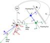 |
Fig. 1 Geometrical properties of the interaction of a planetary body with its
surrounding magnetized plasma with B0: unperturbed stellar
wind magnetic field, vsw: stellar wind velocity,
vorbit: orbital velocity of planet,
v0: relative velocity between planet and stellar wind
plasma, Mexo: magnetic moment of planet (in this figure it
points out of the displayed plane), |

In this work we calculate the energy fluxes radiated away from the obstacles. We assume that in the vicinity of the extrasolar planets (or planetary moons) the incoming stellar wind properties (or magnetospheric plasma properties) can be considered spatially homogeneous on the scales of the local plasma interaction. The energy fluxes generated at the planets (moons) are calculated through a plane which is chosen to be sufficiently far away from the planets (or moons) such that other waves modes than the shear Alfvén modes do not play a role any more. But the location of the plane is still chosen close enough to the planet (or moon) such that the stellar wind properties can still be considered spatially homogeneous and, e.g. the bend of the Parker spiral or the curvature of the magnetospheric fields do not need to be considered. Typical distances of the plane from the planetary obstacles are several times the diameter of the obstacle, whose sizes will be discussed further below.
For the overall stellar wind flow, we assume that the velocity
vsw is strictly radially away from the star. We also assume
without restriction of generality that the magnetic field direction of the stellar wind
points away from the star. The planets move in orbital direction with Kepler velocity
vorbit, which leads to a relative velocity between the planet
and the stellar wind of  (5)One
of the two Alfvén wings generated in the interaction always points away from the star.
With our choice of magnetic field orientations of B0, this is
the
(5)One
of the two Alfvén wings generated in the interaction always points away from the star.
With our choice of magnetic field orientations of B0, this is
the  -wing. We
therefore focus in this study on the
-wing. We
therefore focus in this study on the  -wing (see
Fig. 1). The expressions in the remainder of this
work thus hold for the -wing, but
could similarly be derived for the -wing. In
the remainder of the manuscript we drop for simplicity of notation the superscript
“−” on the quantities describing the
-wing.
-wing (see
Fig. 1). The expressions in the remainder of this
work thus hold for the -wing, but
could similarly be derived for the -wing. In
the remainder of the manuscript we drop for simplicity of notation the superscript
“−” on the quantities describing the
-wing.
For the moon-magnetosphere interaction, the geometry is different. The plasma flow
vp is mostly in the orbital direction of the moon and the
magnetic field is nearly perpendicular to the flow. The relative velocity
v0 thus can be written ![Mathematical equation: \begin{eqnarray} \label{e_v_0_moon} {\vec{v}_0}&=&{\vec{v}_{\rm p}}-{\vec{v}_{\rm orbit}} \nonumber \\[2mm] &\approx& (\Omega r_{\rm s} - v_{\rm orbit}) \; {\vec{\hat{e}}_{\rm orbit}} , \end{eqnarray}](/articles/aa/full_html/2013/04/aa18179-11/aa18179-11-eq42.png) (6)where
Ω is the angular velocity of the central planet,
rs the distance of the satellite from
the planet’s spin axis and êorbit the unit vector in orbital
direction of the satellite (all three quantities as given in an inertial rest frame). In
the moon-planet interaction both wings couple to the planet. In analogy with the
exoplanet-star coupling, we will focus in the moon-planet interaction on the
-wing as
well.
(6)where
Ω is the angular velocity of the central planet,
rs the distance of the satellite from
the planet’s spin axis and êorbit the unit vector in orbital
direction of the satellite (all three quantities as given in an inertial rest frame). In
the moon-planet interaction both wings couple to the planet. In analogy with the
exoplanet-star coupling, we will focus in the moon-planet interaction on the
-wing as
well.
We stress that in the analysis of this paper we use two separate frame of references,
within which we apply two separate coordinate systems. One frame of reference is the
rest frame of the obstacle which launches the Alfvén waves. In the rest frame of the
obstacle the Alfvén wings are steady state under the assumption that the upstream
conditions and the properties of the obstacle are steady state. The other frame of
reference is rotating with the central body, i.e. the star or the central planet, at the
radial distance of the exoplanet or the moon, respectively. In this frame of reference
the Alfvén wings are time-dependent as an observer in this rest frame sees the wings
being convected across the observer with time. These two frames of reference are
connected by a transformation with a constant velocity vT, whose
direction and amplitude will be discussed in Sect. 2.1.3. We also use two separate coordinate systems applicable in each frame of
reference (see Fig. 1). One coordinate system is
called Alfvén wing system (Neubauer 1980). The
Alfvén wing coordinate system in the reference frame of the obstacle is defined as
follows: the z-axis is parallel to the Alfvén wing, i.e. parallel to
. The
y-axis is along the
v0 × B0 direction and the
x-axis completes a right-handed coordinate system, i.e. lies in a
plane defined by v0 and B0. The second
coordinate system is called the B0 magnetic field system or
primed system. In the rest frame of the obstacle it is defined as follows: the
z′ axis is anti-parallel to B0,
the y′ axis is in direction of
vorb × B0, and
x′ completes a right-handed coordinate system. The wing
coordinate system (unprimed system) and the magnetic field system (primed system) within
the same frame of reference are related through  The
angle ΘA describes the inclination of the Alfvén wing with respect to the
background magnetic field (for the exact definition see (19)). The Alfvén wing coordinate system and the
B0 magnetic field coordinate system in the rest frame of the
rotating central body have coordinate axes in the same directions as the associated
coordinate systems in the rest frame of the obstacle.
The
angle ΘA describes the inclination of the Alfvén wing with respect to the
background magnetic field (for the exact definition see (19)). The Alfvén wing coordinate system and the
B0 magnetic field coordinate system in the rest frame of the
rotating central body have coordinate axes in the same directions as the associated
coordinate systems in the rest frame of the obstacle.
If | vT| ≪ c with c being
the speed of light, the variables are related by a Galilei transformation between both
frames of references. Denoting the variables in the rest frame of the obstacle with the
superscript obst and variables in the rest frame of the rotating
central body without any extra superscript, the plasma velocities in both frames are
related by  (10)the
electric fields by
(10)the
electric fields by  (11)and
the magnetic fields by
(11)and
the magnetic fields by  (12)respectively.
2.1.2. Model properties of the Alfvén wings
If the planetary body including its atmosphere is electrically conductive and/or possesses a sufficiently strong internal magnetic field, the plasma flow in the vicinity of the body is slowed and the electric field is reduced. Simple models of the resultant electric field in sub-Alfvénic plasma interaction have been derived by Neubauer (1980, 1998), Saur et al. (1999), or Saur (2004), where the electric currents through the planetary bodies, ionospheres/atmospheres/magnetospheres are closed in the Alfvén waves, which are launched by the interaction.
In these models, the relative strength of the sub-Alfvénic interaction is characterized
by a factor  . This
factor assumes
. This
factor assumes  when
no interaction takes place, i.e. the obstacles do not perturb the plasma flow, and
when
no interaction takes place, i.e. the obstacles do not perturb the plasma flow, and
 for
maximum interaction strength, i.e., the obstacles bring the exterior flow to a complete
halt in its immediate vicinity. The factor is defined by
for
maximum interaction strength, i.e., the obstacles bring the exterior flow to a complete
halt in its immediate vicinity. The factor is defined by
 i.e.,
it is related to how strongly the motional electric field and the plasma velocity in the
vicinity of the obstacle is reduced due to the interaction.
i.e.,
it is related to how strongly the motional electric field and the plasma velocity in the
vicinity of the obstacle is reduced due to the interaction.
In the model applied here the effects of the obstacles are simplified such that the
resultant electric currents reduce the electric field Eobst
within the obstacle of radius R to a constant amplitude
 . Writing
the electric field in terms of the electric potential with
Eobst = −∇Φobst leads to
. Writing
the electric field in terms of the electric potential with
Eobst = −∇Φobst leads to  (15)Outside
of the obstacle and perpendicular to z, the perturbation electric field
decays as a two-dimensional dipole field
(15)Outside
of the obstacle and perpendicular to z, the perturbation electric field
decays as a two-dimensional dipole field  (16)This
electric potential and the resultant electric field map into the Alfvén wings where they
exhibit a two-dimensional structure with translational invariance along the wings
similar to the other plasma properties in the wings (Neubauer 1980). In expressions (15) and (16), we use the
radial distance r of spherical coordinates with
x = rcosϕ and
y = rsinϕ. The radius of the
obstacle R is in case of a nonmagnetized obstacle the radius of the
planet including its atmosphere/ionosphere. In case of a magnetized body, the effective
radius Reff depends on the properties of the internal and
external magnetic field as detailed in Sect. 2.3.
(16)This
electric potential and the resultant electric field map into the Alfvén wings where they
exhibit a two-dimensional structure with translational invariance along the wings
similar to the other plasma properties in the wings (Neubauer 1980). In expressions (15) and (16), we use the
radial distance r of spherical coordinates with
x = rcosϕ and
y = rsinϕ. The radius of the
obstacle R is in case of a nonmagnetized obstacle the radius of the
planet including its atmosphere/ionosphere. In case of a magnetized body, the effective
radius Reff depends on the properties of the internal and
external magnetic field as detailed in Sect. 2.3.
In case of the obstacle being created by an ionosphere whose conductance is given by
the Pedersen conductance ΣP within R, then the interaction
strength can be
approximated (Neubauer 1998; Saur et al. 1999) by  (17)The
Pedersen conductance ΣP is calculated by integrating the local Pedersen
conductivity σp along the magnetic field lines through the
planet’s ionosphere beginning at the magnetic equator (e.g., Neubauer 1998; Saur et al.
1999). The Pedersen conductance is here assumed to be spatially constant within
the ionosphere. In (17), we neglect the
Hall conductance since the Hall currents are perpendicular to the electric field and
thus only indirectly contribute to the energy budget of the interaction by modifying the
overall electric and flow field. Note, also other physical reasons can slow and modify
the flow near the obstacle. Examples are intrinsic magnetic fields (e.g., Ganymede see
Kivelson et al. 1996a) or the effects of a
plasma absorbing body such as Rhea, see Simon et al.
2012).
(17)The
Pedersen conductance ΣP is calculated by integrating the local Pedersen
conductivity σp along the magnetic field lines through the
planet’s ionosphere beginning at the magnetic equator (e.g., Neubauer 1998; Saur et al.
1999). The Pedersen conductance is here assumed to be spatially constant within
the ionosphere. In (17), we neglect the
Hall conductance since the Hall currents are perpendicular to the electric field and
thus only indirectly contribute to the energy budget of the interaction by modifying the
overall electric and flow field. Note, also other physical reasons can slow and modify
the flow near the obstacle. Examples are intrinsic magnetic fields (e.g., Ganymede see
Kivelson et al. 1996a) or the effects of a
plasma absorbing body such as Rhea, see Simon et al.
2012).
The Alfvén conductance ΣA in (17) controls the maximum current which can be carried by an Alfvén wave. It is
given after Neubauer (1980) by  (18)The
Alfvén wing is inclined with respect to the local background magnetic field
(18)The
Alfvén wing is inclined with respect to the local background magnetic field
 by the
angle ΘA (see Fig. 1), which reads
by the
angle ΘA (see Fig. 1), which reads
 (19)The
constancy of the Elsasser variables and a given electric field (e.g. with Eqs. (15) and (16)), constrains the magnetic field in an Alfvén wing after Neubauer (1980) to
(19)The
constancy of the Elsasser variables and a given electric field (e.g. with Eqs. (15) and (16)), constrains the magnetic field in an Alfvén wing after Neubauer (1980) to 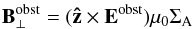 (20)where
⊥ denotes here the direction perpendicular to the wing, ẑ is the unit
vector in the z-direction and
(20)where
⊥ denotes here the direction perpendicular to the wing, ẑ is the unit
vector in the z-direction and  (21)
(21)
2.1.3. Model energy fluxes in Alfvén wing
The Poynting flux, the kinetic and the thermal energy fluxes depend on the frame of
reference. Even though the Alfvén wing is steady state in the rest frame of the obstacle
for steady state upstream and planetary conditions, we are interested in the energy
fluxes deposited into the central bodies. For the calculations of the energy fluxes, we
therefore describe the plasma in a frame of reference moving with the central body (the
star or the central planet) at a radial distance of the obstacle. We choose to calculate
the fluxes at the radial distance of the obstacle because we are interested to determine
the fluxes that are generated locally by the obstacle. With that choice there is no
relative motion of the reference frame toward or away from the central body and the
analysis plane through, which we calculate the energy fluxes does not move with respect
to the central body. Note that a reference frame which would fully move with the plasma
would generally not meet this criteria. The transformation from the rest frame of the
obstacle to the rotating frame of the central body is given by
 where
Ω is the angular velocity of the central body, robst the
distance between the central body and the obstacle, êorbit the
unit vector in orbital direction of the obstacle (all three as seen from an inertial
rest frame).
where
Ω is the angular velocity of the central body, robst the
distance between the central body and the obstacle, êorbit the
unit vector in orbital direction of the obstacle (all three as seen from an inertial
rest frame).
In the Alfvén wing coordinate system, the transformation vT
from the rest frame of the obstacle into the rotating frame of reference is given by the
velocity vector vT:  where
where
 represents the relative velocity between the obstacle and the unperturbed plasma flow.
This transformation is applicable for, both, the extra solar planets with relative
plasma velocities given in (5) and the
satellites at the outer planets with velocities given in (6). The factor γ covers both cases and considers the
different geometrical properties of the interaction at the moons or the extra solar
planets. The factor γ also describes the velocity of the plasma
parallel to the background magnetic field.
represents the relative velocity between the obstacle and the unperturbed plasma flow.
This transformation is applicable for, both, the extra solar planets with relative
plasma velocities given in (5) and the
satellites at the outer planets with velocities given in (6). The factor γ covers both cases and considers the
different geometrical properties of the interaction at the moons or the extra solar
planets. The factor γ also describes the velocity of the plasma
parallel to the background magnetic field.
For the extrasolar planets where the magnetic field is inclined by the Parker angle
θB with respect to the radial direction we find
 (27)With
this choice of γ it can readily be shown that the resultant frame of
reference is a frame that rotates with the angular velocity of the star
Ω⋆ at the radial distance of the extrasolar planet
rexo assuming the Parker model with its frozen-in-field
approximation for the stellar wind. The Parker angle ΘB, i.e. the angle
between the radial direction and the direction of the magnetic field, is given by
(27)With
this choice of γ it can readily be shown that the resultant frame of
reference is a frame that rotates with the angular velocity of the star
Ω⋆ at the radial distance of the extrasolar planet
rexo assuming the Parker model with its frozen-in-field
approximation for the stellar wind. The Parker angle ΘB, i.e. the angle
between the radial direction and the direction of the magnetic field, is given by
 (28)For
the satellites in the outer solar system where the orbital velocities of the moons and
the unperturbed magnetospheric fields are approximately perpendicular, we find
(28)For
the satellites in the outer solar system where the orbital velocities of the moons and
the unperturbed magnetospheric fields are approximately perpendicular, we find
 (29)and
assume cosΘ = 0. With this choice of transformation the new frame of reference is thus a
frame which moves with the angular velocity of the central planet at the radial distance
of the moon.
(29)and
assume cosΘ = 0. With this choice of transformation the new frame of reference is thus a
frame which moves with the angular velocity of the central planet at the radial distance
of the moon.
With the transformation of expressions (24) to (24), the resulting
frame of reference is a frame where the relative velocity
v0, ⊥ perpendicular to the background
magnetic field B0 vanishes, i.e. a frame of reference which
“moves with the magnetic field”. In the rotating frame of reference, the Alfvén wave
travels parallel or anti-parallel to the unperturbed magnetic field and thus the group
velocity of the Alfvén wave is parallel or anti-parallel to B0
(see Eq. (4)). The velocity component
v0, ∥ parallel to the background magnetic
field is approximately zero in the case of the moon planet interaction. However, the
velocity component v0, ∥ parallel to the
background magnetic field is non zero in the case of the extra solar planets and assumes
a value of  .
.
In the rotating frame of reference shifted by vT the
unperturbed motional electric field  vanishes and the net electric field E is given by expression (11). Note, however, that the velocity
component parallel
to B0 makes a nonnegligible contribution in (11) because the cross product of
vT is taken with the perturbed magnetic field
B(x) and not with B0.
vanishes and the net electric field E is given by expression (11). Note, however, that the velocity
component parallel
to B0 makes a nonnegligible contribution in (11) because the cross product of
vT is taken with the perturbed magnetic field
B(x) and not with B0.
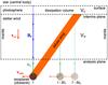 |
Fig. 2 Sketch of the Alfvén wing and its associated dissipation region for idealized stellar wind properties in a frame of reference rotating with the central body. The idealized orientations of the vector fields in the sketch resemble the situation when the radius of the star R⋆ is much larger than the effective radius of the extra solar planet Reff and the angular velocity of the star, the radial distance of the extra solar planet and the stellar wind velocity obey Ω⋆rexo/vsw ≪ 1. The sketch displays the wing at time t and also indicates the time-variability of the wing in the rotating frame. At time t the extra solar planet is situated at a location marked with a brown circle. The extra solar planet in this frame of reference was located at earlier times t − Δt further to the right. The extra solar planet steadily launches Alfvén waves, which travel parallel to B0. The superposition of the wave packets launched at earlier times results in the snapshot of the wing at time t displayed here. |
The time-constant, standing Alfvén wing in the obstacle frame of reference is a
structure moving with vT and is thus time-variable in the
rotating frame of reference. In the rotating frame, the group velocity of the Alfvén
waves and the Elsasser variable are
parallel to the background magnetic field B0, but the Alfvén
wing for a given time t is still inclined by the angle ΘA
with respect to B0 (see also Fig. 2).
In the rotating frame of reference and using the Alfvén wing coordinate system, we can
now derive expressions for the Poynting flux S. Because the expressions are
time-dependent in the rotating frame, we have to evaluate the Poynting flux at a certain
time t. We can choose t without loss of generality
such that the center of the wing is located at x′ = 0 and
y′ = 0 for a certain z′. With
(2), (11), (12), (15), (20), and (21) we
find for the Poynting flux within the inner part of the Alfvén wing, i.e. for
r ≤ R The
Poynting flux in the inner part is spatially constant due to the model assumptions,
which enter into expression (15). With
(2), (11), (12), (16), (20), and (21), we
find for the Poynting flux in the exterior part of the Alfvén wing, i.e. for
r > R,
The
Poynting flux in the inner part is spatially constant due to the model assumptions,
which enter into expression (15). With
(2), (11), (12), (16), (20), and (21), we
find for the Poynting flux in the exterior part of the Alfvén wing, i.e. for
r > R, ![Mathematical equation: \begin{eqnarray} S_{\rm x}^{\rm e}/S_0 &= & -4 \alphabar^2 R^4 x^2 y^2 \sin^2 \Theta_{\rm A} \Gamma_4/r^8 \nonumber \\ && -\,\Gamma_2 [-\Gamma_3 + \Gamma_3 \sin\Theta_{\rm A} (-\gamma \cos\Theta_{\rm A}/\!\cos \Theta+\sin\Theta_{\rm A})\nonumber \\ \label{e_S_x_e} && +\, \Gamma_4 \Gamma_2] \\ \label{e_S_y_e} S_{\rm y}^{\rm e}/S_0 &= & - 2 \alphabar R^2 x y (\Gamma_3 \sin^2 \Theta_{\rm A} + \Gamma_2 \cos \Theta_{\rm A}) \Gamma_4 /r^4 \\ S_{\rm z}^{\rm e}/S_0 &= & \sin \Theta_{\rm A} \left\{ 4 \alphabar^2 R^4 x^2 y^2 \cos \Theta_{\rm A} \Gamma_4 /r^8 \right. \nonumber \\ \label{e_S_z_e} && -\Gamma_3 [-\Gamma_3 + \Gamma_3 \sin\Theta_{\rm A} (-\gamma \cos\Theta_{\rm A} / \!\cos \Theta+\sin\Theta_{\rm A})\nonumber \\ &&+\Gamma_4 \Gamma_2] \left. \right\} \end{eqnarray}](/articles/aa/full_html/2013/04/aa18179-11/aa18179-11-eq117.png) with
the abbreviations
with
the abbreviations 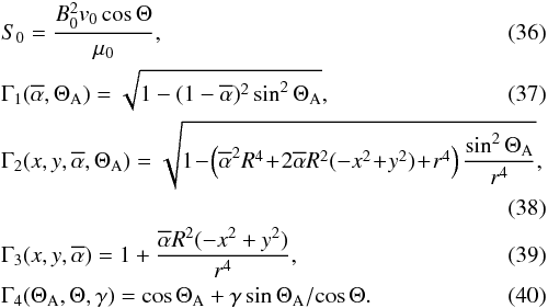 In
the Alfvén wings, also kinetic and thermal energy are convected away from the obstacle.
Constancy of the Elsasser variable or Alfvén characteristic (see Eq. (4)) can be used to calculate the plasma
velocity
In
the Alfvén wings, also kinetic and thermal energy are convected away from the obstacle.
Constancy of the Elsasser variable or Alfvén characteristic (see Eq. (4)) can be used to calculate the plasma
velocity 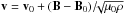 in the
  Alfvén
wing. Using the same frame of reference and coordinate system as for the calculation of
the Poynting flux, we find for the velocity field in the inner part of the wing (i.e.,
r < R)
Alfvén
wing. Using the same frame of reference and coordinate system as for the calculation of
the Poynting flux, we find for the velocity field in the inner part of the wing (i.e.,
r < R) 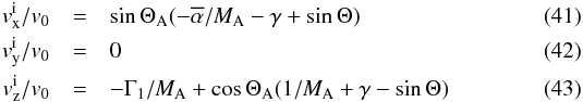 and
in the exterior part (i.e.
r > R)
and
in the exterior part (i.e.
r > R) 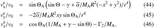 This
velocity field v determines the resultant kinetic energy flux
Fk = 1/2ρv2v
and enthalpy flux
FT = 5/2kB2ρ/mTv,
where T is the plasma temperature, kB the
Boltzmann constant and m the average ion mass of the flow. The factor
of 2 enters if we assume that the ions and electrons have equal temperature. It provides
additional contributions by the wing to the Joule dissipation in Eq. (1) in the rotating frame.
This
velocity field v determines the resultant kinetic energy flux
Fk = 1/2ρv2v
and enthalpy flux
FT = 5/2kB2ρ/mTv,
where T is the plasma temperature, kB the
Boltzmann constant and m the average ion mass of the flow. The factor
of 2 enters if we assume that the ions and electrons have equal temperature. It provides
additional contributions by the wing to the Joule dissipation in Eq. (1) in the rotating frame.
2.1.4. Total energy fluxes toward the central body
In this work we are interested in the energy sources
QD responsible for generating X-ray,
UV, optical and IR emissions at the central body due to the sub-Alfvénic interaction
with an obstacle. A likely candidate for this energy source is Joule dissipation of
electromagnetic field energy feed by the Poynting flux. For further clarifications on
how to determine the total Poynting flux communicated by the interaction toward the
central body, it is helpful to return to Poynting’s theorem (1). In MHD the electric field energy can be
neglected compared to magnetic field energy as their ratio is proportional to
(v/c)2. The time
derivates of the magnetic field energy also vanishes because | B | is
constant within the Alfvén wing under the assumptions discussed in Sect. 2.1.2. We integrate (1) over a volume V which starts “above” the obstacle
but it includes the Alfvén wing and the part of the central body where the
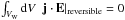
electromagnetic field energy is dissipated (see Fig. 2 for a simplified geometry). The resultant equation reads 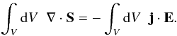 (47)Within
a volume VW, which includes the Alfvén wing
and which is outside of the obstacle and the central body, the term
j·E describes the reversible work done by the
electromagnetic field on the plasma and vice versa, i.e. the acceleration and
deceleration of the flow. Within a volume VD which includes
the close proximity of the central body, we assume that j·E
describes the irreversible, dissipative work done by the electromagnetic field. The
Volume
V = VW + VD
has a surface consisting of three parts: (1) a mantle; (2) an upper lit (or surface)
which is located between the dissipation volume VD and the
interior of the central body and (3) a lower lit (or analysis plane) where the Alfvén
wave generated by the interaction at the obstacle enters the volume. Applying Gauss
Theorem, (47) reads
(47)Within
a volume VW, which includes the Alfvén wing
and which is outside of the obstacle and the central body, the term
j·E describes the reversible work done by the
electromagnetic field on the plasma and vice versa, i.e. the acceleration and
deceleration of the flow. Within a volume VD which includes
the close proximity of the central body, we assume that j·E
describes the irreversible, dissipative work done by the electromagnetic field. The
Volume
V = VW + VD
has a surface consisting of three parts: (1) a mantle; (2) an upper lit (or surface)
which is located between the dissipation volume VD and the
interior of the central body and (3) a lower lit (or analysis plane) where the Alfvén
wave generated by the interaction at the obstacle enters the volume. Applying Gauss
Theorem, (47) reads
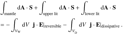 (48)The
surface integral of the Poynting flux through the mantle disappears when the mantle is
displaced sufficiently far away from the wing because the Poynting flux in (33 ) to (35) decreases with r-2 for large
r if r characterizes the distance from the wing
center to the mantle. Because the mantle area grows proportional to the product of
r H, where H is the length of the
wing, the Poynting flux through the mantle decrease to zero with r
growing infinitely. The Poynting flux through the upper lit is zero because we assume
that the flux is being absorbed in the dissipation volume
VD. Thus only the Poynting flux through the lower lit is non
zero. In this analysis we are not interested to measure the conversion of
electromagnetic energy to mechanical energy, thus we need to choose the volume
VW such that the integral over
j·E|reversible vanishes. Under this assumption
(48) simplifies to
(48)The
surface integral of the Poynting flux through the mantle disappears when the mantle is
displaced sufficiently far away from the wing because the Poynting flux in (33 ) to (35) decreases with r-2 for large
r if r characterizes the distance from the wing
center to the mantle. Because the mantle area grows proportional to the product of
r H, where H is the length of the
wing, the Poynting flux through the mantle decrease to zero with r
growing infinitely. The Poynting flux through the upper lit is zero because we assume
that the flux is being absorbed in the dissipation volume
VD. Thus only the Poynting flux through the lower lit is non
zero. In this analysis we are not interested to measure the conversion of
electromagnetic energy to mechanical energy, thus we need to choose the volume
VW such that the integral over
j·E|reversible vanishes. Under this assumption
(48) simplifies to 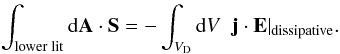 (49)The
integral on the right hand side of (49)
represents the dissipated electromagnetic field energy and will be abbreviated by
QD. In (49) the surface integral on the left hand side describes the Poynting flux in
direction of the outer normal to the lower lit of the volume
VW. Because the obstacle generates an energy flux into the
volume anti-parallel to the outer normal, we convert the sign in this integral and and
call the ingoing flux through the lower lit: the Poynting flux through the analysis
plane. Thus we can write
(49)The
integral on the right hand side of (49)
represents the dissipated electromagnetic field energy and will be abbreviated by
QD. In (49) the surface integral on the left hand side describes the Poynting flux in
direction of the outer normal to the lower lit of the volume
VW. Because the obstacle generates an energy flux into the
volume anti-parallel to the outer normal, we convert the sign in this integral and and
call the ingoing flux through the lower lit: the Poynting flux through the analysis
plane. Thus we can write 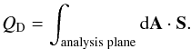 (50)The
orientation of the analysis plane needs to be chosen such that
(50)The
orientation of the analysis plane needs to be chosen such that
 . The
upper lit of the volume is assumed to be approximately parallel to the surface of the
central body. We assume the magnetic field near the central body to be approximately
perpendicular to the surface. In order for the volume integral over
j·E|reversible to disappear the analysis plane
also needs to be perpendicular to the magnetic field B0. This
choice of the analysis plane is consistent with the group velocity of the Alfvén wave
toward the central body being anti-parallel to B0 in the
rotating rest frame, in which this analysis is performed. In the wing directed toward
the central body, the wave travels parallel to
. The
upper lit of the volume is assumed to be approximately parallel to the surface of the
central body. We assume the magnetic field near the central body to be approximately
perpendicular to the surface. In order for the volume integral over
j·E|reversible to disappear the analysis plane
also needs to be perpendicular to the magnetic field B0. This
choice of the analysis plane is consistent with the group velocity of the Alfvén wave
toward the central body being anti-parallel to B0 in the
rotating rest frame, in which this analysis is performed. In the wing directed toward
the central body, the wave travels parallel to
 (51)To
calculate the fluxes through the analysis plane, we therefore multiply the Poynting
fluxes and the respective velocity field components in Eqs. (30) to (35) and (41) to
(46) with
êz′.
(51)To
calculate the fluxes through the analysis plane, we therefore multiply the Poynting
fluxes and the respective velocity field components in Eqs. (30) to (35) and (41) to
(46) with
êz′.
The choice of the analysis plane perpendicular to the background magnetic field B0 as motivated in the previous paragraphs implies interesting consequences for the resulting Poynting flux. The Poynting flux through this analysis decreases with r′-4 for large distances from the wing center. The total, i.e. spatially integrated, Poynting flux therefore stays finite. The Poynting flux through any other analysis plane decreases with r′-2 for large distances from the wing center. The total Poynting flux in certain segments of these other planes therefore can assume infinite values.
To display the Poynting flux through the analysis plane, it is convenient to apply the
primed coordinate system where x′ and
y′ are perpendicular to B0. The
primed Cartesian coordinates can also be expressed in spherical coordinates through
x′ = r′cosϕ′
and
y′ = r′sinϕ′.
The Alfvén wing cuts through the plane perpendicular to B0
inclined by the angle ΘA and thus a circle with radius R
turns into an ellipse given by
x′2cos2ΘA + y′2 = R2
or equivalently described by 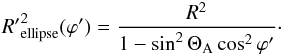 (52)The
total flux Stotal is given by the integral of the Poynting
flux
(52)The
total flux Stotal is given by the integral of the Poynting
flux  and
and
 over the
plane perpendicular to B0
over the
plane perpendicular to B0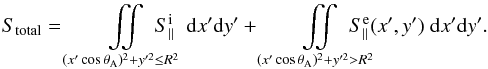 (53)If
the Alfvén Mach number
MA = v0/vA
assumes small values, i.e. in the limit MA → 0, the total
Poynting flux toward the star resulting from expression (53) can be strongly simplified to
(53)If
the Alfvén Mach number
MA = v0/vA
assumes small values, i.e. in the limit MA → 0, the total
Poynting flux toward the star resulting from expression (53) can be strongly simplified to 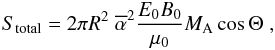 (54)which
also can be rewritten as
(54)which
also can be rewritten as 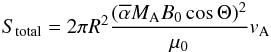 (55)i.e.,
the total flux is for small MA proportional to the square of
the magnetic field perturbation
(55)i.e.,
the total flux is for small MA proportional to the square of
the magnetic field perturbation  generated by the interaction
times the Alfvén velocity vA by which the energy is radiated
away. As will be discussed in Sect. 2.2, the
simplified expressions for the total Poynting flux in (54) or (55) might be
useful approximations in a series of cases. These expressions differ from the
expressions in Zarka (2007) and Lanza (2009) next to other details by a factor of
2v/vA. We note that
the energy dissipation in the central body and in the obstacle are not symmetric. The
energy dissipation in the obstacles’s ionosphere renders a maximum for interaction
strength
generated by the interaction
times the Alfvén velocity vA by which the energy is radiated
away. As will be discussed in Sect. 2.2, the
simplified expressions for the total Poynting flux in (54) or (55) might be
useful approximations in a series of cases. These expressions differ from the
expressions in Zarka (2007) and Lanza (2009) next to other details by a factor of
2v/vA. We note that
the energy dissipation in the central body and in the obstacle are not symmetric. The
energy dissipation in the obstacles’s ionosphere renders a maximum for interaction
strength  (Neubauer 1980), while the Poynting flux in
expression (55) maximizes for maximum
interaction strength .
(Neubauer 1980), while the Poynting flux in
expression (55) maximizes for maximum
interaction strength .
The kinetic and thermal energy fluxes are calculated similarly through a plane
perpendicular to B0. In our rest frame, the background velocity
v0, i.e. the velocity sufficiently far away from the obstacle
is purely parallel to B0 and thus also anti-parallel to the
group velocity of the Alfvén wave. For extra solar planets v0
points away from the central star. We are interested in the total energy fluxes toward
the central star and thus integrate the kinetic and thermal energy fluxes where the
velocity vector parallel to B0 points toward the star, i.e.
where  .
.
2.2. Properties of the Poynting flux within the Alfvén wing
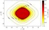 |
Fig. 3 Poynting flux through a plane perpendicular to B0 for
Alfvén Mach number MA = 0.8, interaction strength
|
We display the Poynting flux
S∥ = S·êz′
in Fig. 3 for an Alfvén Mach number
MA = 0.8, an interaction strength
 and
Θ = 0, i.e the magnetic field and plasma flow are perpendicular to each other. The
Poynting flux is positive everywhere, i.e. points away from the obstacle toward the
central body. In our model, the Poynting flux is constant
in the inner part of the Alfvén wing, i.e. within the ellipse given by
r′ < R′ellipse
(see Eq. (52)). The Poynting flux achieves
its maximum values on the flanks of the wing, i.e. near x′ = 0
and | y′| > R. The
Poynting flux decreases as r-4 at larger distance from the
wing.
and
Θ = 0, i.e the magnetic field and plasma flow are perpendicular to each other. The
Poynting flux is positive everywhere, i.e. points away from the obstacle toward the
central body. In our model, the Poynting flux is constant
in the inner part of the Alfvén wing, i.e. within the ellipse given by
r′ < R′ellipse
(see Eq. (52)). The Poynting flux achieves
its maximum values on the flanks of the wing, i.e. near x′ = 0
and | y′| > R. The
Poynting flux decreases as r-4 at larger distance from the
wing.
In Fig. 4 we show the total Poynting flux calculated
with expression (53) as a function of the
interaction strength for
MA = 0.04, MA = 0.4 and
MA = 0.66 as solid lines. We also show for comparison the
simple approximation of the Poynting flux given by the expressions in (54) or (55) as dashed lines. For small MA the
approximation fits the full expression very well, but even for large
MA both the full and simplified expression are still in
reasonable agreement. Therefore the simple and “user friendly” expressions for the total
Poynting flux provided in (54) or (55) might be used in a series of applications.
 |
Fig. 4 Total Poynting flux through a plane perpendicular to B0 as
a function of the interaction strength |
For large Alfvén Mach numbers MA, which obey the condition
 (56)the
argument of the root in (35) turns
negative for selected locations of x and y. In the case
where the incident plasma flow is perpendicular to the background magnetic field, i.e.
Θ = 0, the condition simplifies to
(56)the
argument of the root in (35) turns
negative for selected locations of x and y. In the case
where the incident plasma flow is perpendicular to the background magnetic field, i.e.
Θ = 0, the condition simplifies to  .
Assuming additionally , the
condition reads
.
Assuming additionally , the
condition reads  or ΘA > 30°. For the parameter space where
(56) is fulfilled, the expression in
(35) cannot be used to calculate the
Poynting flux. This effect is visible in Fig. 4 for
the upper curves with MA = 0.66. Under this circumstance the
upper solid line only extends to
or ΘA > 30°. For the parameter space where
(56) is fulfilled, the expression in
(35) cannot be used to calculate the
Poynting flux. This effect is visible in Fig. 4 for
the upper curves with MA = 0.66. Under this circumstance the
upper solid line only extends to  . In case condition (56) applies in some of the sub-Alfvénic cases
to be discussed in this work, a lower limit can be chosen by using a decreased interaction
strength such that
. In case condition (56) applies in some of the sub-Alfvénic cases
to be discussed in this work, a lower limit can be chosen by using a decreased interaction
strength such that
 .
.
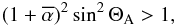
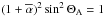
The total Poynting flux also depends on the angle between the incident flow and the
background magnetic field characterized by Θ, which is defined such that Θ = 0, when
B0 and v0 are perpendicular, see Fig.
1. In Fig. 5
we show the total Poynting flux as a function of the incident angle Θ for the Alfvén Mach
numbers MA = 0.04, MA = 0.4,
MA = 0.66 and interaction strength
 . The
total Poynting flux is zero, when the flow is parallel or anti-parallel to the background
magnetic field since the motional electric field in the rest frame of the plasma vanishes.
In reality the obstacle will in this case still generate some perturbations, which are,
however, very small compared to the case when B0 and
v0 are approximately perpendicular. Within the planetary bodies
under consideration in this work, Θ ranges from 0° to 180°. However,
the Poynting flux as a function of Θ is symmetric with respect to Θ = 90°, i.e.
Stotal(90° + Θ) = Stotal(90°−Θ).
In Fig. 5 we therefore display the range
0° ≤ Θ ≤ 90° only, but add for completeness the range
− 90° ≤ Θ ≤ 0°. The Alfvén wing angle ΘA is asymmetric
with respect to the flow angle Θ = 0. The physical reason is that the plasma flow
v0 has contribution parallel to B0 for
Θ ≠ 0. If the flow is parallel to the Alfvén wave vA the tilt of
the Alfvén wing is decreased, i.e. the wing is more aligned with
B0. Figure 5 also shows
that the approximated expression of (55)
shown as dashed lines is for angles Θ ≠ 0 not under all circumstances an upper limit to
the full expression (53) of the total
Poynting flux shown as solid lines.
. The
total Poynting flux is zero, when the flow is parallel or anti-parallel to the background
magnetic field since the motional electric field in the rest frame of the plasma vanishes.
In reality the obstacle will in this case still generate some perturbations, which are,
however, very small compared to the case when B0 and
v0 are approximately perpendicular. Within the planetary bodies
under consideration in this work, Θ ranges from 0° to 180°. However,
the Poynting flux as a function of Θ is symmetric with respect to Θ = 90°, i.e.
Stotal(90° + Θ) = Stotal(90°−Θ).
In Fig. 5 we therefore display the range
0° ≤ Θ ≤ 90° only, but add for completeness the range
− 90° ≤ Θ ≤ 0°. The Alfvén wing angle ΘA is asymmetric
with respect to the flow angle Θ = 0. The physical reason is that the plasma flow
v0 has contribution parallel to B0 for
Θ ≠ 0. If the flow is parallel to the Alfvén wave vA the tilt of
the Alfvén wing is decreased, i.e. the wing is more aligned with
B0. Figure 5 also shows
that the approximated expression of (55)
shown as dashed lines is for angles Θ ≠ 0 not under all circumstances an upper limit to
the full expression (53) of the total
Poynting flux shown as solid lines.
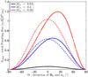 |
Fig. 5 Total Poynting flux as a function of the angle Θ between the background magnetic
field B0 and the incident plasma velocity
v0. The angle Θ is zero, when B0
and v0 are perpendicular (see Fig. 1). The Poynting flux is symmetric with respect to 90°.
For the planetary bodies under consideration in this work, Θ falls into the range
0 ≤ Θ ≤ 180°. Note that in this figure, we additionally show the range
− 90° ≤ Θ ≤ 0° for cases where such an orientation of the
magnetic field and the velocity occur. The interaction strength and the Alfvén Mach
number are chosen as |
2.3. Orientation of planetary magnetic field and effective radius of the obstacle
In case the planetary body possesses an intrinsic magnetic field, the magnetic field environment near the planetary body and thus also the Poynting flux generated by the interaction with the surrounding flow is additionally modified. Here we assume that the internal magnetic field can be characterized by a dipole moment Mexo with equatorial field strength Bexo on the surface of the planetary body. Next to the magnitude of the planetary magnetic field, its orientation with respect to the exterior field B0 plays a crucial role for the total Poynting flux. In Fig. 6 we show the magnetic field environment near the planet where we assume a planetary surface field Bexo of 5000 nT with an associated dipole moment which is inclined by 45° with respect to the stellar wind field B0 of 100 nT. The magnetic field environment can be topologically divided into three areas. I: field lines which start on the planet and end on the planet, II: field lines which start on the planet and end on the star, and III: field lines which never intersect with the planet. The effective width of all field lines belonging to region I, when B0 and the magnetic dipole moment of the extrasolar planet Mexo are parallel is given by
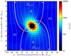 |
Fig. 6 Magnetic field topology and effective radius of Alfvén wings for oblique intrinsic and exterior field orientations. White dotted lines show magnetic field lines and black arrows indicate the magnetic field direction. The field strength is displayed color coded. The boundary, which separates closed field lines starting and ending on the planet from field lines connecting to the star, are displayed as solid white line. The distance of these field lines at larger distance from the planet establishes the effective diameter Deff of the Alfvén wings. |
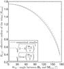 |
Fig. 7 Effective radius of Alfvén wing in units of Robst (see (57)) as a function of the orientation of the intrinsic to the external magnetic field (solid line). Two analytical approximations are shown as dashed and dotted lines. |
 (57)
(57)
Total Poynting fluxes and properties at satellites for average magnetospheric values.
where Rexo is the radius of the extrasolar planet. This
expression is often used to characterize the size of the planetary obstacle in the stellar
wind (e.g. Lanza 2009). However, all field lines
anchored in the planetary ionosphere from class II are slowed depending on the conductance
of the planet’s ionosphere, and thus establish the effective radius of the planet’s
magnetosphere
Reff = 1/2Deff
as displayed in Fig. 6. The effective diameter
Deff is the average distance at which field lines in regions
II are separated at large distance from the planet. The effective radius as a function of
the angle ΘM between the planetary magnetic moment
Mexo and the stellar wind magnetic field
B0 is shown in Fig. 7. For
arbitrary angle ΘM, the values of
Reff need to be calculated numerically (solid line in Fig.
7). When the dipole moment and the stellar magnetic
field are parallel, the effective radius is maximum and a factor of
 larger than Robst. Thus the effective area of the obstacle is
a factor of 3 larger than the area determined by the closed field lines quantified by
Robst in (57) and its assumptions. When the magnetic moment and the stellar wind magnetic
field are anti-parallel, i.e. the planetary field at the magnetic equator and the stellar
wind magnetic field are parallel, the magnetosphere is closed. This effect has been noted
by Ip et al. (2004) and Kopp et al. (2011), but not investigated quantitatively. For
convenience we provide in Fig. 7 two expressions
which approximate the numerical values. Thus the relative orientation of the planetary
magnetic moment and the stellar wind magnetic field has strong effects on the magnitude of
the resulting Poynting flux launched at the planet.
larger than Robst. Thus the effective area of the obstacle is
a factor of 3 larger than the area determined by the closed field lines quantified by
Robst in (57) and its assumptions. When the magnetic moment and the stellar wind magnetic
field are anti-parallel, i.e. the planetary field at the magnetic equator and the stellar
wind magnetic field are parallel, the magnetosphere is closed. This effect has been noted
by Ip et al. (2004) and Kopp et al. (2011), but not investigated quantitatively. For
convenience we provide in Fig. 7 two expressions
which approximate the numerical values. Thus the relative orientation of the planetary
magnetic moment and the stellar wind magnetic field has strong effects on the magnitude of
the resulting Poynting flux launched at the planet.
3. Poynting fluxes generated by the satellites of Jupiter and Saturn
In our solar system, sub-Alfvénic plasma interactions are observed at a number of satellites in the outer solar system (see Sect. 1). We therefore can use these observational constraints to benchmark our derived expressions of the previous section and predict luminosities of possible satellite footprints which have not yet been observed.
3.1. Jupiter’s Galilean satellites
At the Galilean satellites of Jupiter, the Poynting fluxes generated by the interactions are time-dependent and depend on the satellites’ positions in Jupiter’s magnetosphere because Jupiter’s magnetic moment is inclined by ~10° with respect to its spin axis (e.g. Kivelson et al. 2004). Therefore magnetic field strengths, plasma densities and interaction strengths vary with the satellites’ positions in Jupiter’s rotating magnetosphere conveniently measured in system III longitude.
While most quantities in the expressions for the Poynting fluxes (30) and (35) have been measured by spacecraft and are listed in Table 1, the relative strength of the plasma interaction
is not a
directly observable quantity, but can be estimated with the Pedersen conductance of the
satellites’ ionospheres ΣP and the Alfvén conductance ΣA through
(17). The latter two quantities are not
directly measurable either, but the Alfvén conductance ΣA is given by (18) and depends dominantly on the
observationally constrained plasma densities and magnetic field strengths. The Pedersen
conductance ΣP is the local Pedersen conductivity integrated along the magnetic
field lines through the satellites’ ionospheres. The Pedersen conductances have been
modeled in various studies (e.g. Saur et al. 1999,
2002; Kivelson et
al. 2004). For Jupiter’s satellites we use the maximum, spatially averaged
ionospheric conductances ΣP,c listed in Kivelson et al. (2004) as the values in the center of Jupiter’s plasma
sheet. Because the Pedersen conductivity is proportional to the plasma density in the
ionosphere, we scale the variation of the Pedersen conductance ΣP relative to
its values in the center of the Jovian plasma sheet nc with
 (58)When
the torus plasma enters the satellites’ ionospheres unmodified, κ = 1. An
enhanced plasma density through enhanced electron impact ionization can be considered by
κ > 1.
(58)When
the torus plasma enters the satellites’ ionospheres unmodified, κ = 1. An
enhanced plasma density through enhanced electron impact ionization can be considered by
κ > 1.
Due to uncertainties in the detailed spatial variations of the plasma density in Jupiter’s magnetosphere at the locations of the Galilean satellites as a function of system III longitude, we apply in the following Sects. 3.1.1 to 3.1.4 two different models of the plasma densities for each satellite. One set of models is individually constructed based on various sources in the literature and the other model is after Bagenal & Delamere (2011), who provide a model for the plasma properties of Jupiter’s magnetosphere. Due to uncertainties in the variability of the interaction strength as a function of system III longitude, we also investigate its effect on the energy fluxes. Therefore we use the density model of Bagenal & Delamere (2011) and vary the interaction strength by choosing κ = 1 and κ = 2 in (58). For each of the Galilean satellites we therefore apply three models, respectively, to study the variability of the footprint brightness and their dependences on the plasma properties in the vicinity of the Galilean satellites.
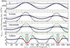 |
Fig. 8 Total Poynting flux generated by the Galilean satellites as a function of system
III longitude for different models of the plasma density and interaction strength.
Solid lines display the Poynting flux with magnetospheric density models after Bagenal & Delamere (2011) calculated with
two different assumptions of the interaction strength
|
3.1.1. Poynting fluxes: Io
The resultant Poynting fluxes at Io as a function of system III are displayed in Fig.
8 in the first panel. The Poynting flux
calculated with the density model extracted in Jacobsen
(2011) based on Bagenal (1994) is shown
as dashed solid line with κ = 2. Additionally, we use the density model
by Bagenal & Delamere (2011) with
κ = 1 and κ = 2 and display the resultant Poynting
fluxes with the thin blue and the thick black line, respectively. The magnetic field
model is based on the composite model including Jupiter’s internal field and the plasma
sheet contributions assembled in Seufert et al.
(2011). For the interaction strength we use (17) and (58) with ΣP,c = 200 S in the center of
the plasma sheet (Saur et al. 1999; Kivelson et al. 2004). We assume an effective radius
due to Io’s ionosphere of
Reff = 1.3 RIo, an average
mass for the torus plasma of 22 amu, and Θ ≈ 0 (Saur et
al. 1999; Kivelson et al. 2004).
Average values for the Poynting flux are on the order of ~1 × 10¹² W. These values can be compared with Hubble Space Telescope (HST) observations. The observed intensities of Io’s footprint in the far-ultraviolet (FUV, i.e. 120–180 nm) typically lie on the order of several 100 kR, where 1 kR = 103 Rayleigh correspond to 1013 photons m-2 s-1 into 4π steradians (Clarke et al. 2002). An emission output in the FUV of 1 kR requires an input energy flux by energetic electrons of ~10-4 W m-2 (e.g., Gérard et al. 2006). In the FUV, an emission of 1 kR corresponds to an energy flux of ~10-5 W m-2. This implies a conversion/efficiency factor of ~10% of the energy input flux by energetic electrons compared to the energy output as FUV photons. If the extreme-ultraviolet spectrum (EUV, i.e. 80–120 nm) is included in addition to the FUV, the conversion factor is ~20% (Gustin et al. 2012; Bonfond et al. 2013). Io’s main footprint displays a brightness in the FUV in the range of 5–700 kR (e.g., Clarke et al. 1996, 1998; Gérard et al. 2006; Wannawichian et al. 2010). The required electron input power to generate these footprint fluxes was derived to lie in the range 4–300 × 109 W (e.g., Prangé et al. 1996; Clarke et al. 1996; Gérard et al. 2006). Very recently, Bonfond et al. (2013) reanalyzed a large set of HST observations of Io’s footprint and found a maximum vertical brightness of approximately ~2–20 × 103 kR in the EUV+FUV with an associated energy input in the range of ~25–200 × 109 W. Our modeled Poynting fluxes lie in the range of 288−1660 × 109 W (see Table 1). Comparison of the observationally derived energy input fluxes with our Poynting fluxes imply that on the order of ~10% of the total Poynting flux of Io’s Alfvén wave/wing is converted into accelerated electrons to generate Io’s main footprint. The rest of the wave energy is (a) partially reflected on its way to Jupiter (Chust et al. 2005; Hess et al. 2010a, 2013), is (b) partially distributed over a larger area including multiple spots and the downstream auroral trail, and is (c) partially converted into other forms of plasma energy, such as heating. But succinctly, the overall energy in the Poynting flux originating at Io is sufficient to generate Io’s auroral footprint.
The quoted brightness of Io’s UV footprints show significant variability. Next to
variations of an apparent random nature, a systematic trend in the total UV intensity is
due to Io’s position with respect to the Jovian plasma sheet with typical values varying
by a factor of ~5 from ~50 kR to ~250 kR according to Wannawichian et al. (2010). Depending on the input torus model used in our
calculations, we see a very weak variability of ~20% (dashed line in upper panel of Fig.
8) up to a variability by a factor of ~5 as a
function of system III longitude (solid lines in upper panel of Fig. 8). The strongest contribution to the variability in
the locally generated Poynting fluxes is due to the variable density with weaker
contributions due to the variable interaction strength
, whereas
the magnetic field strength at Io varies only modestly as a function of system III.
Additional effects of the far-field likely contribute to a stronger variability.
According to Jacobsen et al. (2007), the stronger
the interaction the more nonlinear is the reflection of Io’s Alfvén waves at the
electron acceleration region or Jupiter’s ionosphere characterized by its Pedersen and
Hall conductances. For a fully nonlinear interaction, the Alfvén waves are reflected
back to Io within the original Alfvén waves. In this case no multiple footprints
downstream are seen, but only a downstream tail, as the wave is reflected within itself
(Gérard et al. 2006; Jacobsen et al. 2007). Therefore the wave energy of the multiple
spots is combined, when Io is in the center of the current sheet. Bonfond et al. (2008) report the discovery of a leading spot, i.e. a
precursor spot, when Io is outside the center of the torus. When Io is in the center of
the torus, the leading spot will overlap with Io’s main spot and thus will enhance its
brightness as well. A fraction of the wave energy at Io will be partly reflected and
filamented while traveling along the inhomogeneous plasma densities and magnetic fields
(Wright & Schwartz 1989; Chust et al. 2005; Jacobsen et al. 2007; Hess et al.
2010a, 2011a). The strength of the wave
reflection, transmission and filamentation also depends on Io’s position in the torus
and will contribute to the variably of the brightness (Hess et al. 2013).
3.1.2. Poynting fluxes: Europa
Clarke et al. (2002) report the first observation of an auroral footprint of Europa with brightnesses of a few 10 kR in the FUV. Grodent et al. (2006) measure 14 kR for the main spot, but also observe an auroral tail. Wannawichian et al. (2010) see variations in the FUV spot brightness between 20 and 80 kR. The total emitted power derived by Grodent et al. (2006) is 8 × 10⁸ W with a spot size corresponding to an upper limit of 15 times the diameter of Europa. Clarke et al. (2002) report energy input fluxes for Europa’s footprint of 1−5 × 10⁸ W.
We calculate the total Poynting flux as function of λIII
with the following parameters for three different models: we use
ΣP,c = 30 S which corresponds to
 in
the center of the plasma sheet (Kivelson et al.
2004). We assume an extension of Europa’s interaction region of
Reff = 1.3 REuropa (Saur et al. 1998). The magnetic field is calculated
similar to Io with the model by Seufert et al.
(2011). The dashed curve in Fig. 8 uses
torus electron number densities from Schilling
(2006) with an average ion charge of 1.5 elementary charges and average mass of
18 amu (Kivelson et al. 2004). We extract the ion
density assembled in Schilling (2006) by an
analytic expression of the form
n0 + n1sinγ(λIII − λ0),
with the free parameters n0, n1,
λ0 and γ. For Europa we use for the
electron density n0 = 18 cm-3,
n1 = 232 cm-3,
λ0 = 22.5°, and γ = 4 based on
the values in Schilling (2006) and we use
κ = 2. The solid blue and black lines use the density model of Bagenal & Delamere (2011) with
κ = 1 and κ = 2 , respectively.
in
the center of the plasma sheet (Kivelson et al.
2004). We assume an extension of Europa’s interaction region of
Reff = 1.3 REuropa (Saur et al. 1998). The magnetic field is calculated
similar to Io with the model by Seufert et al.
(2011). The dashed curve in Fig. 8 uses
torus electron number densities from Schilling
(2006) with an average ion charge of 1.5 elementary charges and average mass of
18 amu (Kivelson et al. 2004). We extract the ion
density assembled in Schilling (2006) by an
analytic expression of the form
n0 + n1sinγ(λIII − λ0),
with the free parameters n0, n1,
λ0 and γ. For Europa we use for the
electron density n0 = 18 cm-3,
n1 = 232 cm-3,
λ0 = 22.5°, and γ = 4 based on
the values in Schilling (2006) and we use
κ = 2. The solid blue and black lines use the density model of Bagenal & Delamere (2011) with
κ = 1 and κ = 2 , respectively.
The resulting total Poynting fluxes as function of system III are shown in the second panel of Fig. 8. The total Poynting flux clearly varies as a function of λIII with the maximum values when Europa is in the center of the Jovian plasma sheet. Our model results are consistent with the derived energy input fluxes by HST of 0.1−8 × 10⁹ W (Clarke et al. 2002; Grodent et al. 2006). We find model fluxes in the range of ~0.1–71 × 109 W. These observed values are on the order of ~10% of the total Poynting flux generated at Europa , i.e. similar to Io only a fraction of the total Poynting flux is converted into electron input energies to generate the UV emissions of the central auroral spot. The brightness variability in our model is different for each model. The strongest impact on the variability is due to the variability of the plasma density as a function of system III. The variability of the local interaction strength also contributes to the variability of the Poynting flux and the nonlinearity of the farfield interaction similar to the discussion at Io might play a role as well.
3.1.3. Poynting fluxes: Ganymede
Clarke et al. (2002) first observed the Ganymede footprints in Jupiter’s ionosphere/atmosphere with a brightness of a few 10 kR which requires an energy input of 0.1–0.5 × 10⁹ W. Grodent et al. (2009) derive values for the energy input in the range of 2–15 × 109 W where the auroral footprint matches an area with a diameter of 8–20 RGanymede. Wannawichian et al. (2010) see brightness variations between ~50–150 kR.
We calculate the total Poynting flux as function of λIII
with the following model parameters: we use ΣP,c = 16 S
which is 4 times higher compared to the value referenced in Kivelson et al. (2004), but it leads to more realistic values of the
polar flow velocity in agreement with Jia et al.
(2009). We assume κ = 2. For the torus ion density, we use for
the model displayed as dashed line in Fig. 8 a
similar dependency as for Europa with γ = 4,
n0 = 1 cm-3, n1 = 7
cm-3, and 14 amu as average mass (Kivelson
et al. 2004). This model can be regarded as an upper limit for the variability
as function of system III. The solid blue and the black lines are calculated with
density models from Bagenal & Delamere
(2011) and κ = 1 and κ = 2, respectively. The
magnetic field model is after Seufert et al.
(2011). Ganymede possesses an intrinsic magnetic moment and thus a
mini-magnetosphere within Jupiter’s large magnetosphere (Kivelson et al. 1996a; Neubauer 1998).
The intrinsic magnetic field significantly enlarges the size of the obstacle to the
flow. As discussed in Sect. 2.3 the size of the
open-closed field line area given by (57) is in case when the magnetic moment and the external magnetic field are
parallel enhanced by a factor of .
Thus the effective radius of Ganymede as a source of Alfvén waves is
 , which
assumes values in the range of ≈3.2−3.8 × RGanymede,
depending on Ganymede’s position with respect to the magnetospheric current sheet. Thus
the effective area and the resulting Poynting flux are enhanced by roughly a factor of
10 compared to
, which
assumes values in the range of ≈3.2−3.8 × RGanymede,
depending on Ganymede’s position with respect to the magnetospheric current sheet. Thus
the effective area and the resulting Poynting flux are enhanced by roughly a factor of
10 compared to  due to
Ganymede’s internal magnetic field.
due to
Ganymede’s internal magnetic field.
The total Poynting flux as a function of system III is shown in the third panel of Fig.
8 for our three different models. The total
Poynting flux assumes values as high as ~1.5 × 10¹¹ W with the maximum values
at λIII where Ganymede is in the center of the Jovian plasma
sheet. In the center of the plasma sheet our solution is in the range where it does not
obey the condition (56) any more. In
this case we use the approximate expression for the Poynting flux in (55) as an upper limit (dashed green curve),
and we lower sin(ΘA) in (53)
(to avoid altering ) until
condition (56) is met as a lower limit
(dashed red curve).
The observationally derived energy input fluxes in the range of 0.1−15 × 109 W (Clarke et al. 2002; Grodent et al. 2009) are consistent with our model fluxes which lie in the range of 1−149 × 109 W. Thus also at Ganymede, our predicted Poynting flux is sufficiently large to account for the auroral footprint energy budget. Similarly to Io on the order of ~10% of the generated Poynting flux is converted into electron acceleration to generate Europa’s footprint. Our predicted variability depends strongly on the density model and the model of the interaction strength. Our model variabilities are within the observed variability ranges by Clarke et al. (2002); Grodent et al. (2006); Wannawichian et al. (2010). Also here similar to Io, wave reflection and the nonlinear feedback of the reflected waves might additionally contribute to the variability.
3.1.4. Poynting flux: Callisto
Callisto’s footprints have not yet been fully confirmed observationally. They likely lie within Jupiter’s main auroral oval which has a typical brightness of a few 100 kR. First observational hints for the existence of Callisto’s footprints where presented by Clarke et al. (2011). Here we provide predictions for footprint brightness and variability, as Jupiter’s main auroral oval can shift its location due to variable internal sources and varying solar wind conditions and thus might very occasionally not overlap with a possible footprint of Callisto.
We calculate the total Poynting flux as a function of λIII
for three different models. The dashed black line is calculated with a similar density
dependence as for Europa and Ganymede with minimum and maximum values ranging between
0.001 and 0.5 cm-3 and an average mass of 16 amu (Kivelson et al. 2004) and apply κ = 2 for this
model. The solid blue and the black lines are calculated with density models after Bagenal & Delamere (2011) and
κ = 1 and κ = 2, respectively. We use in the center
of the plasma sheet ΣP,c = 1000 S (Kivelson et al. 2004), which corresponds to an interaction strength
of  (Strobel et al. 2002). The magnetic field model
is after Seufert et al. (2011). The resulting
Poynting fluxes are displayed in the fourth panel of Fig. 8. The total Poynting flux assumes values up to ~5 × 10⁹ W. Near
the center of the plasma sheet (56) is
violated. Thus we calculate similar to the procedure at Ganymede an upper limit (green
dashed curve) and a lower limit (red curve). The grey area indicates cases where the
interaction is super-Alfvénic, i.e.
MA > 1. The theoretical model of
the Alfvén wings by Neubauer (1980) which we
apply has, however, been developed for
MA < 1. All three models predict
that Callisto’s Poynting fluxes are not maximum in the center of the current sheet. The
reason is that at radial distances of Callisto the magnetic field strength in the center
of the current sheet is strongly reduced and even compensates the effects of the
enhanced plasma density within the current sheet.
(Strobel et al. 2002). The magnetic field model
is after Seufert et al. (2011). The resulting
Poynting fluxes are displayed in the fourth panel of Fig. 8. The total Poynting flux assumes values up to ~5 × 10⁹ W. Near
the center of the plasma sheet (56) is
violated. Thus we calculate similar to the procedure at Ganymede an upper limit (green
dashed curve) and a lower limit (red curve). The grey area indicates cases where the
interaction is super-Alfvénic, i.e.
MA > 1. The theoretical model of
the Alfvén wings by Neubauer (1980) which we
apply has, however, been developed for
MA < 1. All three models predict
that Callisto’s Poynting fluxes are not maximum in the center of the current sheet. The
reason is that at radial distances of Callisto the magnetic field strength in the center
of the current sheet is strongly reduced and even compensates the effects of the
enhanced plasma density within the current sheet.
3.1.5. Comparison and comments
Zarka (2007) and Hess et al. (2011a) estimate values for the energies in the interaction of the satellites with Jupiter’s magnetosphere. Our derived values for the Poynting flux are on the same order but somewhat smaller than those in Zarka (2007) since the expressions in Zarka (2007) consider the energy flux into the satellites’ ionospheres or the energies dissipated within the satellites’ ionospheres, which are generally larger than the energy radiated away from the satellites, which we calculate here. Hess et al. (2010b, 2013) also investigate, based on simplified expressions for the local interaction, the variability of the luminosity of the satellites’ footprints focusing on the far-field, i.e. the reflection and filamentation of the waves.
An additional important component which creates variability of the footprint brightness as a function of system III, might be the plasma properties in the region where magnetic field energy is converted into particle acceleration. For Jupiter the auroral acceleration region is thought to occur a few Jovian radii above Jupiter’s ionosphere. In this region the density of ions and energetic electrons might vary with implications on the variability of the footprint brightness as discussed for example in Bonfond et al. (2007); Hess et al. (2011b).
Note that the observationally derived brightnesses and estimated input fluxes for the satellites footprints by the various authors where partially derived under somewhat different assumption and with somewhat different analysis techniques.
Succinctly, the overall energy flux values in the Poynting fluxes originating at the Galilean satellites are sufficient to generate their auroral footprints.
3.2. Poynting flux: Saturn’s inner icy satellites
At Saturn so far only an Enceladus footprint has been observed by Pryor et al. (2011). The observed spot brightness in the UV ranges from 0.45 to 1.55 kR with the size of the spots possibly extending 20 REnceladus downstream. With the values of Table 1, we predict a Poynting flux of ~200 × 106 W. For this value we assumed a maximum interaction strength and a fairly large size of the obstacle. The value thus rather needs to be considered an upper limit. Based on the observed brightness a footprint size corresponding to 1.3 REnceladus with a downstream extension of 20 REnceladus would lead to an auroral electron energy input of ~1−4 × 10⁶ W assuming 1 kR requires an energy input of 1 × 10⁻⁴ W m-2 (Pryor et al. 2011). Thus the predicted Poynting flux is larger and sufficient to account for the UV observations and its large extension. We note that at Enceladus the neutral gas environment possesses a north south asymmetry due the location of the water plume near Enceladus’ south pole (Dougherty et al. 2006; Tokar et al. 2006). This asymmetry in the gas generates asymmetric Alfvén wings and associated asymmetric Poynting fluxes (Saur et al. 2007). Using the asymmetric expressions for the electric fields derived in Saur et al. (2007) or Simon et al. (2011a), these asymmetric fluxes can be calculated in the same manner as in Sect. 2. Due to the electromagnetic coupling of Enceladus’ southern and northern hemispheres (Saur et al. 2007), we expect even in the case where the south polar plume would be located only near and “just below” Enceladus’ south pole, still Poynting flux being radiated into the northern hemisphere of Saturn’s magnetosphere.
Based on the values in Table 1, among the inner icy satellites of Saturn, only Rhea and Dione might produce a Poynting flux which could possibly lead to observable footprints in case of sufficiently long exposure times. Both, Rhea and Dione have sputtering generated atmospheres/exospheres (Saur & Strobel 2005; Teolis et al. 2010; Simon et al. 2011b) which is a root cause for the generation of Alfvén waves. The Poynting fluxes at the satellites of Saturn might vary as a function of time due to varying magnetospheric properties and/or varying neutral atmosphere densities caused by a time variable radiation belt (Roussos et al. 2008; Simon et al. 2011b). Note that Simon et al. (2012) show that the dominant part of the magnetic field perturbations observed by the Cassini spacecraft near Rhea is due to plasma absorption effect caused by the solid body of Rhea. But independent of the root cause of the magnetic field and velocity perturbations near planetary bodies, their resultant Alfvén wings carry Poynting flux toward the central body.
4. Poynting fluxes at extrasolar planets
In this study we investigate the plasma environment at 850 extrasolar planets1 (Schneider et al. 2011). They provide a good statistical ensemble to investigate the possible electromagnetic star-planet coupling at extrasolar planets.
Overview and classification of the 850 extrasolar planets and their associated stars under consideration according to (a) stellar class and Alfvén Mach number and (b) applied strategies when not all stellar properties to model the stellar wind are available.
4.1. Star, stellar wind, and extrasolar planet properties
The total Poynting flux generated at the extrasolar planets can be calculated with (53) if the following properties are known: the components of the unperturbed stellar wind velocity vsw, assumed to be radially away from the star, the orbital velocity of the planet vorbit, the radial and azimuthal component of the magnetic field, Br and Bϕ in a stellar centric reference frame, the stellar wind plasma density ρ, and the effective radius Reff of the Alfvén wings. None of these values are measured directly, yet. Instead we use the following properties provided by http://exoplanet.eu/: the extrasolar planets mass mexo and radius Rexo, its orbital period Pexo and radial distance rexo from the central star, the stellar mass m⋆, radius R⋆ and age a⋆. As described in the following paragraphs the required properties to calculate the Poynting fluxes can be estimated with this data.
In case the set of measured values on http://exoplanet.eu/ is not complete for the extrasolar planets or their associated host stars, we proceed as follows: In case either the mass mexo or the radius Rexo of one the 850 extrasolar planets are not known, we estimate the missing value assuming a mass density ρJ equal to Jupiter’s interior. For some extrasolar planets there is no data of either the radial distance rexo or the orbital period Pexo available. In these cases we calculate the missing value with Kepler’s third law. If either the masses m⋆ or the radii R⋆, or both values of the stars are missing, we estimate the missing values based on the stars’ spectral classes. In these cases we assume that the stars are main-sequence stars and use the typical values for radius, mass and thus density associated with their spectral classes as provided in Appendix G of Carroll & Ostlie (2007). In case the spectral class is unknown in addition to an unknown stellar mass or radius, we assume the values of the sun. Furthermore we use the age a⊙ of the sun for unknown stellar ages. In Table 2 we provide an overview of some classifications of the 850 extrasolar planets and their host stars. The table also shows how often unknown properties had to be approximated as described in this paragraph.
We estimate the stellar winds properties based on known properties of the central star and a model for the evolution of the stellar wind. Most observed extrasolar planets orbit sun like stars. Preusse et al. (2005) compare the stellar wind model by Parker (1958) and Weber & Davis (1967) and find that the Parker model is generally adequate to describe the stellar wind properties around the known extrasolar planets (see also discussion in Sect. 4.2). The plasma and field properties near extrasolar planets which orbit very close to the central star might possibly be altered due to the local stellar field structures such as for example due to coronal loops. In our solar system, Wang & Sheeley (1995) approximate the solar magnetic field by a potential field as far out as 2.5 R⊙ = 0.011 AU. Outside that region the current sheet effects have to be considered and the field and the flow are described by the Parker model (Wang & Sheeley 1995; Lockwood et al. 1999). To calculate vsw, Br, Bϕ and ρ at the radial distance rexo with the Parker model, interior boundary conditions are needed. These conditions are given by the measured values m⋆, R⋆ and the unknown values temperature T⋆ of the corona, the magnetic field B⋆ of the star, its rotation period P⋆ and the mass flow density F⋆ at its surface. In the absence of direct measurements of the stellar corona temperatures, we assume T⋆ ≈ 106 K comparable to the corona temperatures of the sun. The magnetic field of the extrasolar planet hosting stars is generally unknown and thus needs to be estimated. Based on the age of the star a⋆, we estimate its rotation period after Newkirk (1980) with the empirical relationship P⋆ ~ (1 + a⋆/τ)0.7 and the constant τ = 2.56 × 10⁷ years. The magnetic field of the star B⋆ can therefore be estimated after Grießmeier et al. (2007) with the relationship B⋆ = B⊙P⊙/P⋆ using values of the solar magnetic field B⊙ = 1.44 × 10⁵ nT (Preusse et al. 2006) and the solar rotation period P⊙ = 27 days. Because the stellar mass flow density is generally unknown, we assume the same value as on the sun’s surface F⋆ = 2.2 × 10⁻¹⁰ kg s-1 m-2 (based on a particle density of 6.6 cm-3 and a velocity of 425 km s-1 at 1 AU from Schwenn 1990).
The orbital velocities of the planets are constrained by Kepler’s third law and contribute to the relative velocity between the planets and the stellar winds through their azimuthal velocity vorbit (see (5)).
For calculating the energy fluxes generated in the interaction of stellar winds with
extrasolar planets, the effective radius Reff of the Alfvén
wing is required, which in turn is controled by the planetary magnetic moment (in case it
possesses one). Magnetic moments Mexo of extrasolar planets are
not known observationally, yet, even though it is generally assumed that extrasolar
planets likely possess intrinsic magnetic fields (e.g., Christensen et al. 2009). In the absence of measurements, we assume a scaling
law for the dipole magnetic moment of convection-driven planetary dynamos according to Eq.
(23) of Olson & Christensen (2006), which
we scale to values of Jupiter and find  (59)with
the magnetic moment of Jupiter MJ = 1.56 × 1027
Am2 (Connerney et al. 1982) and the
equatorial radius of Jupiter RJ = 71 492 km (Lindal et al. 1981). We assume that the magnetic moment
and the stellar wind magnetic field are perpendicular based on the majority of the
configurations in the solar system, so that
ΘM = 90°. We also assume that the extrasolar
planets possess ionospheres which lead to a strong plasma interaction with
(59)with
the magnetic moment of Jupiter MJ = 1.56 × 1027
Am2 (Connerney et al. 1982) and the
equatorial radius of Jupiter RJ = 71 492 km (Lindal et al. 1981). We assume that the magnetic moment
and the stellar wind magnetic field are perpendicular based on the majority of the
configurations in the solar system, so that
ΘM = 90°. We also assume that the extrasolar
planets possess ionospheres which lead to a strong plasma interaction with
 .
.
4.2. Results of statistical study
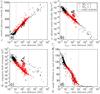 |
Fig. 9 Solar wind properties upstream of 850 extrasolar planets under consideration as a function of radial distance from the central star. a) Relative plasma velocity between stellar wind and planet; b) plasma density; c) magnetic field strength; d) angle Θ, i.e., deviation of magnetic field and relative plasma velocity from being perpendicular. Black dots are for Alfvén Mach numbers MA smaller than one and red dots are for MA > 1 (see also Fig. 10). |
In Fig. 9, we display the undisturbed stellar wind properties near the 850 extrasolar planets under consideration as function of radial distance from their central stars. This figure includes the relative plasma velocity v0 between the extrasolar planet and the stellar wind (Fig. 9a), the plasma density ρ (Fig. 9b), the magnetic field strength B0 (Fig. 9c), and the angle Θ between the normal to the magnetic field and the relative flow velocity (Fig. 9d) as a function of radial distance. Note that the Poynting flux is symmetric with respect to Θ = 90° (see also discussion in Sect. 2.2). The thin solid line displays the properties of the solar wind in the solar system. The black dots are for cases in which the stellar wind is sub-Alfvénic, i.e. MA < 1, and the red dots for MA > 1. In Fig. 10 we display the Alfvén Mach numbers MA near the 850 extrasolar planets as a function of radial distance calculated from the stellar wind properties shown in Fig. 9.
We find that the Alfvén Mach number distribution has a roughly similar dependency as expected from the Mach number in the solar wind shown as thin solid line in Fig. 10. The reason is that most known extrasolar planets orbit solar like stars. As expected MA < 1 is more likely to be met when an extrasolar planet is close to the star. We separate the extrasolar planets in three groups: an inner region close to the stars (rexo < 0.1 AU), an intermediate region (0.1 AU ≤ rexo < 10 AU), and an outer region (10 AU ≤ rexo). These regions are indicated as vertical lines in Figs. 9–11. Overall we find that 295 of the 850 planets under consideration are exposed to a stellar wind plasma with Alfvén Mach number MA less than one. We note that due to observational and model uncertainties and due natural temporal variations some extrasolar planets which are close to the MA = 1 line might shift from sub-Alfvénic to super-Alfvénic interaction and vice versa. In the inner region the probability for MA < 1 is the highest and is met by 234 out of 303 extrasolar planets. In the intermediate region it is fulfilled for 39 out of 519 and in the outer region for 22 out of 28 extrasolar planets.
For some extrasolar planets, MA lies significantly above the solar wind reference line, which contributes to cases with MA > 1. Most of the stars in the inner and intermediate region, where this is the case, belong to the stellar class M, which are color coded in red in Fig. 10. M type stars have small radii and masses compared to the sun and thus generate large stellar wind velocities within the Parker model. The smaller radii of M type stars also generate weaker stellar magnetic fields and thus smaller Alfvén velocities. Both effects contribute, on average, to larger values of MA compared to the solar case. The opposite holds for young-type stars. Extrasolar planets in the intermediate region with MA < 1 are possible in the opposite case, i.e. for large and young stars, which have a large rotation rate and thus a strong magnetic field (see Sect. 4.1). Yet observed extrasolar planets in the outer regions mostly orbit very young stars. Thus nearly all extrasolar planets in this region are, at first glance surprisingly, subject to a sub-Alfvénic plasma interaction. The currently most distant planet with MA < 1 is according to our model SR 12 AB c. As will be discussed below, many of these extrasolar planets, however, still cannot connect magnetically to the host star due to unsuitable directions of their Alfvén wings.
The total Poynting flux generated at each extrasolar planet where the interaction is
sub-Alfvénic is shown in Fig. 11 with the color code
displaying the stellar class of the central star. The values of the total Poynting flux
vary by many orders of magnitude and have a general tendency to decrease with radial
distance. For some of the extrasolar planets, our calculated stellar wind properties are
in a parameter space such that condition (56) is violated. In this case, we calculate a lower limit by decreasing the
interaction strength until
condition (56) is met. These cases are
displayed as circles in Fig. 11.
Large Poynting fluxes are observed for extrasolar planets very close to the central stars
and at radial distances around 1 AU, while the lowest Poynting fluxes are achieved for
planets around 0.1 AU. Within the studied ensemble of extra solar planets, no Poynting
flux arrives at the central star for rexo ≳ a few AU for
reasons to be discussed in the following paragraph. According to (55) the total Poynting flux is proportional
 . The
product of
. The
product of  decreases by roughly 15 orders of magnitude according to Fig. 9 within 0.01 and 1000 AU, which generates the decreasing trend with
radial distance. But the angular deviations Θ from the flow being perpendicular to the
stellar wind magnetic field also play a pronounced role (Fig. 9d). Near 0.1–0.3 AU we find a corridor with Θ ≈ 90° where
the flow and the magnetic field are nearly aligned with each other (Fig. 9d). In this corridor, cos2Θ ≈ 0 and the
motional electric field vanishes. Thus no or only very little Poynting flux is generated
in the interaction. This effect is responsible for the local minimum of the total Poynting
fluxes in the corridor between 0.1–0.3 AU displayed in Fig. 11. The effect of a vanishing motional electric field in this corridor was first
noticed in Zarka et al. (2001) and then applied in
Zarka (2007) to calculations of the energy
fluxes convected onto extrasolar planets. Particular large Poynting fluxes are also
observed for some extrasolar planets near 1 AU. This region is outside the “corridor”
region and the flow direction and the magnetic field direction are again sufficiently
different to generate large Poynting fluxes. The extrasolar planets in this region with
the largest Poynting fluxes orbit the largest stars of our ensemble of stars with an
interaction with MA < 1. These
extrasolar planets are also relative large in size and thus generate according to the
scaling law of (59) after Olson & Christensen (2006) large planetary
magnetic moments.
decreases by roughly 15 orders of magnitude according to Fig. 9 within 0.01 and 1000 AU, which generates the decreasing trend with
radial distance. But the angular deviations Θ from the flow being perpendicular to the
stellar wind magnetic field also play a pronounced role (Fig. 9d). Near 0.1–0.3 AU we find a corridor with Θ ≈ 90° where
the flow and the magnetic field are nearly aligned with each other (Fig. 9d). In this corridor, cos2Θ ≈ 0 and the
motional electric field vanishes. Thus no or only very little Poynting flux is generated
in the interaction. This effect is responsible for the local minimum of the total Poynting
fluxes in the corridor between 0.1–0.3 AU displayed in Fig. 11. The effect of a vanishing motional electric field in this corridor was first
noticed in Zarka et al. (2001) and then applied in
Zarka (2007) to calculations of the energy
fluxes convected onto extrasolar planets. Particular large Poynting fluxes are also
observed for some extrasolar planets near 1 AU. This region is outside the “corridor”
region and the flow direction and the magnetic field direction are again sufficiently
different to generate large Poynting fluxes. The extrasolar planets in this region with
the largest Poynting fluxes orbit the largest stars of our ensemble of stars with an
interaction with MA < 1. These
extrasolar planets are also relative large in size and thus generate according to the
scaling law of (59) after Olson & Christensen (2006) large planetary
magnetic moments.
An Alfvén Mach number less than one is, however, not a sufficient condition to establish
an electromagnetic coupling between an extrasolar planet and its central star. In several
cases, marked with crosses in Fig. 10,
MA is less than one, but the directions of both wings point
away from the star. This is the case when the stellar wind’s azimuthal magnetic field
component is large, i.e. the Parker magnetic field spiral is sufficiently wound up. Then
the two Alfvén wings are directed away from the star. This is for example the case for HD
11977 b as shown with the two red wings ( and
) in Fig.
12. In the same figure, we place a hypothetical
planet at closer radial distance to demonstrate the case when one wing points toward the
star (green dotted line) and thus electromagnetically couples to the star. For the wing
that couples to the star a phase lag between the exoplanet and its “footprint” on the star
is generated as discussed, e.g., in Preusse et al.
(2006) or Kopp et al. (2011). In case
where MA < 1 and both wings point away
from the star, the Poynting fluxes calculated with the full nonlinear expression (53) consistently lead to negative values and
are thus not shown in Fig. 11.
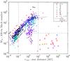 |
Fig. 10 Alfvén Mach number MA as a function of radial distance for the sample of 850 planets considered in this study. The spectral classes of the extrasolar planet hosting stars are color coded. The thin solid line represents MA in the solar wind of our solar system. Planets with MA < 1 whose wings still do not couple to the central star are marked with crosses (see text). |
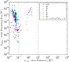 |
Fig. 11 Total Poynting fluxes carried in Alfvén wings as a function of distance from the
star for all 258 planets with sub-Alfvénic plasma interaction which connect to the
central star. The classes of the central stars are color coded. Planets marked with
a cross generate two Alfvén wings, which are both pointed away from the star and
thus do not connect to the central star. For extrasolar planets where condition
(56) is met, we accordingly lower
the interaction strength |
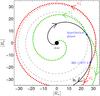 |
Fig. 12 Alfvén wings for HD 11977 b and a hypothetical planet at closer radial distance. Both Alfvén wings (in red) generated at HD 11977 b point away from the star and thus do not connect to it. A hypothetical planet at closer radial distance displays one wing that points toward the star and one wing away from it (shown in green). The black solid line displays a magnetic field line in the stellar wind and the dashed lines the orbital distances of the two planets. |
Overview of measured, estimated and calculated properties leading to the total Poynting flux of HD 179949 b.
Alfvén waves travel parallel to the magnetic field in the rest-frame of the unperturbed
plasma. The exact criterion that at least one wing points toward the star thus reads
 (60)i.e.,
the radial component of the relative velocity between the stellar wind and the planet
v0|r needs to be slower than the
radial component of the Alfvén velocity
(60)i.e.,
the radial component of the relative velocity between the stellar wind and the planet
v0|r needs to be slower than the
radial component of the Alfvén velocity  .
If the stellar wind is azimuthally symmetric, then the wing which points toward (away
from) the star will (not) connect to the star. For example, if the magnetic field
B0 is perpendicular to the radial stellar wind velocity
vsw, then the radial component of the Alfvén velocity is zero
and both wings always point away from the star (if vsw is
directed away from the star).
.
If the stellar wind is azimuthally symmetric, then the wing which points toward (away
from) the star will (not) connect to the star. For example, if the magnetic field
B0 is perpendicular to the radial stellar wind velocity
vsw, then the radial component of the Alfvén velocity is zero
and both wings always point away from the star (if vsw is
directed away from the star).
Note, that for extrasolar planets the central body is generally not located purely in the upstream direction of the relative flow because the relative velocity between the stellar wind and the planet generally possesses an azimuthal component due to the orbital velocity of the planet. Also note that condition (60) can be fulfilled if the interaction is super-Alfvénic, i.e. MA > 1. However, the theoretical model of the Alfvén wings applied in this paper is designed for sub-Alfvénic interaction only as the nature of the interaction changes for MA > 1.
The geometrical situation when both wings point away from the star is similar to the sub-Alfvénic interaction at the satellites of Jupiter and Saturn. At these satellites the magnetic field and the plasma flow are nearly perpendicular and thus the waves do not travel upstream, but are inclined toward the downstream direction. However, the central body, i.e. Jupiter and Saturn, are not upstream of the satellites, but nearly perpendicular to the flow direction and there is no (or only very little) relative velocity between the satellites and their central planets (in the radial and latitudinal direction).
The five extrasolar planets with the largest Poynting fluxes in decreasing order are WASP-12 b (3.1 × 10¹⁹ W), KOI-13 b (3.0 × 10¹⁹ W), WASP-78 b (1.4 × 10¹⁹ W), HD 208527 b (1.4 × 10¹⁹ W), WASP-33 b (1.4 × 10¹⁹ W). As supplementary information we provide the plasma properties and the calculated Poynting fluxes for all 850 extrasolar planets considered in this study in a Table available at the CDS. Our estimated stellar wind properties might be helpful for other studies of the interaction of extrasolar planets with their surrounding plasma environment. This table includes the names of the extrasolar planets, their distances from the host stars, the Kepler velocities of the extrasolar planets, the stellar wind velocities calculated with the Parker model, the radial and azimuthal components of the stellar wind magnetic fields, the stellar wind mass densities, the Alfvén Mach numbers, the total Poynting fluxes generated by the interaction, and details about the nature of the possible interactions and our calculations. The stellar wind properties provided in the online table are estimated near the vicinity of the extrasolar planets. Note, in many cases stellar properties are unknown and had to be estimated. Similarly, the existences, strengths and orientations of the magnetic moments of extrasolar planets are unknown. We used a scaling law to derive their magnetic moments which enter into our calculations of the total Poynting fluxes (see Sect. 4.1).
We also investigate if the kinetic or thermal energy flux can be positive toward the star with expressions (41) to (46) and find this is the case for only 8 of the extrasolar planets under consideration. These extrasolar planets are very close to the central star and the stellar wind magnetic field is still nearly radial. The resulting kinetic and thermal energy fluxes are, however, at least three orders of magnitude smaller compared to the respective Poynting fluxes and thus can be neglected.
In our calculations, the corona temperatures and the mass fluxes of the stars are assumed parameters based on typical values of our sun. We also studied how the number of extrasolar planets subject to sub-Alfvénic plasma flow and their resultant total Poynting fluxes vary if we, for example, increase the corona temperature to 2 × 10⁶ K or modify the coronal mass outflow by a factor of two. Even though individual values change, we find that the overall statistical distributions shown in Fig. 10 and Fig. 11 do not change qualitatively. For a factor of two larger/smaller mass fluxes, for example, the average Alfvén Mach number and the average total Poynting flux are somewhat enhanced/lowered, but still stay within the range of 1013 to 1020 W. According to Preusse et al. (2005) for a corona temperature of 2 × 10⁶ K, the differences between the stellar wind model after Parker (1958) and Weber & Davis (1967) become very small even for very fast rotating stars.
We note that not all of the energy in the Poynting flux generated at the extrasolar planets and traveling toward the central star will actually reach the central star. Part of the wave energy will be reflected/filamented in inhomogeneous plasma densities and magnetic fields or converted into heat and particle acceleration. Similar processes also occur to the Alfvén waves generated at the satellites of Jupiter and Saturn (Wright & Schwartz 1989; Chust et al. 2005; Jacobsen et al. 2007; Hess et al. 2010a).
The statistical study of the Poynting fluxes shows largely varying energy fluxes by many orders of magnitude. Only a few of the extrasolar planets generate energy fluxes on the order of 1019 W while the majority of the extrasolar planets generates fluxes many orders of magnitude smaller. These large variations are even seen within close radial distances of 0.1 AU. This could be a natural explanation why statistical studies of planet star interactions such as performed by Poppenhaeger et al. (2010) and Poppenhaeger & Schmitt (2011) do not find a statistically significant correlation between stellar emission and close-in extrasolar planets. Therefore strong and thus directly observable planet star coupling might only be possible for a few individual targets.
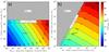 |
Fig. 13 Total Poynting flux generated at HD 179949 b as a function of a) stellar mass flow density F⋆ and planetary magnetic moment Mexo and b) stellar mass flow density F⋆ and field strength B⋆ with Mexo = 12MJ. The reference model with Mexo = 0.94MJ is calculated with scaling law (59) and labeled model; the reference model with Mexo = 12MJ is labeled model⋆. |
4.3. Poynting flux generated by HD 179949 b
Shkolnik et al. (2005) measure the excess energy flux in the chromospheric emission ascribed to magnetic planet star coupling for HD 179949 b to be ~1020 W. This value can be quantitatively compared with the calculations from Sect. 4.2. Table 3 gives an overview of the measured and estimated values to calculate the Poynting flux.
In the vicinity of HD 179949 b we calculate for the unperturbed stellar wind a relative velocity of 227 km s-1, a plasma density of 2.02 × 10⁻¹⁷ kg m-3, a magnetic field strength of 6870 nT, and the deviation of the flow from being perpendicular to the magnetic field of Θ = 115.7°. If we assume a dipole moment of HD 179949 b according to the scaling law in Eq. (59) of Mexo = 1.47 × 1027 A m2 which corresponds to a surface magnetic field of 4.25 × 10⁵ nT, we find that HD 179949 b generates a total Poynting flux of 3.36 × 10¹⁷ W. Here we assumed that the dipole moment is perpendicular to the stellar magnetic field (ΘM = 90°). Our value of the total Poynting flux is a factor of 2.5 higher compared to the estimate in Lanza (2009), but still a factor of ~300 smaller compared to the energies quoted in Shkolnik et al. (2005).
Because there are uncertainties of the used values, we explore parameter space to see
what conditions are required to achieve a Poynting flux on the order of 1020 W.
To calculate the total Poynting flux for HD 179949 b, we made assumptions on four
properties: the corona temperature T⋆, the
mass flow density F⋆ and magnetic field
B⋆ of the central star are not available
without assuming solar system values and/or scaling laws. As the existence and possible
strengths of intrinsic magnetic fields of extrasolar planets have not been observationally
demonstrated, the magnetic dipole moment Mexo of HD 179949 b
is also entirely uncertain. We thus investigate the influence of these four parameters. A
guide for the dependence of some of the parameters can be achieved by using the simplified
expression for the Poynting flux (55) and
the extension of the Alfvén wing (57)
which leads to 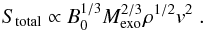 (61)Note
that the values in this expression describe the properties near the planet and not at the
star.
(61)Note
that the values in this expression describe the properties near the planet and not at the
star.
Our chosen stellar corona temperature already renders Poynting fluxes near its maximum value. A factor 10 lower value would cause a much weaker total energy flux of ~4 × 10¹² W. Assuming higher corona temperatures would basically lower the Poynting flux, too.
In Fig. 13a we show the total Poynting flux as
function of stellar mass flow density F⋆ and
planetary magnetic dipole moment Mexo. For high mass flow
densities there is a large parameter space where MA turns
larger than 1. The high plasma density ρ, resulting from high
F⋆, decreases the Alfvén velocity and
prohibits an energy flux directed to the central star. In a small interval of
F⋆ condition (56) is fulfilled. Here we approximate
Stotal with expression (55). For comparability the values of our standard model are marked
with a cross. In logarithmic presentation Stotal is a linear
function of the magnetic dipole moment as the Poynting flux scales with
 .
.
The surface magnetic field strength of HD 179949 b would need to be a factor of 4000 stronger than at Jupiter to explain a Poynting flux of 1020 W. Christensen et al. (2009) argue that extrasolar planets can have a magnetic field with a surface strength of 5–12 times the field strength of Jupiter. Using a factor of 12 the Poynting flux can not reach an order of 1020 W even with the assumption of a higher mass flow density. If F⋆ is a factor 10 higher than on the sun, the planetary magnetic moment still has to be a factor 500 stronger to produce a Poynting flux consistent with the energy fluxes quoted in Shkolnik et al. (2005). Because this is a rather unrealistic magnetic moment we look for other options to simulate the measurements. Varying B⋆ in our calculations linearly changes the stellar magnetic field near the extrasolar planet B0 and yields a weakly increasing energy flux with stronger magnetic fields (see Fig. 13 and Eq. (61)). The influence of B⋆ is too weak to achieve an order of 1020 W. The magnetic field would need to be a factor 100 stronger to reach only a slightly higher energy flux of ~1018 W. Note, our expressions for the Poynting fluxes even yield a weaker dependence on B0 compared to previous estimates with more simplified expressions of the local energetics (e.g., Lanza 2009). Figure 13b shows the dependency of the Poynting flux from stellar mass flow density F⋆ and magnetic field B⋆. To avoid exotic planetary properties, we set the magnetic dipole moment of HD179949 b equal to 12 times the field strength of Jupiter for this calculation. Next to this assumption F⋆ and B⋆ both still have to be at least a factor 100 higher, which is rather unlikely. Zarka (2007) and Lanza (2009) also come to similar conclusions that the observed fluxes by Shkolnik et al. (2005) require large or unrealistically large planetary and stellar fields, respectively, if the only energy source is the energy of the local interaction.
We also note that additionally not all the energy in the Poynting fluxes will be fully delivered to the star as the Alfvén waves experience filamentation and probably also scattering in a possibly turbulent stellar wind.
If the energy flux in the star planet interaction at HD 179949 b is indeed as strong as estimated by Shkolnik et al. (2005), then energy releases in coronal loops as suggested by Lanza (2009) might be an additional mean to produce the required energy. These releases, however, will be triggered and the associated planet star coupling will be energetically supplemented by the Alfvén waves launched at the planets calculated in this paper.
5. Conclusions and discussion
In this work we derive expressions for the Poynting flux in sub-Alfvénic plasma interaction, which can be applied to planetary moons in the outer solar system, but also to the coupling between extrasolar planets and their central stars. The expressions are calculated based on full nonlinear solutions of shear Alfvén waves within the framework of MHD (Neubauer 1980). We also provide simplified expressions for the total Poynting flux for small Alfvén Mach numbers (see Eqs. (54) or (55)), which are “user friendly” applicable, compared to our full expressions. Our expressions provide values for the Poynting flux generated near the planetary obstacles and thus likely present upper limits for the energy fluxes deposited into the central bodies since a fraction of the wave energy might be partially reflected or dissipated while traveling to the central bodies.
The flux values calculated in this work are consistent with footprint brightnesses observed at Jupiter’s moons Io, Europa, and Ganymede and Saturn’s moon Enceladus. We also model how the Poynting fluxes generated at the Galilean satellites vary as a function of system III in Jupiter’s magnetosphere.
We perform a statistical analysis on the existence and strength of magnetic planet star coupling based on all extrasolar planets known until 2012 November 14. We find that 295 of 850 extrasolar planets are embedded in a sub-Alfvénic, i.e. in an MA < 1 plasma environment. This is, however, only a necessary but not a sufficient condition that the Alfvénic interaction can transport energy upstream to the star. An additional requirement is that one of the two Alfvén wings generated in the interaction has a directional component toward the central star. This reduces the number of extrasolar planets within our ensemble which can magnetically couple to the star to 258. We find that the total Poynting fluxes generated at extrasolar planets in generally strongly decrease as a function of the planets distance from the central star within the first 0.1 AU. A local minimum of the flux is found near 0.1 AU because the local stellar wind magnetic field and the relative plasma velocities are often nearly parallel at theses distances (Zarka 2007).
Our modeled energy flux generated by HD 179949 b is more than two orders of magnitude smaller compared to the ~1020 W derived by Shkolnik et al. (2005). Only with rather exotically strong magnetic fields of the star HD 179949 and its companion values as derived by Shkolnik et al. (2005) can be achieved. The maximum modeled energy fluxes of our statistical study are on the order of 1019 W and thus still an order of magnitude smaller than the values derived by Shkolnik et al. (2005). If indeed observable planet star interaction requires energy fluxes on the order of 1020 W, then further energy sources are likely necessary. For example, the energy flux in the Alfvén waves originating at the extrasolar planets might trigger magnetic energy releases in coronal loops as suggested by Lanza (2009). In this case, still a threshold energy flux will be needed to trigger the additional release of coronal energy.
Our statistical analysis shows that the energy fluxes within the subset of extrasolar planets with MA < 1 vary by many orders of magnitudes even for the close-in extrasolar planets within 0.1 AU. Our findings might provide a natural explanation why statistical studies based on observations by Poppenhaeger et al. (2010) and Poppenhaeger & Schmitt (2011) find no statistical correlation between X-ray and optical luminosity of the stars and close-in extrasolar planets, but do not rule out the existence of electromagnetic planet star interaction for individual extrasolar planets.
Listed until 2012, November 14 on the website http://exoplanet.eu/
Acknowledgments
J.S. appreciates helpful discussions and comments by Peter Olson during his sabbatical stay at the Johns Hopkins University. J.S. also thanks Bertrand Bonfond and Sebastien Hess for helpful comments on the original manuscript. We thank Mario Seufert for providing values of his magnetic field model and Sven Jacobsen for providing density profiles of the Io plasma torus. Part of this work was supported by the German Deutsche Forschungsgemeinschaft, DFG with the Schwerpunktsprogramm Planetary Magnetism.
References
- Acuña, M. H., Neubauer, F. M., & Ness, N. F. 1981, J. Geophys. Res., 86, 8513 [NASA ADS] [CrossRef] [Google Scholar]
- Bagenal, F. 1994, J. Geophys. Res., 99, 11043 [NASA ADS] [CrossRef] [Google Scholar]
- Bagenal, F., & Delamere, P. A. 2011, J. Geophys. Res., 116, A05209 [NASA ADS] [CrossRef] [Google Scholar]
- Bigg, E. K. 1964, Nature, 203, 1008 [NASA ADS] [CrossRef] [Google Scholar]
- Bonfond, B. 2012, in Auroral Phenomenology and Magnetospheric Processes: Earth and Other Planets, eds. A. Keiling, et al. (Washington, D.C.: Geophys. Monogr. Ser.), 197, 133 [Google Scholar]
- Bonfond, B., Gérard, J.-C., Grodent, D., & Saur, J. 2007, Geophys. Res. Lett., 340, L06201 [NASA ADS] [CrossRef] [Google Scholar]
- Bonfond, B., Grodent, D., Gérard, J., et al. 2008, Geophys. Res. Lett., 35, L05107 [NASA ADS] [CrossRef] [Google Scholar]
- Bonfond, B., S., H., Gérard, J., et al. 2013, Planet. Space Sci., submitted [Google Scholar]
- Carroll, B. W., & Ostlie, D. A. 2007, in An introduction to modern astrophysics (San Francisco: Perason, Addion Wesley) [Google Scholar]
- Chané, E., Saur, J., Neubauer, F. M., Raeder, J., & Poedts, S. 2012, J. Geophys. Res., 117, 9217 [Google Scholar]
- Christensen, U. R., Holzwarth, V., & Reiners, A. 2009, Nature, 457, 167 [NASA ADS] [CrossRef] [PubMed] [Google Scholar]
- Chust, T., Roux, A., Kurth, W. S., et al. 2005, Plant. Space Sci., 53, 395 [Google Scholar]
- Clarke, J. T., Ballester, G. E., Trauger, J., et al. 1996, Science, 274, 404 [NASA ADS] [CrossRef] [Google Scholar]
- Clarke, J. T., Ballester, G. E., Trauger, J., et al. 1998, J. Geophys. Res., 103, 20217 [NASA ADS] [CrossRef] [Google Scholar]
- Clarke, J. T., Ajello, J., Ballester, G. E., et al. 2002, Nature, 415, 997 [NASA ADS] [CrossRef] [PubMed] [Google Scholar]
- Clarke, J. T. Benoit, C., Bradford, D., et al. 2011, in Magnetospheres of the Outer Planets, Boston, Massachusetts [Google Scholar]
- Cohen, O., Drake, J. J., Kashyap, V. L., et al. 2009, ApJ, 704, L85 [NASA ADS] [CrossRef] [Google Scholar]
- Connerney, J., Acuña, M. H., & Ness, N. F. 1982, J. Geophys. Res., 87, 3623 [NASA ADS] [CrossRef] [Google Scholar]
- Connerney, J. E. P., Baron, R., Satoh, T., & Owen, T. 1993, Science, 262, 1035 [NASA ADS] [CrossRef] [Google Scholar]
- Cuntz, M., Saar, S. H., & Musielak, Z. E. 2000, ApJ, 533, L151 [NASA ADS] [CrossRef] [PubMed] [Google Scholar]
- Dougherty, M. K., Khurana, K. K., Neubauer, F. M., et al. 2006, Science, 311, 1406 [NASA ADS] [CrossRef] [PubMed] [Google Scholar]
- Drell, S. D., Foley, H. M., & Ruderman, M. A. 1965, J. Geophys. Res., 70, 3131 [NASA ADS] [CrossRef] [Google Scholar]
- Elsässer, W. 1950, Phys. Rev., 79, 183 [NASA ADS] [CrossRef] [Google Scholar]
- Frank, L. A., Paterson, W. R., Ackerson, K. L., et al. 1996, Science, 274, 394 [Google Scholar]
- Gérard, J.-C., Saglam, A., Grodent, D., & Clarke, J. 2006, J. Geophys. Res., 111, A04202 [NASA ADS] [CrossRef] [Google Scholar]
- Goertz, C. K. 1980, J. Geophys. Res., 85, 2949 [Google Scholar]
- Goldreich, P., & Lynden-Bell, D. 1969, ApJ, 156, 59 [NASA ADS] [CrossRef] [Google Scholar]
- Grießmeier, J., Stadelmann, A., Penz, T., et al. 2004, A&A, 425, 753 [NASA ADS] [CrossRef] [EDP Sciences] [Google Scholar]
- Grießmeier, J., Motschmann, U., Mann, G., & Rucker, H. O. 2005, A&A, 437, 717 [NASA ADS] [CrossRef] [EDP Sciences] [Google Scholar]
- Grießmeier, J., Zarka, P., & Spreeuw, H. 2007, A&A, 475, 359 [NASA ADS] [CrossRef] [EDP Sciences] [Google Scholar]
- Grodent, D., Gérard, J., Gustin, J., et al. 2006, Geophys. Res. Lett., 33, L6201 [NASA ADS] [CrossRef] [Google Scholar]
- Grodent, D., Bonfond, B., Radioti, A., et al. 2009, J. Geophys. Res., 114, 07212 [Google Scholar]
- Gustin, J., Bonfond, B., Grodent, D., & Gérard, J.-C. 2012, J. Geophys. Res., 117, 7316 [CrossRef] [Google Scholar]
- Hess, S. L. G., & Zarka, P. 2011, A&A, 531, A29 [NASA ADS] [CrossRef] [EDP Sciences] [Google Scholar]
- Hess, S. L. G., Delamere, P., Dols, V., Bonfond, B., & Swift, D. 2010a, J. Geophys. Res., 115, 06205 [CrossRef] [Google Scholar]
- Hess, S., Bonfond, B., Delamere, P. A., et al. 2010b, AGU Fall Meeting Abstracts, C1775 [Google Scholar]
- Hess, S. L. G., Delamere, P. A., Dols, V., & Ray, L. C. 2011a, J. Geophys. Res. Space Phys., 116, A01202 [NASA ADS] [CrossRef] [Google Scholar]
- Hess, S. L. G., Delamere, P. A., Bagenal, F., Schneider, N., & Steffl, A. J. 2011b, J. Geophys. Res., 116, 11215 [CrossRef] [Google Scholar]
- Hess, S. L. G., et al. 2013, Plant. Space Sci., submitted [Google Scholar]
- Ip, W.-H., Kopp, A., & Hu, J. 2004, ApJ, 602, L53 [NASA ADS] [CrossRef] [Google Scholar]
- Jacobsen, S. 2011, Dissertation, Institut für Geophysik und Meteorologie, Universität zu Köln [Google Scholar]
- Jacobsen, S., Neubauer, F. M., Saur, J., & Schilling, N. 2007, Geophys. Res. Lett., 34, 10202 [NASA ADS] [CrossRef] [Google Scholar]
- Jacobsen, S., Saur, J., Neubauer, F. M., et al. 2010, J. Geophys. Res., 115, 4205 [CrossRef] [Google Scholar]
- Jia, X., Walker, R., Kivelson, M., Khurana, K., & Linker, J. 2009, J. Geophys. Res., 114, 09209 [Google Scholar]
- Jia, Y.-D., Russell, C. T., Khurana, K. K., et al. 2010, J. Geophys. Res., 115, 04214 [CrossRef] [Google Scholar]
- Khurana, K. K., Dougherty, M. K., Russell, C. T., & Leisner, J. S. 2007, J. Geophys. Res., 112, A8 [CrossRef] [Google Scholar]
- Kivelson, M. G., Khurana, K. K., Russell, C. T., et al. 1996a, Nature, 384, 537 [NASA ADS] [CrossRef] [Google Scholar]
- Kivelson, M. G., Khurana, K. K., Walker, R. J., et al. 1996b, Science, 273, 337 [NASA ADS] [CrossRef] [Google Scholar]
- Kivelson, M. G., Bagenal, F., Neubauer, F. M., et al. 2004, in Jupiter, ed. F. Bagenal (University of Colorado: Cambridge Univ. Press), 513 [Google Scholar]
- Kopp, A., Schilp, S., & Preusse, S. 2011, ApJ, 729, 116 [NASA ADS] [CrossRef] [Google Scholar]
- Kriegel, H., Simon, S., Müller, J., et al. 2009, Planet. Space Sci., 57, 2113 [NASA ADS] [CrossRef] [Google Scholar]
- Kriegel, H., Simon, S., Motschmann, U., et al. 2011, J. Geophys. Res., 116, 10223 [CrossRef] [Google Scholar]
- Lanza, A. F. 2008, A&A, 487, 1163 [NASA ADS] [CrossRef] [EDP Sciences] [Google Scholar]
- Lanza, A. F. 2009, A&A, 505, 339 [NASA ADS] [CrossRef] [EDP Sciences] [Google Scholar]
- Li, J., Ferrario, L., & Wickramasinghe, D. 1998, ApJ, 503, L151 [NASA ADS] [CrossRef] [Google Scholar]
- Lindal, G. F., Wood, G. E., Levy, G. S., et al. 1981, J. Geophys. Res., 86, 8721 [NASA ADS] [CrossRef] [Google Scholar]
- Lipatov, A. S., Motschmann, U., Bagdonat, T., & Grießmeier, J. 2005, Planet. Space Sci., 53, 423 [NASA ADS] [CrossRef] [Google Scholar]
- Lockwood, M., Stamper, R., & Wild, M. N. 1999, Nature, 399, 437 [NASA ADS] [CrossRef] [Google Scholar]
- Neubauer, F. M. 1980, J. Geophys. Res., 85, 1171 [Google Scholar]
- Neubauer, F. M. 1998, J. Geophys. Res., 103, 19843 [Google Scholar]
- Newkirk, Jr., G. 1980, in The Ancient Sun: Fossil Record in the Earth, Moon and Meteorites, eds. R. O. Pepin, J. A. Eddy, & R. B. Merrill, 293 [Google Scholar]
- Olson, P., & Christensen, U. R. 2006, Earth Planet. Sci. Lett., 250, 561 [NASA ADS] [CrossRef] [Google Scholar]
- Parker, E. N. 1958, ApJ, 128, 664 [Google Scholar]
- Piddington, J. H., & Drake, J. F. 1968, Nature, 217, 935 [NASA ADS] [CrossRef] [Google Scholar]
- Poppenhaeger, K., & Schmitt, J. H. M. M. 2011, ApJ, 735, 59 [NASA ADS] [CrossRef] [Google Scholar]
- Poppenhaeger, K., Robrade, J., & Schmitt, J. 2010, A&A, 515, A98 [NASA ADS] [CrossRef] [EDP Sciences] [Google Scholar]
- Poppenhaeger, K., Lenz, L. F., Reiners, A., Schmitt, J. H. M. M., & Shkolnik, E. 2011, A&A, 528, A58 [NASA ADS] [CrossRef] [EDP Sciences] [Google Scholar]
- Prangé, R., Rego, D., Southwood, D., et al. 1996, Nature, 379, 323 [NASA ADS] [CrossRef] [Google Scholar]
- Preusse, S., Kopp, A., Büchner, J., & Motschmann, U. 2005, A&A, 434, 1191 [NASA ADS] [CrossRef] [EDP Sciences] [Google Scholar]
- Preusse, S., Kopp, A., Büchner, J., & Motschmann, U. 2006, A&A, 460, 317 [NASA ADS] [CrossRef] [EDP Sciences] [Google Scholar]
- Preusse, S., Kopp, A., Büchner, J., & Motschmann, U. 2007, Plant. Space Sci., 55, 589 [Google Scholar]
- Pryor, W. R., Rymer, A. M., Mitchell, D. G., et al. 2011, Nature, 472, 331 [NASA ADS] [CrossRef] [Google Scholar]
- Roussos, E., Krupp, N., Armstrong, T. P., et al. 2008, Geophys. Res. Lett., 352, L22106 [NASA ADS] [CrossRef] [Google Scholar]
- Santolík, O., Gurnett, D. A., Jones, G. H., et al. 2011, Geophys. Res. Lett., 38, 19204 [NASA ADS] [Google Scholar]
- Saur, J. 2004, J. Geophys. Res., 109, A01210 [Google Scholar]
- Saur, J., & Strobel, D. F. 2005, ApJ, 620, L115 [NASA ADS] [CrossRef] [Google Scholar]
- Saur, J., Strobel, D. F., & Neubauer, F. M. 1998, J. Geophys. Res., 103, 19947 [Google Scholar]
- Saur, J., Neubauer, F. M., Strobel, D. F., & Summers, M. E. 1999, J. Geophys. Res., 104, 25105 [NASA ADS] [CrossRef] [Google Scholar]
- Saur, J., Neubauer, F. M., Strobel, D. F., & Summers, M. E. 2002, J. Geophys. Res., 107, 1422 [Google Scholar]
- Saur, J., Neubauer, F. M., & Schilling, N. 2007, J. Geophys. Res., 112, A11209 [NASA ADS] [CrossRef] [Google Scholar]
- Saur, J., Schilling, N., Neubauer, F. M., et al. 2008, Geophys. Res. Lett., 35, L20105 [NASA ADS] [CrossRef] [Google Scholar]
- Scharf, C. A. 2010, ApJ, 722, 1547 [NASA ADS] [CrossRef] [Google Scholar]
- Schilling, N. 2006, Dissertation, Institut für Geophysik und Meteorologie der Universität zu Köln [Google Scholar]
- Schneider, J., Dedieu, C., Le Sidaner, P., Savalle, R., & Zolotukhin, I. 2011, ArXiv e-prints [Google Scholar]
- Schwenn, R. 1990, in Physics of the Inner Heliosphere I, eds. R. Schwenn, & E. Marsch (Berlin: Springer), 99 [Google Scholar]
- Seufert, M., Saur, J., & Neubauer, F. M. 2011, Icarus, 214, 477 [NASA ADS] [CrossRef] [Google Scholar]
- Shkolnik, E., Walker, G. A. H., & Bohlender, D. A. 2003, ApJ, 597, 1092 [NASA ADS] [CrossRef] [Google Scholar]
- Shkolnik, E., Walker, G. A. H., Bohlender, D. A., Gu, P., & Kürster, M. 2005, ApJ, 622, 1075 [NASA ADS] [CrossRef] [Google Scholar]
- Shkolnik, E., Bohlender, D. A., Walker, G. A. H., & Collier Cameron, A. 2008, ApJ, 676, 628 [NASA ADS] [CrossRef] [Google Scholar]
- Simon, S., Saur, J., Neubauer, F. M., Motschmann, U., & Dougherty, M. K. 2009, Geophys. Res. Lett., 360, L04108 [NASA ADS] [CrossRef] [Google Scholar]
- Simon, S., Saur, J., Kriegel, H., et al. 2011a, J. Geophys. Res., 116, A04221 [NASA ADS] [CrossRef] [Google Scholar]
- Simon, S., Saur, J., Neubauer, F. M., Wennmacher, A., & Dougherty, M. K. 2011b, Geophys. Res. Lett., 381, L15102 [NASA ADS] [Google Scholar]
- Simon, S., Kriegel, H., Saur, J., et al. 2012, J. Geophys. Res., 117, 7211 [CrossRef] [Google Scholar]
- Strobel, D. F., Saur, J., Feldman, P. D., & McGrath, M. A. 2002, ApJ, 581, L51 [NASA ADS] [CrossRef] [Google Scholar]
- Teolis, B. D., Jones, G. H., Miles, P. F., et al. 2010, Science, 330, 1813 [NASA ADS] [CrossRef] [Google Scholar]
- Tokar, R., Johnson, R. E., Hill, T. W., et al. 2006, Science, 311, 1409 [NASA ADS] [CrossRef] [PubMed] [Google Scholar]
- Wang, Y.-M., & Sheeley, Jr., N. R., 1995, ApJ, 447, L143 [NASA ADS] [Google Scholar]
- Wannawichian, S., Clarke, J. T., & Nichols, J. D. 2010, J. Geophys. Res., 115, A02206 [NASA ADS] [CrossRef] [Google Scholar]
- Weber, E. J., & Davis, Jr., L., 1967, ApJ, 148, 217 [NASA ADS] [CrossRef] [Google Scholar]
- Willes, A. J., & Wu, K. 2004, MNRAS, 348, 285 [NASA ADS] [CrossRef] [Google Scholar]
- Willes, A. J., & Wu, K. 2005, A&A, 432, 1091 [NASA ADS] [CrossRef] [EDP Sciences] [Google Scholar]
- Wright, A. N., & Schwartz, S. J. 1989, J. Geophys. Res., 94, 3749 [NASA ADS] [CrossRef] [Google Scholar]
- Zarka, P. 1998, J. Geophys. Res., 103, 20159 [NASA ADS] [CrossRef] [Google Scholar]
- Zarka, P. 2006, in Planetary Radio Emission VI, eds. H. O. Rucker, W. S. Kurth, & G. Mann (Austria: Austrian Academy of Sciences Press), 543 [Google Scholar]
- Zarka, P. 2007, Plant. Space Sci., 55, 598 [NASA ADS] [CrossRef] [Google Scholar]
- Zarka, P., Treumann, R. A., Ryabov, B. P., & Ryabov, V. B. 2001, Ap&SS, 277, 293 [Google Scholar]
All Tables
Total Poynting fluxes and properties at satellites for average magnetospheric values.
Overview and classification of the 850 extrasolar planets and their associated stars under consideration according to (a) stellar class and Alfvén Mach number and (b) applied strategies when not all stellar properties to model the stellar wind are available.
Overview of measured, estimated and calculated properties leading to the total Poynting flux of HD 179949 b.
All Figures
|
Fig. 1 Geometrical properties of the interaction of a planetary body with its
surrounding magnetized plasma with B0: unperturbed stellar
wind magnetic field, vsw: stellar wind velocity,
vorbit: orbital velocity of planet,
v0: relative velocity between planet and stellar wind
plasma, Mexo: magnetic moment of planet (in this figure it
points out of the displayed plane), |
| In the text | |
|
Fig. 2 Sketch of the Alfvén wing and its associated dissipation region for idealized stellar wind properties in a frame of reference rotating with the central body. The idealized orientations of the vector fields in the sketch resemble the situation when the radius of the star R⋆ is much larger than the effective radius of the extra solar planet Reff and the angular velocity of the star, the radial distance of the extra solar planet and the stellar wind velocity obey Ω⋆rexo/vsw ≪ 1. The sketch displays the wing at time t and also indicates the time-variability of the wing in the rotating frame. At time t the extra solar planet is situated at a location marked with a brown circle. The extra solar planet in this frame of reference was located at earlier times t − Δt further to the right. The extra solar planet steadily launches Alfvén waves, which travel parallel to B0. The superposition of the wave packets launched at earlier times results in the snapshot of the wing at time t displayed here. |
| In the text | |
|
Fig. 3 Poynting flux through a plane perpendicular to B0 for
Alfvén Mach number MA = 0.8, interaction strength
|
| In the text | |
|
Fig. 4 Total Poynting flux through a plane perpendicular to B0 as
a function of the interaction strength |
| In the text | |
|
Fig. 5 Total Poynting flux as a function of the angle Θ between the background magnetic
field B0 and the incident plasma velocity
v0. The angle Θ is zero, when B0
and v0 are perpendicular (see Fig. 1). The Poynting flux is symmetric with respect to 90°.
For the planetary bodies under consideration in this work, Θ falls into the range
0 ≤ Θ ≤ 180°. Note that in this figure, we additionally show the range
− 90° ≤ Θ ≤ 0° for cases where such an orientation of the
magnetic field and the velocity occur. The interaction strength and the Alfvén Mach
number are chosen as |
| In the text | |
|
Fig. 6 Magnetic field topology and effective radius of Alfvén wings for oblique intrinsic and exterior field orientations. White dotted lines show magnetic field lines and black arrows indicate the magnetic field direction. The field strength is displayed color coded. The boundary, which separates closed field lines starting and ending on the planet from field lines connecting to the star, are displayed as solid white line. The distance of these field lines at larger distance from the planet establishes the effective diameter Deff of the Alfvén wings. |
| In the text | |
|
Fig. 7 Effective radius of Alfvén wing in units of Robst (see (57)) as a function of the orientation of the intrinsic to the external magnetic field (solid line). Two analytical approximations are shown as dashed and dotted lines. |
| In the text | |
|
Fig. 8 Total Poynting flux generated by the Galilean satellites as a function of system
III longitude for different models of the plasma density and interaction strength.
Solid lines display the Poynting flux with magnetospheric density models after Bagenal & Delamere (2011) calculated with
two different assumptions of the interaction strength
|
| In the text | |
|
Fig. 9 Solar wind properties upstream of 850 extrasolar planets under consideration as a function of radial distance from the central star. a) Relative plasma velocity between stellar wind and planet; b) plasma density; c) magnetic field strength; d) angle Θ, i.e., deviation of magnetic field and relative plasma velocity from being perpendicular. Black dots are for Alfvén Mach numbers MA smaller than one and red dots are for MA > 1 (see also Fig. 10). |
| In the text | |
|
Fig. 10 Alfvén Mach number MA as a function of radial distance for the sample of 850 planets considered in this study. The spectral classes of the extrasolar planet hosting stars are color coded. The thin solid line represents MA in the solar wind of our solar system. Planets with MA < 1 whose wings still do not couple to the central star are marked with crosses (see text). |
| In the text | |
|
Fig. 11 Total Poynting fluxes carried in Alfvén wings as a function of distance from the
star for all 258 planets with sub-Alfvénic plasma interaction which connect to the
central star. The classes of the central stars are color coded. Planets marked with
a cross generate two Alfvén wings, which are both pointed away from the star and
thus do not connect to the central star. For extrasolar planets where condition
(56) is met, we accordingly lower
the interaction strength |
| In the text | |
|
Fig. 12 Alfvén wings for HD 11977 b and a hypothetical planet at closer radial distance. Both Alfvén wings (in red) generated at HD 11977 b point away from the star and thus do not connect to it. A hypothetical planet at closer radial distance displays one wing that points toward the star and one wing away from it (shown in green). The black solid line displays a magnetic field line in the stellar wind and the dashed lines the orbital distances of the two planets. |
| In the text | |
|
Fig. 13 Total Poynting flux generated at HD 179949 b as a function of a) stellar mass flow density F⋆ and planetary magnetic moment Mexo and b) stellar mass flow density F⋆ and field strength B⋆ with Mexo = 12MJ. The reference model with Mexo = 0.94MJ is calculated with scaling law (59) and labeled model; the reference model with Mexo = 12MJ is labeled model⋆. |
| In the text | |
Current usage metrics show cumulative count of Article Views (full-text article views including HTML views, PDF and ePub downloads, according to the available data) and Abstracts Views on Vision4Press platform.
Data correspond to usage on the plateform after 2015. The current usage metrics is available 48-96 hours after online publication and is updated daily on week days.
Initial download of the metrics may take a while.