| Issue |
A&A
Volume 551, March 2013
|
|
|---|---|---|
| Article Number | A51 | |
| Number of page(s) | 9 | |
| Section | Planets and planetary systems | |
| DOI | https://doi.org/10.1051/0004-6361/201219903 | |
| Published online | 20 February 2013 | |
A new model for the ν1 vibrational band of HCN in cometary comae, with application to three comets⋆
1
Max Planck Institute for Solar System Research,
Katlenburg-Lindau,
Germany
e-mail:
This email address is being protected from spambots. You need JavaScript enabled to view it.
2
The Goddard Center for Astrobiology, NASA Goddard Space Flight
Center, Greenbelt,
MD, 20771, USA
3
Department of Geophysics and Planetary Sciences, Tel Aviv
University, Tel Aviv,
Israel
4
Dept. of Physics, Catholic University of
America, Washington
DC, 20064, USA
Received:
26
June
2012
Accepted:
28
December
2012
Abstract
Aims. Hydrogen cyanide (HCN) radiates effectively at infrared wavelengths in cometary atmospheres, and a new quantum-band model is needed to properly interpret high-resolution spectra. HCN spectra of comets 8P/Tuttle, C/2007 W1 (Boattini), and C/2008 Q3 (Garradd) have been recorded by our team using the high-resolution CRyogenic InfraRed Echelle Spectometer (CRIRES) at the Very Large Telescope (VLT), ultimately posing an excellent test for our newly developed model.
Methods. We developed a quantum-band model for the ν1 fundamental of HCN using the latest spectroscopic parameters available and with it retrieved HCN in the above mentioned three comets. For each comet, we sampled several lines of HCN in the spectral region near 3 μm, and retrieved molecular production rates, mixing ratios, and rotational temperatures.
Results. When compared to other comets, 8P/Tuttle is relatively depleted in HCN, while C/2007 W1 (Boattini) appears to be enriched and C/2008 Q3 (Garradd) normal. The spatial profile of HCN observed in 8P/Tuttle is symmetric, consistent with isotropic outgassing from the nucleus, while in comet C/2007 W1 we observed an asymmetric excess of HCN in the anti-solar direction. We investigated the HCN-CN parentage by comparing our production rate ratios (HCN/H2O) with those of CN/OH derived at optical wavelengths. In comet C/2007 W1 the two mixing ratios are comparable, while in 8P/Tuttle our derived HCN abundance is too low to support the HCN molecule as the only parent of the CN radical.
Key words: molecular data / astrobiology / comets: individual: 8P/Tuttle / comets: individual: C/2007W1 (Boattini) / infrared: general / comets: individual: C/2008 Q3 (Garradd)
Based on observations obtained at the ESO – European Southern Observatory at Cerro Paranal, Chile, under programs 080.C-0257(A), 081.C-0116(A), 083.C-0646(A).
© ESO, 2013
1. Introduction
Comets are considered to be among the least processed bodies of the solar system, and their compositions may reveal critical information about the diverse conditions that were present in the proto-planetary nebula, the place and the time where and when they formed. A taxonomy based on the chemical composition of these bodies could test a possible radial gradient in the chemistry of icy planetesimals in the proto-planetary disk, along with the dynamical models that predict their dissemination. As sublimating volatiles are released in cometary comae, they radiate effectively in the infrared via solar-induced fluorescence. The analysis of this emission using high-resolution spectroscopy (resolving power ≥20 000) in the mid-IR (3–5 μm) permits the sampling of the chemical and physical properties of cometary volatiles with high sensitivity.
Today, the increasing capabilities of telescopes and instruments allow us to observe the inner part of a cometary coma with unprecedented high spatial and spectral resolution. To properly interpret these spectra, advanced molecular models that compute fluorescence emission efficiencies are necessary to convert the measured line fluxes to molecular production rates. These models require a precise description of the rotational structure of all vibrational levels involved, together with accurate statistical weights, selection rules, perturbations (e.g. Coriolis effects, splittings, tunneling) and band-emission rates.
We present a new fluorescence model of the ν1 ro-vibrational fundamental band of HCN and use this to retrieve production rates, mixing ratios relative to water, and rotational temperatures in three comets observed by our team at the Very Large Telescope (VLT). The model can be extended to other species to correctly interpret cometary spectra obtained using high-dispersion spectroscopy.
2. HCN fluorescence model
2.1. The importance of HCN in cometary studies
Hydrogen cyanide (HCN) is a typical component present in cometary ices that may have played an important role in the development of life on our planet. HCN could have been deposited on Earth by comets, meteorites, and interplanetary dust particles, giving rise to essential polymeric structures, and, in presence of liquid water, to formation of amino acids and proteins and ultimately to life as we know it (Matthews & Minard 2008).
Comparison of HCN abundances in comets with those observed in the interstellar medium can be used to investigate the primordial conditions of our solar system, while the relative abundance among nitrogen-bearing molecules in comets (HCN, NH3, N2, etc.) may be indicative of the formation temperature and the kind and degree of processing experienced by pre-cometary material, whether in the natal cloud or in the solar nebula (Mumma et al. 1993; Mumma & Charnley 2011).
HCN is a linear molecule with a triple bond between carbon and nitrogen, and it is characterized by three normal vibrational modes: C-H stretching, C-N stretching, and H-C-N bending. Emission lines in cometary comae related to the C-H stretching mode can be easily observed in the IR spectral region, at about 3.3 μm.
2.2. The model
Currently, the increasing capability of infrared telescopes and instrumentation enables astronomical sensing with unprecedented sensitivity, and with spectral resolution sufficient to reveal the rotational structure of vibrational bands emitted by molecules in the inner cometary coma. With this higher precision, it becomes essential to employ improved fluorescence models that can fully interpret the observed spectra.
Fluorescence is a non-LTE (non local thermal equilibrium) process, and for this reason it cannot be simply described using values tabulated in terrestrial line atlases that are suitable for an LTE regime (e.g., HITRAN Rothman et al. 2009). If the goal is to correctly reproduce the observed emissions, it is fundamental to build a complete quantum mechanical model, which is more suitable to describing this physical process. Previous models for synthesizing HCN spectra (Crovisier 1987; Magee-Sauer et al. 1999; Mumma et al. 2001) are valuable tools for this analysis, and building on them we have developed a new model for HCN that incorporates the latest spectroscopic data.
First of all, our new model reproduces more reliable line-by-line fluorescence efficiencies (g-factors), beginning with the precise knowledge of the rotational structure for each vibrational level involved. Using information contained in the latest HITRAN compilation (Rothman et al. 2009), we have re-built the ro-vibrational structure of the HCN molecule and computed all other necessary parameters, including the Einstein A-coefficients for spontaneous emission. By doing so, we retain complete control of the model parameters. Moreover, with this method we are able to include the latest updated molecular band parameters (see Table 1), and to include in the computation various perturbations (e.g., Coriolis effects, level splittings, and tunneling) that were not considered in previous models.
The solar flux received by the comet is another important factor. Our previous model approximated the wavelength-dependent solar flux by a blackbody spectrum. However, the fluorescence excitation of a ro-vibrational band depends on the absolute solar flux that excites the molecule, so the approximation by a simple blackbody (Planck function) may lead to inaccurate pumping calculations. For this reason we used a more realistic solar spectrum, obtained by convolving a continuum model (Kurucz 1997) with the accurate Hase solar atlas (Hase et al. 2006), which consists of an empirical detailed line-by-line model of the solar transmittance spectrum (details of this solar model are described in Appendix B of Villanueva et al. 2011b). This solar model also takes into account the presence of Fraunhofer absorption lines in the solar spectrum, requiring the calculation of g-factors for the corresponding heliocentric velocity of the comet (Swings 1941). Omitting the Swings effect will lead to incorrect retrievals of rotational temperatures, since these are derived from measured line-by-line intensities after correcting for the solar pumping flux.
Collision partners in cometary atmospheres usually lack sufficient energy to excite vibrational transitions, and the rate of quenching collisions is much lower than radiative decay rates for (infrared-active) excited states. Thus, the vibrational manifold is not populated in LTE. Instead, solar radiation pumps the molecules into an excited vibrational state, which then de-excites by rapid radiative decay. Infrared photons are emitted through decay to the ground-vibrational state either directly (resonant fluorescence) or through branching into intermediate vibrational levels (non-resonant fluorescence). Optical pumping in the ν1 band is the expected dominant factor in the excitation of this band in comets, and it is the sole pumping mechanism we consider here, although additional excitation cascading from levels with energies higher than ν1 may also contribute, albeit in a minor way.
Knowledge of the initial (or equilibrium) population in the ground-vibrational state is fundamental when computing the pumping rates into individual rotational levels in the upper vibrational state of interest; since collisions dominate radiative decay in the pure rotational transitions, we can assume a rotational temperature Trot to describe the rotational population (Xie & Mumma 1992).
Using the appropriate selection rules, the frequencies of the allowed transitions between
the two vibrational levels involved (ground and ν1) are
computed as  (1)where
ν0 is the frequency of the pure vibrational transition, and
Elow and Eup are given by
(1)where
ν0 is the frequency of the pure vibrational transition, and
Elow and Eup are given by
 (2)In
Eq. (2), the subscripts “low” and “up”
refer to the lower and upper vibrational levels, Blow and
Bup are the rotational constants, J is the
rotational angular momentum quantum number (which takes integer positive numbers,
J = 0,1,2, etc.);
Dlow, Dup,
Hlow, and Hup are the second and
third rotational constants for the second- and third- order corrections. Values of the
rotational constants and ν0 in Eqs. (1) and (2) were derived in the laboratory by performing highly precise spectroscopic
measurements of several ro-vibrational bands. See band constants and corresponding
references in Table 1.
(2)In
Eq. (2), the subscripts “low” and “up”
refer to the lower and upper vibrational levels, Blow and
Bup are the rotational constants, J is the
rotational angular momentum quantum number (which takes integer positive numbers,
J = 0,1,2, etc.);
Dlow, Dup,
Hlow, and Hup are the second and
third rotational constants for the second- and third- order corrections. Values of the
rotational constants and ν0 in Eqs. (1) and (2) were derived in the laboratory by performing highly precise spectroscopic
measurements of several ro-vibrational bands. See band constants and corresponding
references in Table 1.
Constants used for the HCN-ν1 model.
To compute the rotational line intensities, we partitioned the band intensity along the R and P branches by scaling by the corresponding Hönl-London factor LJ and the fractional population of the lower state energy (including self-emission, see Eq. (3)). We also compensated for rotational-vibrational interactions by means of the Herman-Wallis factor F. In our model, we computed LJ using the expression L = m2/|m |,with m = J(J + 1) for the R-branch and m = −J for the P-branch, while for F we used the approximation F = (1 + A1m)2, with m defined as before (for both equations see Malathy Devi et al. 2003, and references therein); the parameter A1 was measured in the laboratory and its value is listed in Table 1.
The rotational line intensities were then computed as in Malathy Devi et al. (2003): ![Mathematical equation: \begin{equation} S_{lu} = \frac{\nu}{\nu_{0}}L_{J}\frac{S_{\rm v}}{Q_{\rm r}}{\rm e}^{-c_{2}E_{\mathrm{low}}/T_{\mathrm{rot}}}\left[1-{\rm e}^{-c_{2}\nu/T_{\mathrm{rot}}}\right]F; \label{eq3} \end{equation}](/articles/aa/full_html/2013/03/aa19903-12/aa19903-12-eq57.png) (3)here,
Qr is the rotational partition function at the rotational
temperature Trot,
c2 = hc/k,
and Sv is the vibrational band intensity. The value for
Sv, listed in Table 1, was measured in the laboratory for a standard temperature of 296 K, but it is
possible to convert it to any temperature T (see for example Šimečková et al. 2006). The rotational partition
function is given by
(3)here,
Qr is the rotational partition function at the rotational
temperature Trot,
c2 = hc/k,
and Sv is the vibrational band intensity. The value for
Sv, listed in Table 1, was measured in the laboratory for a standard temperature of 296 K, but it is
possible to convert it to any temperature T (see for example Šimečková et al. 2006). The rotational partition
function is given by 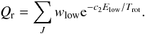 (4)We directly computed the
Einstein coefficients for spontaneous emission
Aul following Šimečková et al. (2006):
(4)We directly computed the
Einstein coefficients for spontaneous emission
Aul following Šimečková et al. (2006): 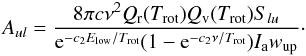 (5)In Eq. (5),
Qv(Trot) is the vibrational
partition function, which for simplicity was assumed to be 1,
wup is the degeneracy of the upper state, and
Ia is the isotopic ratio for the HCN molecule (we adopted
the terrestrial value, see Table 1). The Einstein
coefficient for absorption Blu is related to
the Einstein coefficients for spontaneous emission
Aul by the following equation:
(5)In Eq. (5),
Qv(Trot) is the vibrational
partition function, which for simplicity was assumed to be 1,
wup is the degeneracy of the upper state, and
Ia is the isotopic ratio for the HCN molecule (we adopted
the terrestrial value, see Table 1). The Einstein
coefficient for absorption Blu is related to
the Einstein coefficients for spontaneous emission
Aul by the following equation:
 (6)If
Jν is the solar flux received by the
comet at frequency ν, the total pumping g-factor for a
ro-vibrational level u is
(6)If
Jν is the solar flux received by the
comet at frequency ν, the total pumping g-factor for a
ro-vibrational level u is
 (7)where
wlow is the degeneracy of the lower state; for each line, we
took the value for Jν retrieved from the
adopted solar model described before.
(7)where
wlow is the degeneracy of the lower state; for each line, we
took the value for Jν retrieved from the
adopted solar model described before.
Once all pump factors were computed, the cometary fluorescence rates, i.e., the
g-factors, are given by
 (8)where
Aul/Au
represents the branching ratios for each line, with
(8)where
Aul/Au
represents the branching ratios for each line, with
 (9)as
the sum of all probabilities accessing the ro-vibrational level u.
(9)as
the sum of all probabilities accessing the ro-vibrational level u.
The model development is described in greater detail in Lippi (2010).
Ephemeris and observing parameters for the observed comets.
3. Observations and data analysis
The observations were performed using the cryogenic high-resolution infrared echelle spectrometer CRIRES at the VLT at Cerro Paranal, Chile (Käufl et al. 2004). The high resolving power achieved by this instrument (maximum resolving power λ/Δλ ≈ 100 000 for a 0.2 arcsec slit width) allows us to resolve the rotational structure of the molecular spectra, to study the excitation temperature, and to distinguish cometary (Doppler shifted) emission lines from atmospheric features. Moreover, the VLT adaptive optics (MACAO) system permits increased spatial resolution and improves the signal-to-noise ratio in the central part of the coma.
The targets that we selected are 8P/Tuttle (hereafter, 8P), C/2007 W1 (Boattini) (hereafter, C/2007 W1), and C/2008 Q3 (Garradd) (hereafter, C/2008 Q3).
8P is a Halley-type comet with an orbital period of 13.6 years. Observations of this comet and the corresponding flux-calibration standard star (BS718) were performed in service mode near perihelion (27 January 2008, minimum heliocentric distance of 1.02 AU), spanning the UT dates 26–29 January 2008 (see Böhnhardt et al. 2008).
C/2007 W1 is a dynamically new comet1 that entered the inner solar system in 2008. Our first observing run covered the period from 11 May 2008 to 30 May 2008, before perihelion (0.85 AU, on 24 June 2008), while the second was performed during the first week of July 2008. Different settings for C/2007 W1 and the corresponding standard star (BS740) were sampled in service mode during the night between 30 and 31 May 2008.
C/2008 Q3 is a dynamically new comet1 that reached perihelion (1.80 AU) on 23 June 2009. Our observations of C/2008 Q3 and the corresponding flux-calibration standard star (BS8204) were performed in visitor mode, spanning the UT dates 6–8 June 2009.
We used several instrument settings between ≈2.8 and 4.7 μm for the detection of various species in the coma. To sample HCN we centered the instrument setting near 3 μm, adjusting it slightly for each comet based on its geocentric velocity, to optimize the sampling of the strongest HCN lines. We used the 0.4 arcsec slit width, which delivers a resolving power of 50 000, and locked the AO system on the central brightness condensation of the coma, effectively reducing slit losses. The telescope was nodded along the slit in an ABBA sequence and “jittered” along the slit by adding a small random (but well-known) offset around the nominal A and B positions to minimize the effect of bad pixels on the detector array. In Table 2 we report the ephemeris for the three comets and summarize the conditions and parameters for each observing night.
The echellograms were processed using custom algorithms tailored for CRIRES (including jitter corrections); these are based on well-tested data reduction and analysis routines developed for the NIRSPEC and CSHELL instruments (Villanueva et al. 2008; DiSanti et al. 2001). First-order processing of the data included sky-subtraction, flat-fielding, removal of high dark current pixels and cosmic ray hits; data were then spatially and spectrally registered. Frequency calibration and correction for telluric absorption used synthetic transmittance spectra based on rigorous line-by-line, layer-by-layer radiative transfer modeling of the terrestrial atmosphere, using LBLRTM (Villanueva et al. 2011b; Clough et al. 2005). For each setting, a modeled continuum for the dust affected by atmospheric transmittance was subtracted from the cometary spectrum, thereby isolating the molecular emission lines.
The calibrated echellograms were ultimately combined and cometary spectra were extracted by spatially summing the signal contained in 15 rows (1.3′′) centered on the peak continuum emission. With the adopted 0.4′′slit, our field-of-view (FOV, 0.4″ × 1.3″) centered on the comet nucleus was 157 × 509 km2 for 8P, 69 × 226 km2 for C/2007 W1, and 276 × 896 km2 for C/2008 Q3.
Figure 3 shows a selection of the echellograms obtained for the different observations, coupled with the corresponding extracted spectra (in each plot, the red lines in the upper spectrum represent the ±1σ confidence limits).
4. Results and discussion
4.1. Rotational temperatures
To determine the total production rates from individual line intensities it is fundamental to know the optimal value for the rotational temperature Trot, since it describes the population distribution among the rotational energy levels in the ground-vibrational state. Conversely, the temperature dependence of the g-factors for individual ro-vibrational lines is needed to obtain an effective rotational temperature from the measured line intensities. The more accurate the determination of Trot, the more reliable the retrieved production rates from measured line intensities.
We derived line-by-line column densities by dividing the measured line fluxes by the calculated (temperature-dependent) individual g-factors computed by our model, after correcting for atmospheric transmittance. We assumed that a single rotational temperature (Trot) characterizes the populations in rotational levels of the ground vibrational state, and calculated the g-factors for a sequence of temperatures. At the correct rotational temperature, the quantity F/(g (Trot)) should be independent of the lower state energy (Elow) and should agree for all sampled lines (see Dello Russo et al. 2004). Thus, we can produce rotation diagrams (F/(g (Trot)) vs. Elow) at individual assumed temperatures. At the optimum value of Trot, the linear least-squares polynomial fit to F/(g (Trot)) vs. Elow has a slope of zero. This process thereby provides the best value for Trot, and also its relative confidence limits (±1σ uncertainty – for additional details, see Bonev et al. 2013; DiSanti et al. 2006, 2001; Lippi 2010; Bonev 2005). The retrieved rotational temperature is most accurate when a wide range of rotational energies is sampled.
Using this method, and considering optical-depth effects negligible for the HCN emission
lines in the observed regions, a rotational temperature of (53 ± 2) K was retrieved for
comet 8P/Tuttle, in agreement with the rotational
temperature obtained for water ( K), observed during the same observing run (Böhnhardt et
al. 2008); this value is comparable with the one of (54 ± 9) K reported in Kobayashi et al. (2010) and with the one of (51 ± 10) K
reported in Bonev et al. (2008).
K), observed during the same observing run (Böhnhardt et
al. 2008); this value is comparable with the one of (54 ± 9) K reported in Kobayashi et al. (2010) and with the one of (51 ± 10) K
reported in Bonev et al. (2008).
The retrieved rotational temperature for HCN in comet C/2007 W1 was
 K; this temperature is lower than the one measured for the same comet in July 2008 ((84 ±
5) K reported in Villanueva et al. 2011a), and the
difference can be related to the different conditions of the comet (pre-/post perihelion,
different distance from the Sun, etc.) on the different observing dates.
K; this temperature is lower than the one measured for the same comet in July 2008 ((84 ±
5) K reported in Villanueva et al. 2011a), and the
difference can be related to the different conditions of the comet (pre-/post perihelion,
different distance from the Sun, etc.) on the different observing dates.
Regarding comet C/2008 Q3, the retrieved rotational temperature was poorly determined since the frames were characterized by high noise and the number of the useful (not blended) lines was small; in this case,a fixed value of 60 K was chosen for all computations.
In Fig. 2 we show the best rotational temperature diagrams obtained for 8P and C/2007 W1.
 |
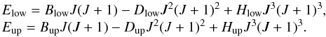
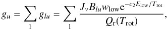
Fig. 1 Comparison of HCN content measured in the IR, among different comets. The dashed-dotted lines separate HCN depleted, HCN normal, and HCN enriched comets, while the dotted vertical line separate comets reported elsewhere (left) from those reported in this paper (right). The comets in the plot are 1. C/2004 Q2, 2. C/1999 H1, 3. C/2000 WM1, 4. C/2006 P1, 5. C/2001 A2, 6. C/1996 B2, 7. C/1995 O1, 8. C/1999 S4, 9. 1P/Halley, 10. 153P/Ikeya-Zhang, 11. 21P/Giacobini – Zinner (upper limit), 12. 73P/Schwassmann-Wachmann – Fragment C, 13. 73P Schwassmann-Wachmann – Fragment B, 14. 17P/Holmes (outburst), 15. 9P/Tempel 1 (pre impact), 16. 9P/Tempel 1 (post impact), 17. 6P/D’Arrest, 18. 8P/Tuttle, 19. C/2007 W1, 20. C/2008 Q3; (see Lippi 2010 and references therein). |
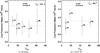 |
Fig. 2 Rotational temperature diagram for 8P/Tuttle(a) and C/2007 W1 (b). In each plot, the dashed line represents the weighted mean production rate, while the dotted line represents the “null slope” fit; individual lines are labeled with the lower level transition; error bars are plotted with vertical lines. The “null slope” rotational temperature and confidence limits are shown at top right in each panel. |
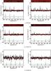 |
Fig. 3 Detection of HCN in the observed comets. For each spectrum the red line represents the ±1σ error. The model, Doppler-shifted and affected by transmittance, is plotted below the observed spectra; identified lines are indicated with a star. For comet C/2008 Q3 we omitted the echellograms, since they were too noisy to clearly distinguish the HCN emission lines. |
4.2. Production rates and mixing ratios
For each identified line, the HCN molecular production rates
Qi were retrieved through the relation
 (10)where Δ is the geocentric
distance (m), Fi (Watt/m2) is the line flux
measured in a 5 × 15 pixels box centered on the nucleus, gi is
the emission fluorescence g-factors (at heliocentric distance
Rh = 1 AU), hcν is the energy (Joules) of a
photon with wavenumber ν (cm-1), trans is the atmospheric
transmittance at the Doppler shifted frequency of the ith line at the
cometary geocentric velocity (vΔ),
f(x) is the fraction of the total coma content of the
targeted species sampled by the beam (see appendix in Hoban et al. 1991, for details), and τ is the molecular
photodissociation lifetime at heliocentric distance of 1 AU (we used a value of
6.67 × 10⁴ s, see Magee-Sauer et al.
1999, and references therein).
(10)where Δ is the geocentric
distance (m), Fi (Watt/m2) is the line flux
measured in a 5 × 15 pixels box centered on the nucleus, gi is
the emission fluorescence g-factors (at heliocentric distance
Rh = 1 AU), hcν is the energy (Joules) of a
photon with wavenumber ν (cm-1), trans is the atmospheric
transmittance at the Doppler shifted frequency of the ith line at the
cometary geocentric velocity (vΔ),
f(x) is the fraction of the total coma content of the
targeted species sampled by the beam (see appendix in Hoban et al. 1991, for details), and τ is the molecular
photodissociation lifetime at heliocentric distance of 1 AU (we used a value of
6.67 × 10⁴ s, see Magee-Sauer et al.
1999, and references therein).
Retrieved production rates Q, mixing ratios M.R., and HCN rotational temperatures Trot for the observed comets.
Since the observed beam corresponds to a small spatial coverage of the coma, the product
f(x)τ is proportional to the inverse
of the gas outflow velocity vgas; if we adopt a spherical
outflow model with vgas ∝ 0.8
 km s-1, where Rh is in AU, we can assume the
derived production rate not to be very sensitive to the assumed lifetime.
km s-1, where Rh is in AU, we can assume the
derived production rate not to be very sensitive to the assumed lifetime.
To compensate for slit-losses we calculated the growth-factor as  (11)where
Qnc is the nucleus-centered production rate, determined from
the mean of production rates derived from individual lines weighted inversely by their own
stochastic error (squared), while Qterm, is the terminal value
reached at distances beyond the slit-loss region, computed by taking the mean value of
production rates extracted at positions equidistant from the nucleus, along the spatial
profile (see Xie & Mumma 1996; Dello Russo et al. 1998; Bonev 2005).
(11)where
Qnc is the nucleus-centered production rate, determined from
the mean of production rates derived from individual lines weighted inversely by their own
stochastic error (squared), while Qterm, is the terminal value
reached at distances beyond the slit-loss region, computed by taking the mean value of
production rates extracted at positions equidistant from the nucleus, along the spatial
profile (see Xie & Mumma 1996; Dello Russo et al. 1998; Bonev 2005).
HCN emission lines were identified in the measured spectra at their expected Doppler-shifted positions (Table 5, rest-line frequencies were calculated using the method described in 2.2). HCN production rates, mixing ratios relative to water (in percent) and rotational temperatures obtained from these data are listed in Table 3; in the same table H2O production rates (needed to retrieve HCN/H2O mixing ratios) are indicated, with the respective references.
For 8P, the HCN setting spanned 3345.39 to 3259.90 cm-1, allowing us to sample eleven emission lines (see Table 5); in our analysis, we only considered lines that were not blended with emissions from other species. We retrieved a production rate of (0.28 ± 0.03) × 1026 mol/s, and a mixing ratio (relative to water) of (0.05 ± 0.01)% (Böhnhardt et al. 2008 presented our results for H2O and other molecules observed on this night). Our mixing ratio for HCN on UT 27 January 2008 agrees (within 1σ confidence limits) with values obtained on the following night (0.07 ± 0.02) with CRIRES (UT 28 January 2008, Kobayashi et al. 2010), and on UT 22–23 December 2007 using NIRSPEC (0.07 ± 0.01, Bonev et al. 2008).
In comet C/2007 W1, we detected ten emission lines in the spectral region 3332.64–3263.98 cm-1 (see Table 5) and retrieved a production rate of (0.38 ± 0.02) × 1026 mol/s, which corresponds to a mixing ratio relative to water of (0.39 ± 0.02)%. This value is lower than that (0.50 ± 0.01)% presented in Villanueva et al. (2011a). However, these authors suggested a correction of the mixing ratio for apolar species due to the possible existence of an extended source of water: in this case the HCN content would be lower, which would bring it more in line with our measurement.
HCN in comet C/2008 Q3 was measured on June 8, 2009, and even though the data were noisier than the other two datasets, we were able to identify seven emission lines between 3344.10 and 3273.98 cm-1 (see Table 5) and to retrieve a production rate of (0.69 ± 0.08) × 1026 mol/s, which translates into a mixing ratio relative to water of (0.30 ± 0.03)%.
Comparing the abundance ratios (HCN/H2O) measured among different comets (see Table 4 and Fig. 1), we note that HCN (0.05%) in 8P is much lower than in the other comets, except for 6P/d’Arrest (0.03%). By contrast, the HCN content in C/2007 W1 (0.39%) is comparable to that of comet C/1995 O1 (0.40%), while comet C/2008 Q3 shows 0.30%, similar to that of 73P Schwassmann-Wachmann 3 – Fragment B. In terms of the classification in Mumma et al. (2003) and DiSanti & Mumma (2008), we conclude that C/2007 W1 is HCN-enriched, while 8P is depleted in this species.
Comparison with other comets.
4.3. Spatial profiles
The spatial profiles for molecular or continuum emissions along the slit can be used to determine the origin and outgassing of material in cometary comae. If volatiles are released solely and uniformly from the nucleus and flow outward with constant velocity, their intensity distribution along the spatial direction is expected to scale as 1/ρ, with ρ being the projected distance from the nucleus. For species that are emitted from small ice grains in the coma (distributed sources) the intensity will instead fall off more slowly than 1/ρ. However, it is important to notice that other properties of the comet (e.g., outflow asymmetries) and observing conditions (primarily seeing and tracking errors) may cause a deviation from the 1/ρ dependence, even in the absence of a distributed source.
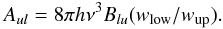
We obtained the spatial profile for 8P and C/2007 W1 by co-adding the single-line spatial profiles observed in our spectra; the results are shown in Fig. 4; for comet C/2008 Q3 the number of the useful (bright and not blended) lines was too small to retrieve a good spatial profile.
The two comets present symmetric profiles that scale approximately like 1/ρ. Comet 8P shows a small excess in the solar direction, which can be interpreted as a higher activity of the comet on the day-side with respect to the night-side. In contrast, the C/2007 W1 profile shows an excess in the anti-solar direction that could be interpreted as an indication of localized enhanced activity either coming as HCN directly from the nucleus (jets), or produced by dust grains or icy grains coming from the nucleus. C/2007 W1 was also observed in July 2008 by Villanueva et al. (2011a), displaying spatial profiles that are symmetric for HCN (and C2H6), and quite asymmetric for polar molecules (e.g., H2O and CH3OH). These asymmetries are much more pronounced than the one we saw for HCN in May 2008, and it is possible that the small asymmetry we detected is more related to the dissimilar conditions during the two observations (pre-/post perihelion, geo and heliocentric distances, integrating field of views, etc.) than to an effective HCN activity on the comet.
Since for 8P/Tuttle the dust signal was particularly strong, it was possible to compare the spatial profile of dust with that of HCN (Fig. 4a); the dust profile is also symmetric and shows a 1/ρ dependence.
4.4. HCN and CN production rates
Although CN has been easily observed in the visible spectral range since the earliest days of cometary spectroscopy, its origin is still only poorly understood. One of the candidate primary molecules is HCN, but direct comparisons show an inconsistency for this hypothesis; in these cases CN is thought to come partially from the dust grains present in the coma (Fray et al. 2005).
For comet 8P/Tuttle the CN radical was measured in the beginning of Dec. 2007 by Schleicher using narrow-band photometry (Schleicher & Woodney 2007); at which time, the comet was 1.30 AU from the Sun. The reported production rates for CN (≈1.66 × 1025 mol/s) and OH (≈759 × 1025 mol/s) imply a mixing ratio CN/OH of 0.22% in this comet. Thus, our derived mixing ratio for HCN in 8P (0.05 ± 0.01%) is too low to support HCN as the only parent of the CN radical; this agree with the result presented in Jehin et al. (2009), who provided simultaneous observations of HCN and CN, and with both Bonev et al. (2008) and Kobayashi et al. (2010), who made similar comparisons and reached the same conclusion.
Narrow-band photometry of comet C/2007 W1, observed on 30–31 July 2008, give the following results: OH production rate ≈6.16 × 1027 mol/s, CN production rate ≈2.34 × 1025, C2 production rate ≈4.04 × 1025 (Schleicher 2008). In that period the comet was at 1.07 AU from the Sun. If we scale our retrieved production rate for HCN (0.38 × 1026 mol/s, for rh = 0.97 AU), we obtain a production rate of ≈(3.1 ± 0.3) × 1025 mol/s; unlike in the case of 8P/Tuttle, this result would be consistent with HCN being the only primary species of CN.
Identified HCN emission lines for the three comets.
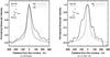 |
Fig. 4 Spatial profiles for 8P/Tuttle(a) and C/2007 W1 (b). In each plot, the HCN profile (continuum line) is compared with a 1/ρ profile (dash-dotted line). The direction of the Sun is also indicated. |
Regarding comet C/2008 Q3, no measurements for CN have been found in the literature.
The different correlation that we found for HCN and CN in comets 8P and C/2007 W1 may depend on different compositional properties of comets and/or on different processes that can be present in the coma. In particular, these two comets have shown a different behavior regarding dust production rates: comet 8P showed in our spectra a higher dust continuum signal than did comet C/2007 W1: it is then possible that, for comet C/2007 W1, CN was produced only from photolysis of HCN, while in comet 8P/Tuttle this radical was also released from dust grains in the coma.
5. Summary and conclusions
Comets are believed to be the remnants of solar system formation and as such they can provide unique information regarding the chemical and physical conditions in the region where they formed. High-resolution spectroscopy is fundamental for retrieving the volatile composition of cometary nuclei and for testing their nature and role in the solar system; in this scenario, HCN is a cometary primary molecule that plays an important role, since it is considered a candidate for the development of life on Earth.
We reported HCN production rates, mixing ratios relative to water (in percent), and rotational temperatures that we retrieved for three comets: 8P/Tuttle, C/2007 W1 (Boattini), and C/2008 Q3 (Garradd). To that end, we developed a new fluorescence model for ν1 of HCN, which calculates fluorescence efficiencies using the latest spectroscopic parameters and includes several effects (torsional Coriolis interactions, torsional splittings, Herman-Wallis effects, resonance mixing, etc.) that are often excluded in the computation of cometary g-factors; moreover, our calculation corrects the g-factors for the Swings effect and uses a more realistic solar spectrum, obtained by combining empirical and theoretical data.
The observed comets displayed considerable differences, with comet 8P (a Halley-type comet) containing a very low abundance of HCN with respect to comets C/2007 W1 and C/2008 Q3, both classified as dynamically new comets. As shown in Table 4, Oort Cloud comets appear to show higher HCN abundances than Halley-type and Jupiter-family comets; in this limited sample of comets, the enrichment of HCN observed in comets C/2007 W1 and C/2008 Q3 and its depletion in 8P is consistent with this grouping.
We analyzed the spatial intensity distribution of HCN for comet 8P and C/2007 W1, finding quite symmetric profiles, suggesting that HCN is released at (or very close to) the nucleus for all these comets.
Finally, for comets 8P and C/2007 W1, we compared production rates of the primary molecule HCN with the product species CN to check a possible correlation between them: while in comet C/2007 W1 the mixing ratios of the two molecules are comparable, in 8P the abundance of HCN is not sufficient to explain the CN production in the comet, and more investigations are needed to find other possible primary candidates for this molecule.
See Nakano notes NK 1656 and NK 1886 at http://www.oaa.gr.jp/~oaacs/nk.htm
Acknowledgments
We thank the VLT science operations team of the European Southern Observatory for efficient execution of the observations. This work was supported by the International Max Planck Research School, NASA’s Planetary Astronomy Program, Astrobiology Program and Postdoctoral Program and the German-Israeli Foundation for Scientific Research and Development.
References
- Böhnhardt, H., Mumma, M. J., Villanueva, G. L., et al. 2008, ApJ, 683, L71 [NASA ADS] [CrossRef] [Google Scholar]
- Bonev, B. P. 2005, Ph.D. Thesis, The University of Toledo [Google Scholar]
- Bonev, B. P., Mumma, M. J., Radeva, Y. L., et al. 2008, ApJ, 680, L61 [NASA ADS] [CrossRef] [Google Scholar]
- Bonev, B. P., Villanueva, G. L., Paganini, L., et al. 2013, Icarus, 222, 740 [NASA ADS] [CrossRef] [Google Scholar]
- Clough, S. A., Shephard, M. W., Mlawer, E. J., et al. 2005, J. Quant. Spectr. Radiat. Transf., 91, 233 [Google Scholar]
- Crovisier, J. 1987, A&A, 68, 223 [Google Scholar]
- Dello Russo, N., DiSanti, M. A., Mumma, M. J., Magee-Sauer, K., & Rettig, T. W. 1998, Icarus, 135, 377 [NASA ADS] [CrossRef] [Google Scholar]
- Dello Russo, N., DiSanti, M. A., Magee-Sauer, K., et al. 2004, Icarus, 168, 186 [NASA ADS] [CrossRef] [Google Scholar]
- DiSanti, M. A., & Mumma, M. J. 2008, Space Sci. Rev., 138, 127 [NASA ADS] [CrossRef] [Google Scholar]
- DiSanti, M. A., Mumma, M. J., Dello Russo, N., & Magee-Sauer, K. 2001, Icarus, 153, 361 [NASA ADS] [CrossRef] [Google Scholar]
- DiSanti, M. A., Bonev, B. P., Magee-Sauer, K., et al. 2006, ApJ, 650, 470 [NASA ADS] [CrossRef] [Google Scholar]
- Fray, N., Bénilan, Y., Cottin, H., Gazeau, M.-C., & Crovisier, J. 2005, Planet. Space Sci., 53, 1243 [NASA ADS] [CrossRef] [Google Scholar]
- Hartogh, P., Crovisier, J., de Val-Borro, M., et al. 2010, A&A, 518, L150 [NASA ADS] [CrossRef] [EDP Sciences] [Google Scholar]
- Hase, F., Demoulin, P., Sauval, A., et al. 2006, J. Quant. Spectr. Radiat. Transf., 102, 450 [NASA ADS] [CrossRef] [Google Scholar]
- Hoban, S., Mumma, M., Reuter, D. C., et al. 1991, Icarus, 93, 122 [NASA ADS] [CrossRef] [Google Scholar]
- Jehin, E., Bockelée-Morvan, D., Dello Russo, N., et al. 2009, Earth Moon and Planets, 105, 343 [CrossRef] [Google Scholar]
- Käufl, H., Ballester, P., Biereichel, P., et al. 2004, in SPIE Conf. Ser. 5492, eds. A. F. M. Moorwood, & M. Iye, 1218 [Google Scholar]
- Kobayashi, H., Bockelée-Morvan, D., Kawakita, H., et al. 2010, A&A, 509, A80 [NASA ADS] [CrossRef] [EDP Sciences] [Google Scholar]
- Kurucz, R. L. 1997, in IAU Symp. 189, eds. T. R. Bedding, A. J. Booth, & J. Davis, 217 [Google Scholar]
- Lippi. 2010, Ph.D. Thesis, Technische Universität Braunschweig, Germany (UNI-Ed.) [Google Scholar]
- Magee-Sauer, K., Mumma, M. J., DiSanti, M. A., Russo, N. D., & Rettig, T. W. 1999, Icarus, 142, 498 [NASA ADS] [CrossRef] [Google Scholar]
- Maki, A., Quapp, W., Klee, S., Mellau, G. C., & Sieghard, A. 1996, J. Mol. Spectrosc., 180, 323 [NASA ADS] [CrossRef] [PubMed] [Google Scholar]
- Malathy Devi, V., Benner, D., Smith, M., et al. 2003, JQSRT, 82, 319 [NASA ADS] [CrossRef] [Google Scholar]
- Matthews, C. N., & Minard, R. D. 2008, in IAU Symp. 251, eds. S. Kwok, & S. Sandford, 453 [Google Scholar]
- Mumma, M. J., & Charnley, S. B. 2011, ARA&A, 49, 471 [NASA ADS] [CrossRef] [Google Scholar]
- Mumma, M. J., Weissman, P. R., & Stern, S. A. 1993, in Protostars and Planets III, eds. E. H. Levy, & J. I. Lunine, 1177 [Google Scholar]
- Mumma, M. J., McLean, I. S., DiSanti, M. A., et al. 2001, ApJ, 546, 1183 [NASA ADS] [CrossRef] [Google Scholar]
- Mumma, M. J., DiSanti, M. A., Dello Russo, N., et al. 2003, Adv. Space Res., 31, 2563 [NASA ADS] [CrossRef] [Google Scholar]
- Rothman, L. S., Gordon, I. E., Barbe, A., et al. 2009, J. Quant. Spectr. Radiat. Transf., 110, 533 [Google Scholar]
- Schleicher, D. 2008, IAU Circ., 7342, 1 [Google Scholar]
- Schleicher, D., & Woodney, L. 2007, IAU Circ., 8903, 1 [NASA ADS] [Google Scholar]
- Šimečková, M., Jacquemart, D., Rothman, L. S., Gamache, R. R., & Goldman, A. 2006, J. Quant. Spectr. Radiat. Transf., 98, 130 [CrossRef] [Google Scholar]
- Swings, P. 1941, Lick Obs. Bull., 19, 131 [NASA ADS] [CrossRef] [Google Scholar]
- Villanueva, G. L., Mumma, M. J., Novak, R. E., & Hewagama, T. 2008, Icarus, 195, 34 [NASA ADS] [CrossRef] [Google Scholar]
- Villanueva, G. L., Mumma, M. J., DiSanti, M. A., et al. 2011a, Icarus, 216, 227 [NASA ADS] [CrossRef] [Google Scholar]
- Villanueva, G. L., Mumma, M. J., & Magee-Sauer, K. 2011b, J. Geophys. Res. Pl., 116, E08012 [NASA ADS] [CrossRef] [Google Scholar]
- Xie, X., & Mumma, M. J. 1992, ApJ, 386, 720 [NASA ADS] [CrossRef] [Google Scholar]
- Xie, X., & Mumma, M. J. 1996, ApJ, 464, 442 [NASA ADS] [CrossRef] [Google Scholar]
All Tables
Retrieved production rates Q, mixing ratios M.R., and HCN rotational temperatures Trot for the observed comets.
All Figures
|
Fig. 1 Comparison of HCN content measured in the IR, among different comets. The dashed-dotted lines separate HCN depleted, HCN normal, and HCN enriched comets, while the dotted vertical line separate comets reported elsewhere (left) from those reported in this paper (right). The comets in the plot are 1. C/2004 Q2, 2. C/1999 H1, 3. C/2000 WM1, 4. C/2006 P1, 5. C/2001 A2, 6. C/1996 B2, 7. C/1995 O1, 8. C/1999 S4, 9. 1P/Halley, 10. 153P/Ikeya-Zhang, 11. 21P/Giacobini – Zinner (upper limit), 12. 73P/Schwassmann-Wachmann – Fragment C, 13. 73P Schwassmann-Wachmann – Fragment B, 14. 17P/Holmes (outburst), 15. 9P/Tempel 1 (pre impact), 16. 9P/Tempel 1 (post impact), 17. 6P/D’Arrest, 18. 8P/Tuttle, 19. C/2007 W1, 20. C/2008 Q3; (see Lippi 2010 and references therein). |
| In the text | |
|
Fig. 2 Rotational temperature diagram for 8P/Tuttle(a) and C/2007 W1 (b). In each plot, the dashed line represents the weighted mean production rate, while the dotted line represents the “null slope” fit; individual lines are labeled with the lower level transition; error bars are plotted with vertical lines. The “null slope” rotational temperature and confidence limits are shown at top right in each panel. |
| In the text | |
|
Fig. 3 Detection of HCN in the observed comets. For each spectrum the red line represents the ±1σ error. The model, Doppler-shifted and affected by transmittance, is plotted below the observed spectra; identified lines are indicated with a star. For comet C/2008 Q3 we omitted the echellograms, since they were too noisy to clearly distinguish the HCN emission lines. |
| In the text | |
|
Fig. 4 Spatial profiles for 8P/Tuttle(a) and C/2007 W1 (b). In each plot, the HCN profile (continuum line) is compared with a 1/ρ profile (dash-dotted line). The direction of the Sun is also indicated. |
| In the text | |
Current usage metrics show cumulative count of Article Views (full-text article views including HTML views, PDF and ePub downloads, according to the available data) and Abstracts Views on Vision4Press platform.
Data correspond to usage on the plateform after 2015. The current usage metrics is available 48-96 hours after online publication and is updated daily on week days.
Initial download of the metrics may take a while.