| Issue |
A&A
Volume 551, March 2013
|
|
|---|---|---|
| Article Number | A110 | |
| Number of page(s) | 17 | |
| Section | Interstellar and circumstellar matter | |
| DOI | https://doi.org/10.1051/0004-6361/201219517 | |
| Published online | 04 March 2013 | |
Deep optical imaging of asymptotic giant branch circumstellar envelopes⋆,⋆⋆
1
Laboratoire Univers et Particules de Montpellier, UMR 5299 CNRS
& Université de Montpellier II,
Case CC72, Place Bataillon,
34095
Montpellier Cedex 5,
France
e-mail: nicolas.mauron@univ-montp2.fr
2
Physics Department, New York University,
4 Washington Place,
NY
10003
New York,
USA
Received: 2 May 2012
Accepted: 18 December 2012
We report results of a program to image the extended circumstellar envelopes of asymptotic giant branch (AGB) stars in dust-scattered Galactic light. The goal is to characterize the shapes of the envelopes to probe the mass-loss geometry and the presence of hidden binary companions. The observations consist of deep optical imaging of 22 AGB stars with high mass loss rates: 16 with the ESO 3.6 m NTT telescope, and the remainder with other telescopes. The circumstellar envelopes are detected in 15 objects, with mass loss rates ≳2 × 10⁻⁶ M⊙ yr-1. The surface brightness of the envelopes shows a strong decrease with Galactic radius, which indicates a steep radial gradient in the interstellar radiation field. The envelopes range from circular to elliptical in shape, and we characterize them by the ellipticity (E = major/minor axis) of iso-intensity contours. We find that ~50% of the envelopes are close to circular with E ≲ 1.1, and others are more elliptical with ~20% with E ≳ 1.2. We interpret the shapes in terms of populations of single stars and binaries whose envelopes are flattened by a companion. The distribution of E is qualitatively consistent with expectations based on population synthesis models of binary AGB stars. We also find that ~50% of the sample exhibit small-scale, elongated features in the central regions. We interpret these as the escape of light from the central star through polar holes, which are also likely produced by companions. Our observations of envelope flattening and polar holes point to a hidden population of binary companions within the circumstellar envelopes of AGB stars. These companions are expected to play an important role in the transition to post-AGB stars and the formation of planetary nebulae.
Key words: stars: AGB and post-AGB / stars: mass-loss / circumstellar matter
Based on observations made at the European Southern Observatory, Chile (programs 078.D-0102, 082.D-0338 and 0.84.D-0302) and on de-archived data obtained with the ESO Very Large Telescope and with the NASA/ESA Hubble Space Telescope.
Appendix A and Figs. 5, 6 are available in electronic form at http://www.aanda.org
© ESO, 2013
1. Introduction
It is well established that stars lose a significant fraction of their mass during evolution on the asymptotic giant branch (AGB). The mass loss forms expanding envelopes of molecular gas and dust around the stars, and eventually recycles the stellar material back into the interstellar medium (ISM). The circumstellar envelopes are important for the study of many astrophysical processes, including circumstellar chemistry and dust formation. They are also important for stellar and galactic evolution, especially in connection with the formation of planetary nebulae. For reviews on AGB envelopes and their properties see, e.g., Habing & Olofsson (2004) and Kerschbaum et al. (2011).
Properties of the AGB stars.
Despite extensive study, there are many aspects of AGB envelopes that are not well understood. Here we focus on one of the most basic properties, the geometry of the envelopes. On large size scales the morphology is known to be affected by interaction with the ISM (e.g. Cox et al. 2012), but the shaping mechanisms close to the star are not well understood. It is not known if the mass loss of single stars is closely spherically symmetric, or if it is influenced by factors such as the stellar magnetic field. Binary companions are expected to influence the geometry, but information on the presence of companions is problematic. Apart from symbiotic systems, only a few dozen AGB binaries are known (Jorissen 2008), even though they are expected to be common. The reason so few are detected is because of the luminosity and variability of the AGB stars, and the opacity of their circumstellar envelopes. There must be a large population of hidden companions that can interact with the envelopes.
The effects that stellar companions can have on AGB envelopes is suggested by hydrodynamical simulations (Theuns & Jorissen 1993; Mastrodemos & Morris 1999; Gawryszczak 2002). There are two main interactions. First, the reflex motion of the AGB star forms a spiral pattern in the envelope, and this has been detected in the case of AFGL 3068 (Mauron & Huggins 2006, hereafter MH06; Morris et al. 2006). Second, the large scale geometry of the envelope is expected to be flattened by a companion, and this has been discussed by Huggins et al. (2009) as a possible probe of the presence of binary companions. Indirect shaping effects on the envelopes by jets launched from accretions disks around a companion are also possible, as seen in the case of Mira (Josselin et al. 2000).
There is a lack of detailed observational information on the structure of circumstellar envelopes because the relatively cool material in the envelopes is difficult to image at high resolution. A review of techniques is given by Marengo (2009). Recent advances include millimeter interferometry of the molecular gas (e.g., Castro-Carrizo et al. 2010) and imaging of the thermal dust emission, in the mid-infrared with ground-based observations (e.g., Lagadec et al. 2011) and in the far infrared with Herschel (Decin et al. 2011). In this paper, we report progress using a different technique: observing the envelopes in dust-scattered Galactic light. This technique makes use of deep optical imaging, so that high resolution is more readily attained than at longer wavelengths.
Our initial observations using deep optical imaging produced the first wide field image of the circumstellar envelope of the AGB archetype IRC+10216 at arcsecond resolution (Mauron & Huggins 1999, 2000). The core of the envelope is illuminated by light from the central star, but the extended envelope is illuminated by the ambient Galactic radiation field, which reveals the detailed structure. We subsequently carried out pilot observations of other, more distant AGB stars, and found that the technique can provide useful information on the shapes of the circumstellar envelopes (MH06). In this paper, we report more extensive observations using the New Technology Telescope (NTT) at the European Southern Observatory at La Silla (Chile), with arcsecond resolution and exposures up to several hours. The goal is to extend the sample of AGB stars with resolved envelopes to determine their geometry.
Section 2 describes the observations; Sect. 3 presents the images and information on the shapes, together with those of our earlier observations in the same format; and Sect. 4 discusses the results and their implications.
2. Observations
2.1. The sample
The deep imaging technique is well suited for investigating the shapes of the circumstellar envelopes of AGB stars with high mass loss rates. The thickest envelopes produce the maximum surface brightness and the largest envelope sizes for observation in dust scattered Galactic radiation. The high opacity of these envelopes also reduces or eliminates the stellar light contribution, which may be affected by structure close to the star and can mask the faint, external illumination.
The AGB targets for observations were selected from the catalog of Loup et al. (1993), on the basis of strong IRAS fluxes and large infrared excesses (small f12/f25 ratios), as well as declinations accessible from La Silla. Preference was given to stars at relatively high galactic latitude, in order to minimize the effects of interstellar extinction and crowded star fields.
Details of all the AGB stars discussed in the paper are given in Table 1. The list includes new targets observed with the NTT (Sect. 2.2) and earlier observations which we include for completeness (Sect. 2.3). Table 1 gives the name, the Galactic co-ordinates, the chemistry (oxygen-rich or carbon-rich), distance d, expansion velocity Vexp, mass-loss rate Ṁ, and relevant IRAS fluxes from the point source catalog. It can be seen that they represent AGB stars in the solar neighborhood (within a few kpc) with high mass loss rates, comparable in many cases with IRC+10216.
Details of NTT observations.
2.2. NTT observations
The observations with the NTT were carried out in four observing runs. Two were made with the EMMI instrument in imaging mode on 12–14 October 2006 and 16–18 March 2007, and two were made with the EFOSC2 instrument on 20−23 February 2009 and 15–19 October 2009. The angular field is  with a pixel size of
  for EMMI, and
  with a pixel size of
  for EFOSC2. The first two observing runs were affected by poor weather, so most of the data reported are with EFOSC2, which also has greater sensitivity and better sampling of the PSF.
Details of the observations including the instrument, the filters, and the exposure times are listed in Table 2. In many cases, we first secured an I-band exposure to ascertain the precise position of the target. The deep B or V images to detect the faint envelopes were made with a series of individual exposures, typically of 30 min each, with a small shift in α or δ between them to improve the quality of the final image. The data were reduced using standard procedures with the MIDAS software: bias subtraction, flat-fielding with flats made on the dome or the sky, and the removal of cosmic-rays hits. The individual frames were then shifted and stacked. In some cases, we corrected residual gradients in the background level using division by a normalized polynomial of order 1 or 2.
The photometric calibration of the EFOSC2 observations was made using photometric sequences close to the star T Phe and in the field SA 98-642 (Snodgrass 2009). For these observations, the relation between magnitudes and ADU counts is found to be:

 for the V-band, where X is the air-mass, and t is the exposure in seconds. For each relation, B or V is the stellar magnitude if F is the spatially integrated ADU count for the star, or the surface brightness if F is the ADU count per arcsec2 measured on an extended object. The coefficients of X are the usual extinction coefficients for photometric nights at La Silla: the quoted values are from the documentation of the 1.54 Danish telescope. Overall the calibrations are expected to have an uncertainty of 0.1 mag, and the results are found to be consistent within 0.05 mag when comparing the two EFOSC2 runs.
Observations from earlier work.
The photometric calibration for the EMMI observations was made by considering un-saturated stars and their B-band magnitudes taken from the USNO-B1.0 catalog (Monet et al. 2003); in this case the photometric uncertainty is ~0.4 mag (1-σ). Comparisons of the calibration with the USNO catalog and the EFOSC2 photometric calibration are consistent with this.
The envelopes illuminated by the ambient Galactic radiation field are faint, typically a few percent of the sky background. Hence the limiting factor for envelope detection is the sky noise. The exposures reported here are relatively long, and all the runs were made in dark time. The results are therefore representative of the quality of the data that can be obtained with this technique, using an intermediate sized, ground-based telescope.
2.3. Additional observations
For completeness, we include in the analysis the observations from our earlier report (MH06) which are of comparable quality to the NTT data. These observations are summarized in Table 3, and have been processed in the same way.
The observations include short exposures with the Very Large Telescope (VLT), longer exposures with the 1.54 m ESO Danish Telescope (DT) and the 1.20 m telescope of the Observatoire de Haute-Provence (OHP), and archival images made with the HST. The VLT-FORS raw images and calibration files were extracted from the ESO archive. The V-band image of IRC+10216 was first shown by Leao et al. (2006). The HST data are from programs 9463 and 10185, PI: R. Sahai. Further details of the observations are given in MH06. Observations in MH06 but not in Table 3 include several non-detections which are much poorer than the NTT data, and AFGL 3068. In AFGL 3068, the illumination is highly directional and the envelope shows a strong spiral pattern, which both limit the ability to measure the overall shape.
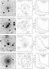 |
Fig. 1 Images and radial profiles of the AGB envelopes. Each row shows from left to right: the image in grayscale; a close-up contour map of the envelope, with field stars removed and their cores masked; and the radial profile of the envelope with the PSF. The field size is indicated in the images. The filters and contours, specified by the lowest contour (and contour interval) in units of the peak surface brightness of the envelope, are as follows (from top to bottom): IRAS 01037+1219, V-band, contours 0.33 (0.43); IRAS 07454−7112, B-band, contours 0.31 (0.23); IRAS 09116−2439, B-band, contours 0.28 (0.26); IRAS 09452+1330, V-band, contours 0.32 (0.16). The images are square, with north to the top and east to the left. |
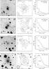 |
Fig. 2 Continuation of Fig. 1. From top to bottom: IRAS 10323−4611, B-band, contours 0.13 (0.25); IRAS 12384−4536, V-band, contours 0.25 (0.25); IRAS 14591−4438, B-band, contours 0.35 (0.33); IRAS 16029−3041, V-band, contours 0.17 (0.17). The images are square, with north to the top and east to the left. |
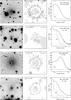 |
Fig. 3 Continuation of Fig. 1. From top to bottom: IRAS 17319−6234, V-band, contours 0.12 (0.19); IRAS 18240+2326, V-band, contours 0.34 (0.23); IRAS 18467−4802, F606W (HST/ACS), contours 0.27 (0.25); IRAS 19178−2620, B-band, contours 0.18 (0.22). The images are square, with north to the top and east to the left. |
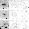 |
Fig. 4 Continuation of Fig. 1. From top to bottom: IRAS 20077−0625, V-band, contours 0.20 (0.18); IRAS 23257+1038, V-band, contours 0.20 (0.31); IRAS 23320+4316, B-band, contours 0.29 (0.29). The images are square, with north to the top and east to the left. |
3. The images
3.1. Presentation of the images
The main results of the observations are summarized in Table 4. Column (2) gives the telescope used for the V and B observations, and Col. (3) indicates the detection of the envelope and/or the central star (or the star-illuminated core) at these wavebands. For the NTT observations, seven of the envelopes are not detected and are discussed in the appendix.
Figures 1–4 present observations of each detected envelope, in three panels: a gray-scale image of the field in the waveband that best shows the envelope shape, a close-up contour map of the envelope, and the azimuthally averaged, radial intensity profile.
Observations of the circumstellar envelopes.
In many of the gray-scale images it can be seen that field stars and galaxies lie along the lines of sight to the envelopes. To make the contour maps, the images are cleaned by removing these features using the following procedures. For bright stars whose halos extend over part of the envelope, we fit and subtract circularly symmetric halo models. The models are derived from isolated field stars in the same image, and the fit is made by minimizing residuals in regions outside the envelope. The cores of these bright stars are also masked. In the case of IRAS 07454−7112, a relatively bright elliptical galaxy lies close to the AGB star to the south-east, and this was successfully subtracted using a Sersic galaxy profile (Sersic 1963). Dimmer stars and small galaxies, are simply masked. All masked areas are then replaced with local averages. This local average is determined by considering sectors centered on the AGB star with radial widths of 1–2′′, and typical ranges in position angle of ± 20−30°. In this way, the masked areas are filled with representative local intensities, and Gaussian noise similar to the sky noise is added in these areas.
For the contour maps in Figs. 1–4, the cleaned images were lightly smoothed with a Gaussian of width 2 pixels (FWHM) with two exceptions noted in Sect. 3.5. The gray areas in the figures show the masked regions as described above. The solid contours are linearly spaced, and are specified in the figure captions in units of the peak surface brightness of the envelopes; the equivalent values in mag arcsec-2 are given in Table 4. In cases with a strong stellar core, additional dashed contours are included with a step size equal to the level of the highest solid contour. In Figs. 5 and 6, the cleaned images are shown in color, with the contours superposed.
3.2. General properties
As described in MH06, deep optical imaging of AGB stars may reveal one or more of the following: the central star or an unresolved stellar core; the star-illuminated inner envelope; and the extended envelope illuminated by the ambient Galactic radiation field. The typical situation for the thick circumstellar envelopes is that the star and the star-illuminated core are faint (or not seen) in the B or V bands (because of extinction by the envelope), but the star becomes dominant at longer wavelengths because of the decreasing opacity of the dust envelope and the red spectrum of the star.
For the star-illuminated inner envelope, the intensity of scattered starlight decreases rapidly with angular distance from the center (~θ-3, Martin & Rogers 1987). For external illumination, a faint, extended nebula is seen, with a shallow radial dependence. The externally illuminated nebula may also form a plateau of relatively constant intensity in the central regions where the optical depth to external radiation is ≳1. Examples of this (e.g., IRAS 16029−3041) may be seen in the radial profiles in Figs. 1–4.
3.3. Surface brightness
Column (4) of Table 4 lists the peak surface brightness in B or V for each circumstellar envelope, based on the photometry described in Sect. 2.2 and MH06. For cases where the envelope is detected and the star is of low intensity or not detected, or the envelope plateau is extended, the measurement is straightforward. For cases where the envelope is detected, but the central star is of high intensity, we estimate the peak intensity by fitting and removing the stellar contribution at the center by using the profiles of field stars. For cases where neither the envelope nor the star is detected, we give upper limits assuming the source size is comparable to the seeing disk (FWHM). For cases where the star (or stellar core) is detected but not the envelope, a small source is essentially invisible; for these we give nominal limits based on the smallest source that would be detectable: 3″ for IRAS 06255−4928 and 09521−7508 and 5″ for IRAS 05418−3224 and 20042−4241.
For three envelopes we are able to measure both the B and V surface brightness. In addition to the B values given in Table 4, V = 25.04 mag arcsec-2 for the C-rich envelope IRAS 09452+1330, and V = 23.43 and 23.07 mag arcsec-2, for the O-rich envelopes IRAS 16029−3041 and 17319−6234, respectively.
In addition to the measured values, Table 4 also lists an effective surface brightness in the B-band, B0, corrected for interstellar extinction, and where necessary, transformed from V-band measurements. The extinction used is from the NED1 calculator, assuming all extinction along each line of sight lies between us and the star. For envelopes with only V-band measurements, we first correct for extinction, and then adopt the extinction corrected color (B − V)0 appropriate to the chemistry of the envelope. The colors are obtained from the three envelopes measured in both bands given above. For the C-rich envelope, (B − V)0 = 0.72 mag, and for the mean of the O-rich envelopes, (B − V)0 = 0.99 mag. Thus the two types of envelopes are fairly similar.
3.4. Envelope shapes
Inspection of the images in Figs. 1–6 shows that the envelopes exhibit relatively smooth and symmetric shapes that reveal their large scale geometry. They range from close to circular to distinctly elliptical.
There are two additional features. First, three envelopes show elongated central components. These we interpret as the result of the leakage of light from the central star through polar (or bipolar) openings in the core of the envelope, as is the case in IRC+10216 (Mauron & Huggins 2000). Several additional cases are seen on smaller scales in HST images of the sample (MH06; Sahai 2007). The polar cores are noted in Table 4, and details are given in Sect. 3.5.
A second feature of the envelopes of IRAS 16029−3041, 17319−6234 and 18467−4802 is a one-sided asymmetry in the optically thick central region, which results from asymmetry in the external illumination. This is most clearly seen as a crescent shape in the highest level contours. In all three cases the direction of maximum illumination indicated by the crescent is within 30° of the direction of the Galactic plane. The asymmetry is reduced in the outer, optically thin regions of the envelopes where the observed intensity is less sensitive to the directionality of the illumination.
To quantify the overall shapes of the envelopes, we fit ellipses to intensity contours at specified levels. Our procedure samples an intensity contour at intervals of 10° in position angle, omitting regions masked by the presence of field stars, as described in Sect. 3.1. An ellipse is then fit to the data using a non-linear least squares model, with the lengths of the semi-major and semi-minor axes (a and b), the center of the ellipse, and the position angle (PA) of the major axis as parameters of the fit. The shape is then given by the ellipticity E, where E = a/b.
An example of the results of this procedure for the case of IRAS 17319−6234 is shown in Fig. 7. The figure shows data points sampled at levels of 20% and 40% of the envelope peak intensity, and the fitted ellipses for which values of E are 1.05 ± 0.02 and 1.09 ± 0.03, respectively. In spite of gaps in the data because of the masking of field stars in the image, the shapes are well constrained by the procedure. In this case the envelope is marginally non-circular, probably on account of asymmetric illumination seen in the plateau in the image in Fig. 5.
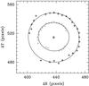 |
Fig. 7 Contour fitting for IRAS 17319−6234. The inner (gray) and outer (black) crosses sample the envelope at 10° intervals in azimuth and at 20% and 40% of the peak intensity, respectively. Gaps in the data correspond to masked regions of the image. The curves show the fitted ellipses; the small inner circles show the fitted centers. |
Using this technique, we characterize the shapes of the envelopes on the largest size scales allowed by the observations in order to minimize the effects of contamination by the central star (when visible) and the core features noted above. The results are given in Table 4. For cases with good signal-to-noise ratio (S/N) and resolved plateaus, we give the shape measured at 20% of the peak. For the other envelopes, which are fainter and less well defined at this level, we give the shape at the 40% of the peak; Table 4 lists the fitted values of E (± 1σ), a, and the PA of the major axis. The expansion time scale, texp corresponding to a is also given, based on the distances and expansion velocities given in Table 1. The envelopes are detected to significantly larger radii in the azimuthally averaged profiles, as seen in Figs. 1–4.
The envelope shapes and orientations at higher intensity levels are generally similar to those in Table 4. However there are several exceptions where the inner ellipticity is larger and at a different PA, especially in cases which have the core features noted above. Individual cases are discussed below.
3.5. Notes on individual objects
IRAS 01037+1219 (IRC+10011). The extended envelope is essentially circular in shape. At the center a small scale polar core is seen in the HST/ACS F816W image shown in Fig. 1 of MH06, ~ in length at PA −45°. There is also an asymmetry seen in CO in the central regions at approximately the same PA (Castro-Carrizo et al. 2010).
IRAS 07454−7112 (AFGL 4078). The envelope at low intensities is approximately circular, but the shape is uncertain because of interference by field stars. Nearer the center, the shape is more definitely elliptical at PA +30°. The HST/ACS F606W image of the star-illuminated center (Sahai 2007) shows a polar core ~ in extent at PA −160°, which aligns with the central ellipticity.
IRAS 09116−2439 (AFGL 5254). The envelope is consistent with circular, but the detailed shape is uncertain because of the large masked area of the field star near the center.
IRAS 09452+1330 (IRC+10216). In spite of the high S/N of the image, the low intensity levels are affected by a gradient caused by a very bright field star outside the image shown (see Mauron & Huggins 1999). The shape in Table 4 refers to 30% of the peak intensity. At higher levels it is affected by shell structures which are slightly elliptical, and in the center there is a polar core at PA +12°, illuminated by the star (Skinner et al. 1998; Mauron & Huggins 2000). Because of the large field, the contours in Fig. 1 are smoothed to a resolution of  .
.
IRAS 10323−4611. The envelope is elliptical at low intensities but more circular toward the center. The HST/ACS F606W image of the star (Sahai 2007) shows a polar core of ~ at PA +25°.
IRAS 12384−4536. Moderate but significant ellipticity at all levels.
IRAS 14591−4438. Low S/N data. Roughly circular at low intensities, but may be elliptical in the center.
IRAS 16029−3041 (AFGL 1822). High S/N data. The plateau shows asymmetric illumination, and a central dip characteristic of an optically thick core. The small but significant ellipticity in the extended envelope is likely caused by the asymmetric illumination.
IRAS 17319−6234 (OH 329.8−15.8). High S/N data. The extended envelope is circular. The plateau shows asymmetry in illumination, and a central dip characteristic of an optically thick core.
IRAS 18240+2326 (AFGL 2155). Small but uncertain ellipticity on account of bright, nearby field stars.
IRAS 18467−4802 (OH 348.2−19.7). HST/ACS F606W image. The image and contours in Fig. 4 are smoothed to a resolution of  . The extended envelope is circular. The plateau shows asymmetry in illumination, and a central dip characteristic of an optically thick core.
IRAS 19178−2620 (AFGL 2370). Highly elliptical envelope. Strong polar core at PA −155°, inclined to major axis at an angle of ~50°.
IRAS 20077−0625 (AFGL 2514). Highly elliptical envelope at all intensity levels. Figure 8 shows a polar core at the center in the HST/ACS F606W image at PA −40°, roughly orthogonal to the major axis.
IRAS 23257+1038 (AFGL 3099). The extended envelope is circular and centered on the AGB star. There is a strong polar feature at the center, at PA −175°.
IRAS 23320+4316 (AFGL 3116). Low S/N data. The envelope is roughly circular, with evidence for an elliptical core at PA +110°. The HST/ACS F606W image of the star (Sahai 2007) shows a polar core ~ in extent at PA −150°, approximately orthogonal to the elliptical core.
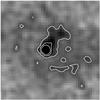 |
Fig. 8 Polar core at the center of IRAS 20077−0625. HST F606W image. The data have been binned to a resolution of |


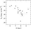 |
Fig. 9 Surface brightness vs. galactocentric radius. Filled and open symbols denote C-rich and O-rich envelopes, respectively. Circles are detections, triangles upper limits on the surface brightness. |
4. Discussion
4.1. Envelope surface brightness
4.1.1. Detectability of the envelopes
The detectability of an envelope in scattered ambient light depends on the effective optical depth for scattering, the strength of the radiation field, and the interstellar extinction along the line of sight. MH06 describe how the envelope opacity is conveniently parameterized by an estimate of the angular size of the optically thick plateau region using: 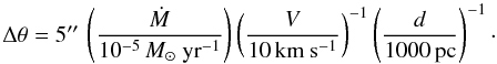 If this exceeds the resolution of the observations, the center of the envelope should attain maximum surface brightness.
Based on the parameters listed in Table 1, all the envelopes observed have  , as given by the above equation. They should therefore all be partly or fully resolved. If we consider the envelopes with good measurements (ignoring 4 with nominal upper limits due to the presence of a bright central star), there are 15 detections and three upper limits. One of the limits is sensitive, but it belongs to the envelope with the lowest Δθ, so it it probably just too small to be seen. The two other non-detections are for the two objects with the highest interstellar extinction (1.6 and 2.0 mag in B) which prevents reaching low intensity levels. Hence, if allowance is made for extinction, the characterization in terms of Δθ is a successful guide to detectability.
4.1.2. Envelope surface brightness and the interstellar radiation field
After correction for extinction, the peak surface brightness B0 shows a range of more than 2 mag (see Table 4). The scatter does not correlate with latitude (b) or height above the Galactic plane (z), and is not clearly related to Δθ or Ṁ. However, it does appear to depend partly on envelope chemistry and longitude (l), and both are found to result from a remarkable correlation with Galactic radius R.
Figure 9 shows the correlation of B0 with Galactic radius, with R calculated using the stellar distances and coordinates given in Table 1, and assuming R = 8.0 kpc for the Sun. It can be seen that the surface brightness decreases rapidly with R with an approximately linear relation. Omitting the upper limits for reasons mentioned above, a least squares fit gives:

and a residual rms scatter in B0 of 0.41, in units of mag arcsec-2. We interpret this relation to be the effect of a radial gradient in the interstellar radiation field. The linear dependence in magnitudes translates to an exponential law in the mean interstellar intensity. As far as we know, this is the most direct measurement so far of the gradient in the solar neighborhood. Our data suggest that the radiation field decreases by a factor of ~5 between R = 6 and R = 8 kpc. This is fairly consistent with the model of Mathis et al. (1983) who find a decrease of a factor of 7 between R = 5 kpc and the solar radius. A smaller factor of 3 is favored by the more recent study of Sodroski et al. (1997).
Inspection of Fig. 9 shows that the C-rich envelopes (filled symbols) follow essentially the same relation as the O-rich envelopes (open symbols). It would appear that the scattering properties of these different envelopes in the B-band are rather similar, and this is consistent with the similarities in the B − V colors measured in Sect. 3.3. We therefore interpret the observed difference in the average brightness of O-rich and C-rich envelopes in terms of their locations in the Galaxy. In our sample of AGB stars, the C-rich envelopes lie on average at larger values of R, and this is consistent with the higher relative fraction of carbon stars in the outer Galaxy (e.g., Jura et al. 1989). At larger Galactic radii, the C-rich envelopes are illuminated by a less intense radiation field.
4.2. Envelope morphology
4.2.1. Distribution of observed shapes
All the envelopes in Figs. 1–4 show relatively smooth radial profiles except for IRC+10216, which has sub-structure in the form of multiple arcs. However, IRC+10216 is much nearer than the other objects (see Table 1), so these could have similar structure which is not resolved at the larger distances. None of the envelopes show evidence for major, single-shell ejections which are seen in a few AGB envelopes and are thought to be caused by helium shell flashes (e.g., Olofsson et al. 2000).
As described in Sect. 3, the large scale shapes of the envelopes are roughly circular or elliptical, consistent with spherically or axially symmetric three dimensional structures seen in projection. The observed shapes are conveniently characterized by the ellipticities (E) listed in Table 4; recall, E = a/b (≥ 1.0), where a and b are the semi-major and semi-minor axes, respectively. The distribution of ellipticities for the sample (in order of increasing E) is shown in Fig. 10, which also indicates the formal 1-σ and 3-σ uncertainties. As explained in Sect. 3.4, the ellipticities we use to characterize the distribution refer to the overall shapes of the extended envelopes. If we use the shapes measured closer to the star (e.g., at 60% of the peak intensity), the distribution is similar to that in Fig. 10, but with somewhat higher ellipticities at the top end due mainly to the contribution of the core features in a few cases.
From Fig. 10, it can be seen that deviations of the overall shapes of the envelopes from circular symmetry are relatively small. Approximately half of the sample (47%) have E ≲ 1.1; 20% have E ≳ 1.2, and the rest are in between. The observed shapes of axially symmetric envelopes depend of course on the inclination angles, and they will appear circular when viewed end-on. However, there is no known bias in the inclinations of the observed envelopes, so we can assume them to be randomly oriented, with a median inclination of 60° to the line of sight, and rarely seen end-on. On this basis we can draw the following general conclusions on the 3-dimensional shapes of AGB envelopes: 1. A significant fraction (~half) are close to spherically symmetric. 2. At least 20% are significantly flattened. 3. Highly flattened, disk-like envelopes are relatively rare or non-existent. The results of Neri et al. (1998) based on observations of AGB envelopes in the millimeter lines of CO are in qualitative accord with our conclusions.
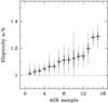 |
Fig. 10 Distribution of the measured large scale ellipticities of the AGB envelopes. The vertical error bars denote the formal 1-σ and 3-σ uncertainties. |
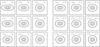 |
Fig. 11 Contour maps of model images for binary shaping. Left hand panel: variation of shape with Mc and i, for d = 10 AU and V = 10 km s-1. Right hand panel: variation of shape with Mc and d for i = 60° and V = 10 km s-1. |
4.2.2. Shaping mechanisms
There are two separate categories of shaping that can affect the morphology of the circumstellar envelopes: intrinsic shaping by or close to the central star, and interaction with the ISM. The latter can produce significant effects on large angular scales, typified by a one-sided bow shock due to the relative motion of the star and the surrounding medium.
We first consider whether the ISM interaction is likely to be important for the observed shapes by comparing estimates of the bow shock stand-off distance R0 for each object, taking into account the height above the Galactic plane, using Eqs. (2) and (5) of Cox et al. (2012), the stellar data in Table 1, and assuming a typical velocity relative to the ISM of 30 km s-1 (Feast & Whitelock 2000). We find that R0 for the envelopes observed ranges from ~1018 to 1020 cm, and exceeds the size scale corresponding to the angular radii (a) given in Table 4 by a median factor of 70, with a range of 30 to 3000. We conclude that interaction with ISM is unlikely to have a significant influence on the measured shapes. The observed morphologies are also consistent with this conclusion.
Our understanding of the intrinsic shaping mechanism of AGB envelopes is not well developed, but the expectation is that envelope shapes are different for single stars and binaries. Companions to AGB stars are, however, extremely difficult to detect (Jorissen & Frankowski 2008) and it is probable that hidden binaries are included in our sample.
For single AGB stars, which rotate very slowly, the zeroth order expectation is for spherically symmetric envelopes, although the extent of deviations caused by magnetic fields or related phenomena is not known. For AGB stars in binaries, the companion is expected to influence the shape in several ways. Close-in companions can cause tidal effects and spin-up, and modify the effective gravity of the star (e.g., Frankowski & Tylenda 2001). However, two additional effects are likely to be more important overall because they operate over a much wider range of separations: the flattening of the envelope by the gravitational field of the companion, and the effects of jets powered by accretion onto the companion.
Gravitational flattening.
The gravitational flattening of an envelope toward the orbital plane of a companion is a prominent feature of gas dynamical simulations of binary AGB systems (Mastrodemos & Morris 1999; Gawryszczak et al. 2002). Low mass companions or wide separations lead to nearly spherical envelopes, and close-in, high mass companions lead to flattened envelopes.
As a rough guide to the relation between envelope shape and binary parameters, Huggins et al. (2009) have obtained an approximate formula for the flattening in terms the companion mass Mc, the wind speed V, and the binary separation d, based on the simulations of Mastrodemos & Morris (1999). They use a highly simplified, axially symmetric model envelope with a density ~r-2, and characterized by a shape parameter K, where K = ne(r)/np(r) is the ratio of equatorial to polar density; the relation between K and the binary parameters is given in their Eq. (4). For an envelope illuminated by external radiation, they also give a prescription for the observed shape for a specified inclination of the symmetry axis to the line of sight (i). The observed shapes are given in terms of the ratio of column densities on the major and minor axes, Nmaj(θ)/Nmin(θ), but this can be shown to be equivalent the ellipticity (E) used in this paper.
To illustrate the range of binaries that could give rise to the observed shapes, Fig. 11 shows contour maps of synthetic images based on the simplified envelope model. The left hand panel shows the dependence of the observed shape on Mc and i for d = 10 AU. The right hand panel shows the dependence on Mc and d, for the median inclination (i = 60°). A representative value of V = 10 km s-1 is used for all cases.
It can be seen from the figures that the model produces envelope shapes that are qualitatively similar to those observed, i.e., with round or approximately elliptical contours. (The pinching effect on the minor axis of the flattest model is an artifact of the specific latitude dependence of density in the simple model, and is not expected to be a feature of real envelopes.) For masses ≲0.1 M⊙, the companion has essentially no effect at any angle, and the envelopes are very close to circular. For typical inclinations (i ~ 60°), companions with masses from 0.2 to 1.0 M⊙, significantly affect the envelopes, producing E ≳ 1.2 for separations up to 10 and 40 AU, respectively. Thus the range of observed envelope shapes is consistent with a spectrum of AGB stars ranging from single stars to binaries with relatively close companions of moderate mass.
Polar cores and jets.
The idea that binary companions are responsible for shaping the non-spherical envelopes is strengthened by the presence of the polar core asymmetries noted in Sect. 3. The fact that these elongated regions of enhanced radiation are seen in the central regions of approximately half of the sample (Table 4) is striking.
The best studied case is IRC+10216 (IRAS 09452+1330) where the effect is caused by the leakage of stellar radiation along bipolar axes close to the star, with one side much brighter than the other because of extinction (Skinner et al. 1998; Mauron & Huggins 2000). Other cases are probably similar (Sahai 2007), although in the absence of spectroscopy, localized emission cannot be ruled out.
The polar cores are not expected to be features of the mass loss of single stars, but they are expected in binary systems. One production mechanism is the diminution of mass loss along the polar directions which is an integral part of the binary shaping process, as seen in the simulations of Mastrodemos & Morris (1999). A second, related mechanism is the sculpting effect of jets from an accretion disk around the companion (e.g., Soker & Rappaport 2000). The effects of jets are seen in the Mira system (Josselin et al. 2000), and in a more extreme form in proto-PNe (e.g., Huggins et al. 2004). These mechanisms can act in parallel, and the dominant effect could vary from object to object.
Since polar cores and gravitational shaping likely arise from similar circumstances (i.e., the presence of a companion) there is good reason to suppose that they could be correlated. Our observations provide evidence for this view. The three envelopes with the highest ellipticities all have polar cores (Table 4). The polar cores are present in about half the sample, somewhat more than the fraction that are clearly flattened. It could be that the polar cores are formed by low as well as moderate mass companions, and are therefore more widely detectable. The relation between these features clearly warrants further study.
The high frequency of occurrence of polar cores in the observed sample also places interesting constraints on their physical origin. If they are intrinsic to envelope shaping, they will be permanent features of the envelopes. However, if they are caused by jets, the time evolution needs to be considered. Several cases where jets are suspected are discussed by Sahai (2007), and IRAS 01037+1219 (IRC+10011) has been modeled by Vinkovic et al. (2004) in terms of jets which have very recently turned on (≤ 200 yr) and are in the process of sculpting the envelope. Most of the cores observed here are small in radial extent, and with the high speed of jets, have comparably short time scales. Since we observe polar cores to be common, it is statistically unlikely that they have all formed within the last few hundred years. For the jet interpretation, the jets are likley to be weak or intermittent, so that the effects are local to the star. In this picture the more powerful jets seen in proto-PNe would develop later, when the companion interacts more strongly with the AGB star and accretes at a higher rate (Huggins 2007).
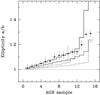 |
Fig. 12 Comparison of the observed ellipticities of the AGB sample with calculated distribution functions. The points are the observations, and the vertical error bars denote the 1-σ uncertainties. The upper and lower gray histograms are population synthesis predictions including the measurement errors for case 1 (g(q0) = 1) and case 2 ( |

4.2.3. Population synthesis
The question of binary shaping can be investigated further by comparing our observations of envelope shapes with the results of a recent population synthesis of AGB stars by Politano & Taam (2011). For a population consisting of single stars and binaries, they have calculated the distribution of the gravitational flattening parameter K of Huggins et al. (2009) described above. We have used their results to predict the distribution of the observed shapes of envelopes, assuming random orientations. Any contribution to the shaping by jets would be additional. We report the results in Fig. 12, using the median values of E in 15 quantiles, to represent the sample of observations.
The population synthesis assumes 50% of stars form as single stars and 50% from in binaries on the main sequence. For the binaries, we consider two representative cases for the assumed distribution of q0, the ratio of the secondary to primary mass on the main sequence. Case 1 is the standard case of Politano & Taam (2011) with a flat mass distribution, g(q0) = 1. Case 2 is a distribution that favors low mass companions with  . For case 1, 32% of the envelopes on the AGB are perturbed by a companion, and 68% are unperturbed (either single stars, or with distant companions); for case 2 these numbers are 18% and 82%, respectively.
If single stars produce exactly spherical envelopes, both cases 1 and 2 would have more than half the AGB envelopes with nominal ellipticities of E = 1.0 (in the absence of measurement errors). For realistic comparisons with the observations we include two effects. The gray histograms in Fig. 12 show the predicted distributions, where we include by simulation the effect of the average uncertainty in fitting the ellipses σ = ± 0.03. The black histograms in Fig. 12 show the two cases if we assume a residual ellipticity, normally distributed with mean 1.06 and dispersion ± 0.06 (1-σ) for all envelopes, in quadrature with any binary perturbation. This residual effect is chosen for illustration, and could arise from a combination of systematic effects such as residual asymmetric illumination and plate gradients, and as a natural dispersion in the true shapes of unperturbed envelopes.
In spite of the extreme simplicity of the underlying envelope model and the complexity of the population synthesis, it can be seen in Fig. 12 that the synthesized curves exhibit the qualitative characteristics of the observed distributions. The simulations suggest that the envelopes with ellipticities close to 1.0 are mainly unperturbed envelopes with a small dispersion in their shapes; and the less frequent, larger ellipticities are the results of binary interactions. There are significant quantitative differences in the predicted curves for the different assumptions about the binary mass ratios. It is encouraging that the observational data fall between the two cases shown, but the observational sample is too small to discriminate between them at this stage.
From an empirical point of view, if the polar cores indicate binaries as we suggest, the observation of cores in half the sample would indicate a somewhat greater percentage of AGB binaries than predicted by the population synthesis. A larger sample would be important to investigate this further.
4.3. AGB stars as precursors of PNe
The evidence for a hidden population of AGB binaries provided by our observations is of interest for understanding post-AGB evolution. In particular, the importance of binaries in shaping planetary nebulae (PNe) is a subject that is widely debated (De Marco 2009), and it is uncertain whether a binary companion is an essential ingredient for PN formation. It is observed that 12–21% of PNe have close binary companions (Miszalski et al. 2009) and these have evidently passed through a common envelope phase. Other companions at larger distances may be present, but have so far proved elusive to observation (e.g., Hrivnak et al. 2011).
The objects in our sample of AGB stars with high mass loss rates are expected to be the immediate precursors of PNe. We find that ~20% of the envelopes already show significant shaping effects that we attribute to the presence of substantial companions. We also find evidence for additional, more subtle shaping effects in the form of polar cores in up 50% of envelopes, which also probably arise from companions (including low mass companions). These numbers are preliminary because the sample size is small, but they demonstrate that detailed observations of AGB envelopes have the potential to characterize aspects of the interactions that contribute to the shaping of PNe.
5. Conclusions
We have carried out a deep imaging survey of 22 AGB stars with high mass loss rates in order to investigate the geometry of their circumstellar envelopes. We report the detection of 15 envelopes in dust-scattered Galactic radiation, and we characterize their properties in terms of the surface brightness, radial intensity profile, and observed shape.
We find that the surface brightness of the envelopes shows a rapid decrease with Galactic radius, which we interpret as a steep gradient in the interstellar radiation field. As far as we know, this is the most direct observation of this gradient in the solar neighborhood.
The envelopes show a range of geometries: approximately half are close to spherically symmetric, and ~20% are distinctly elliptical. We interpret the shapes in terms of populations of single stars and binaries whose envelopes are flattened by a companion. The observed distribution of the ellipticities of the envelopes is qualitatively consistent with the results of population synthesis models. We also find that approximately half the sample of envelopes exhibit small-scale, polar cores which we interpret as the escape of starlight through polar holes produced by companions.
Our observations of envelope flattening and polar holes point to a hidden population of binary companions within the circumstellar envelopes of AGB stars. These companions affect the geometry of the envelopes on the AGB, and are potentially important guides to the evolutionary channels that lead to binaries observed in the post-AGB phase.
Online material
Appendix A: Envelope non-detections
Images of the fields for which the AGB star but not the envelope are detected are shown in Fig. A.1. IRAS 06012+0726 (AFGL 865) is not detected in V or I, and is not shown. It is however well detected in J, H, and K in the 2MASS survey, with J = 13.38, H = 9.28, and K = 6.06. At a Galactic latitude b = −7, this object has the largest extinction (AV ~ 1.6 mag) based on the NED extinction calculator, which probably accounts for the non-detection at short wavelengths.
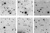 |
Fig. A.1 Images of objects with non-detection of the envelope. Ticks indicate the AGB star. Top row, left to right: IRAS 00193−4033 (AFGL 5017), EFOSC2 V-band image. IRAS 04575+1251 (AFGL 5134), EFOSC2 V-band image. IRAS 05418−3224, EFOSC2 B-band image. Bottom row, left to right: IRAS 06255−4928, EFOSC2 B-band image. IRAS 09521−7508, EMMI B-band image. IRAS 20042−4241, EMMI B-band image. |
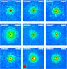 |
Fig. 5 Images of the circumstellar envelopes. The images are shown in color with the field stars replaced, and with the contours of Figs. 1–4 superposed. Top row, left to right: IRAS 01037+1219, V-band; IRAS 07454−7112, B-band; IRAS 09116−2439, B-band. Middle row, left to right: IRAS 09452+1330, V-band; IRAS 10323−4611, B-band; IRAS 12384−4536, V-band. Bottom row, left to right: IRAS 14591−4438, B-band; IRAS 16029−3041, V-band; IRAS 17319−6234, V-band. All images are square, with north to the top and east to the left. |
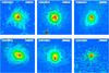 |
Fig. 6 Continuation of Fig. 5. Top row, left to right: IRAS 18240+2326, V-band; IRAS 18467−4802, F606W; IRAS 19178−2620, B-band. Bottom row, left to right: IRAS 20077−0625, V-band; IRAS 23257+1038, V-band; IRAS 23320+4316, B-band. All images are square, with north to the top and east to the left. |
Acknowledgments
We acknowledge the use of the MIDAS software from ESO which was used for the data processing. The HST data were obtained from the ESA/ESO ST-ECF Archive Center at Garching, Germany. This work was supported in part by NSF grant AST 08-06910 (to P.J.H.).
References
- Castro-Carrizo, A., Quintana-Lacaci, G., Neri, R., et al. 2010, A&A, 523, A59 [NASA ADS] [CrossRef] [EDP Sciences] [Google Scholar]
- Cox, N. L. J., Kerschbaum, F., van Marle, A.-J., et al. 2012, A&A, 537, A35 [NASA ADS] [CrossRef] [EDP Sciences] [Google Scholar]
- David, P., Le Squeren, A. M., & Sivagnanam, P. 1993, A&A, 277, 453 [NASA ADS] [Google Scholar]
- De Marco, O. 2009, PASP, 121, 316 [NASA ADS] [CrossRef] [Google Scholar]
- Decin, L., Royer, P., Cox, N. L. J., et al. 2011, A&A, 534, A1 [NASA ADS] [CrossRef] [EDP Sciences] [Google Scholar]
- Feast, M. W., & Whitelock, P. A. 2000, MNRAS, 317, 460 [NASA ADS] [CrossRef] [Google Scholar]
- Frankowski, A., & Tylenda, R. 2001, A&A, 367, 513 [NASA ADS] [CrossRef] [EDP Sciences] [Google Scholar]
- Gawryszczak, A. J., Mikolajewska, K., & Rózyczka, M. 2002, A&A, 385, 205 [NASA ADS] [CrossRef] [EDP Sciences] [Google Scholar]
- Groenewegen, M. A. T., Sevenster, M., Spoon, H. W. W., & Pérez, I. 2002, A&A, 390, 511 [NASA ADS] [CrossRef] [EDP Sciences] [Google Scholar]
- Habing, H. J., & Olofsson, H. 2004, AGB Stars, A&A Library (Berlin: Springer) [Google Scholar]
- Hrivnak, B. J., Lu, W., Bohlender, D., et al. 2011, ApJ, 734, 25 [NASA ADS] [CrossRef] [Google Scholar]
- Huggins, P. J. 2007, ApJ, 663, 342 [NASA ADS] [CrossRef] [Google Scholar]
- Huggins, P. J., Muthu, C., Bachiller, R., Forveille, T., & Cox, P. 2004, A&A, 414, 581 [NASA ADS] [CrossRef] [EDP Sciences] [Google Scholar]
- Huggins, P. J., Mauron, N., & Wirth, E. A. 2009, MNRAS, 396, 1805 [NASA ADS] [CrossRef] [Google Scholar]
- Jackson, T., Ivezić, Ž., & Knapp, G. R. 2002, MNRAS, 337, 749 [NASA ADS] [CrossRef] [Google Scholar]
- Jorissen, A. 2004, AGB Stars, eds. H. J. Habing, & H. Olofsson, A&A Library (Berlin: Springer), 461 [Google Scholar]
- Jorissen, A., & Frankowski, A. 2008, AIP Conf. Ser., 1057, 1 [NASA ADS] [CrossRef] [Google Scholar]
- Josselin, E., Mauron, N., Planesas, P., & Bachiller, R. 2000, A&A, 362, 255 [NASA ADS] [Google Scholar]
- Jura, M., Joyce, R. R., & Kleinmann, S. G. 1989, ApJ, 336, 924 [Google Scholar]
- Kerschbaum, F., Lebzelter, T., & Wing, R. F. 2011, Why Galaxies Care about AGB Stars II: Shining Examples and Common Inhabitants, ASP Conf. Ser., 445 [Google Scholar]
- Lagadec, E., Verhoelst, T., Mékarnia, D., et al. 2011, MNRAS, 417, 32 [NASA ADS] [CrossRef] [Google Scholar]
- Leao, I. C., de Laverny, P., Chesneau, O., et al. 2006, A&A, 455, 187 [NASA ADS] [CrossRef] [EDP Sciences] [Google Scholar]
- Loup, C., Forveille, T., Omont, A., & Paul, J. P. 1993, A&AS, 99, 291 [NASA ADS] [Google Scholar]
- Marengo, M. 2009, PASA, 26, 365 [NASA ADS] [CrossRef] [Google Scholar]
- Martin, P. G., & Rogers, C. 1987, ApJ, 322, 374 [NASA ADS] [CrossRef] [Google Scholar]
- Mastrodemos, N., & Morris, M. 1999, ApJ, 523, 357 [NASA ADS] [CrossRef] [Google Scholar]
- Mathis, J. S., Mezger, P. G., & Panagia, N. 1983, A&A, 128, 212 [NASA ADS] [Google Scholar]
- Mauron, N., & Huggins, P. J. 1999, A&A, 349, 203 [NASA ADS] [Google Scholar]
- Mauron, N., & Huggins, P. J. 2000, A&A, 359, 707 [NASA ADS] [Google Scholar]
- Mauron, N., & Huggins, P. J. 2006, A&A, 452, 257 [NASA ADS] [CrossRef] [EDP Sciences] [Google Scholar]
- Miszalski, B., Acker, A., Moffat, A. F. J., Parker, Q. A., & Udalski, A. 2009, A&A, 496, 813 [NASA ADS] [CrossRef] [EDP Sciences] [Google Scholar]
- Monet, D. G., Levine, S. E., Canzian, B., et al. 2003, AJ, 125, 984 [NASA ADS] [CrossRef] [Google Scholar]
- Morris, M., Sahai, R., Matthews, K., et al. 2006, Planetary Nebulae in our Galaxy and Beyond, eds. M. Barlow, & R. Mendez, IAU Symp., 234, 469 [Google Scholar]
- Neri, R., Kahane, C., Lucas, R., et al. 1998, A&AS, 130, 1 [NASA ADS] [CrossRef] [EDP Sciences] [Google Scholar]
- Olivier, E. A., Whitelock, P., & Marang, F. 2001, MNRAS, 326, 490 [NASA ADS] [CrossRef] [Google Scholar]
- Olofsson, H., Bergman, P., Lucas, R., et al. 2000, A&A, 353, 583 [NASA ADS] [Google Scholar]
- Politano, M., & Taam, R. E. 2011, ApJ, 741, 5 [NASA ADS] [CrossRef] [Google Scholar]
- Ramstedt, S., Schöier, F. L., Olofsson, H., & Lundgren, A. A. 2008, A&A, 487, 645 [NASA ADS] [CrossRef] [EDP Sciences] [Google Scholar]
- Sahai, R. 2007, Asymmetrical Planetary Nebulae IV, eds. R. L. M. Corradi, A. Manchado, & N. Soker, I.A.C., 421 [Google Scholar]
- Schöier, F. L., & Olofsson, H. 2001, A&A, 368, 969 [NASA ADS] [CrossRef] [EDP Sciences] [Google Scholar]
- Sérsic, J. L. 1963, BAAA, 6, 41 [Google Scholar]
- Skinner, C. J., Meixner, M., & Bobrowsky, M. 1998, MNRAS, 300, L29 [NASA ADS] [CrossRef] [Google Scholar]
- Snodgrass, C. 2009, ESO NTT Documentation LSO-LIS-ESO-40500-0002 [Google Scholar]
- Sodroski, T. J., Odegard, N., Arendt, R. G., et al. 1997, ApJ, 480, 173 [NASA ADS] [CrossRef] [Google Scholar]
- Soker, N., & Rappaport, S. 2000, ApJ, 538, 241 [NASA ADS] [CrossRef] [Google Scholar]
- Theuns, T., & Jorissen, A. 1993, MNRAS, 265, 946 [NASA ADS] [CrossRef] [Google Scholar]
- Vinković, D., Blöcker, T., Hofmann, K.-H., Elitzur, M., & Weigelt, G. 2004, MNRAS, 352, 852 [NASA ADS] [CrossRef] [Google Scholar]
- Whitelock, P., Menzies, J., Feast, M., et al. 1994, MNRAS, 267, 711 [NASA ADS] [CrossRef] [Google Scholar]
All Tables
All Figures
|
Fig. 1 Images and radial profiles of the AGB envelopes. Each row shows from left to right: the image in grayscale; a close-up contour map of the envelope, with field stars removed and their cores masked; and the radial profile of the envelope with the PSF. The field size is indicated in the images. The filters and contours, specified by the lowest contour (and contour interval) in units of the peak surface brightness of the envelope, are as follows (from top to bottom): IRAS 01037+1219, V-band, contours 0.33 (0.43); IRAS 07454−7112, B-band, contours 0.31 (0.23); IRAS 09116−2439, B-band, contours 0.28 (0.26); IRAS 09452+1330, V-band, contours 0.32 (0.16). The images are square, with north to the top and east to the left. |
| In the text | |
|
Fig. 2 Continuation of Fig. 1. From top to bottom: IRAS 10323−4611, B-band, contours 0.13 (0.25); IRAS 12384−4536, V-band, contours 0.25 (0.25); IRAS 14591−4438, B-band, contours 0.35 (0.33); IRAS 16029−3041, V-band, contours 0.17 (0.17). The images are square, with north to the top and east to the left. |
| In the text | |
|
Fig. 3 Continuation of Fig. 1. From top to bottom: IRAS 17319−6234, V-band, contours 0.12 (0.19); IRAS 18240+2326, V-band, contours 0.34 (0.23); IRAS 18467−4802, F606W (HST/ACS), contours 0.27 (0.25); IRAS 19178−2620, B-band, contours 0.18 (0.22). The images are square, with north to the top and east to the left. |
| In the text | |
|
Fig. 4 Continuation of Fig. 1. From top to bottom: IRAS 20077−0625, V-band, contours 0.20 (0.18); IRAS 23257+1038, V-band, contours 0.20 (0.31); IRAS 23320+4316, B-band, contours 0.29 (0.29). The images are square, with north to the top and east to the left. |
| In the text | |
|
Fig. 7 Contour fitting for IRAS 17319−6234. The inner (gray) and outer (black) crosses sample the envelope at 10° intervals in azimuth and at 20% and 40% of the peak intensity, respectively. Gaps in the data correspond to masked regions of the image. The curves show the fitted ellipses; the small inner circles show the fitted centers. |
| In the text | |
|
Fig. 8 Polar core at the center of IRAS 20077−0625. HST F606W image. The data have been binned to a resolution of |
| In the text | |
|
Fig. 9 Surface brightness vs. galactocentric radius. Filled and open symbols denote C-rich and O-rich envelopes, respectively. Circles are detections, triangles upper limits on the surface brightness. |
| In the text | |
|
Fig. 10 Distribution of the measured large scale ellipticities of the AGB envelopes. The vertical error bars denote the formal 1-σ and 3-σ uncertainties. |
| In the text | |
|
Fig. 11 Contour maps of model images for binary shaping. Left hand panel: variation of shape with Mc and i, for d = 10 AU and V = 10 km s-1. Right hand panel: variation of shape with Mc and d for i = 60° and V = 10 km s-1. |
| In the text | |
|
Fig. 12 Comparison of the observed ellipticities of the AGB sample with calculated distribution functions. The points are the observations, and the vertical error bars denote the 1-σ uncertainties. The upper and lower gray histograms are population synthesis predictions including the measurement errors for case 1 (g(q0) = 1) and case 2 ( |
| In the text | |
|
Fig. A.1 Images of objects with non-detection of the envelope. Ticks indicate the AGB star. Top row, left to right: IRAS 00193−4033 (AFGL 5017), EFOSC2 V-band image. IRAS 04575+1251 (AFGL 5134), EFOSC2 V-band image. IRAS 05418−3224, EFOSC2 B-band image. Bottom row, left to right: IRAS 06255−4928, EFOSC2 B-band image. IRAS 09521−7508, EMMI B-band image. IRAS 20042−4241, EMMI B-band image. |
| In the text | |
|
Fig. 5 Images of the circumstellar envelopes. The images are shown in color with the field stars replaced, and with the contours of Figs. 1–4 superposed. Top row, left to right: IRAS 01037+1219, V-band; IRAS 07454−7112, B-band; IRAS 09116−2439, B-band. Middle row, left to right: IRAS 09452+1330, V-band; IRAS 10323−4611, B-band; IRAS 12384−4536, V-band. Bottom row, left to right: IRAS 14591−4438, B-band; IRAS 16029−3041, V-band; IRAS 17319−6234, V-band. All images are square, with north to the top and east to the left. |
| In the text | |
|
Fig. 6 Continuation of Fig. 5. Top row, left to right: IRAS 18240+2326, V-band; IRAS 18467−4802, F606W; IRAS 19178−2620, B-band. Bottom row, left to right: IRAS 20077−0625, V-band; IRAS 23257+1038, V-band; IRAS 23320+4316, B-band. All images are square, with north to the top and east to the left. |
| In the text | |
Current usage metrics show cumulative count of Article Views (full-text article views including HTML views, PDF and ePub downloads, according to the available data) and Abstracts Views on Vision4Press platform.
Data correspond to usage on the plateform after 2015. The current usage metrics is available 48-96 hours after online publication and is updated daily on week days.
Initial download of the metrics may take a while.