| Issue |
A&A
Volume 550, February 2013
|
|
|---|---|---|
| Article Number | L8 | |
| Number of page(s) | 4 | |
| Section | Letters | |
| DOI | https://doi.org/10.1051/0004-6361/201220847 | |
| Published online | 28 January 2013 | |
Lopsided dust rings in transition disks
1
Excellence Cluster Universe, Technische Universität München,
Boltzmannstr. 2,
85748
Garching,
Germany
2
Harvard-Smithsonian Center for Astrophysics, 60 Garden Street, Cambridge,
MA
02138,
USA
e-mail:
This email address is being protected from spambots. You need JavaScript enabled to view it.
3
Heidelberg University, Center for Astronomy (ZAH), Institute for
Theoretical Astrophysics, Albert
Ueberle Str. 2, 69120
Heidelberg,
Germany
Received:
4
December
2012
Accepted:
9
January
2013
Abstract
Context. Particle trapping in local or global pressure maxima in protoplanetary disks is one of the new paradigms in the theory of the first stages of planet formation. However, finding observational evidence for this effect is not easy. Recent work suggests that the large ring-shaped outer disks observed in transition disk sources may in fact be lopsided and constitute large banana-shaped vortices.
Aims. We wish to investigate how effectively dust can accumulate along the azimuthal direction. We also want to find out if the size-sorting resulting from this accumulation can produce detectable signatures at millimeter wavelengths.
Methods. To keep the numerical cost under control we developed a 1+1D method in which the azimuthal variations are treated separately from the radial variations. The azimuthal structure was calculated analytically for a steady-state between mixing and azimuthal drift. We derived equilibration time scales and compared the analytical solutions to time-dependent numerical simulations.
Results. We found that weak, but long-lived azimuthal density gradients in the gas can induce very strong azimuthal accumulations of dust. The strength of the accumulations depends on the Péclet number, which describes the relative importance of advection and diffusion. We applied our model to transition disks and our simulated observations show that this effect would be easily observable with the Atacama Large Millimeter/submillimeter Array (ALMA) and could be used to put constraints on the strength of turbulence and the local gas density.
Key words: accretion, accretion disks / protoplanetary disks / stars: pre-main sequence / planets and satellites: formation / submillimeter: planetary systems / circumstellar matter
© ESO, 2013
1. Introduction
The process of planet formation is thought to start with the growth of dust aggregates in a protoplanetary disk through coagulation (see, e.g., the review by Blum & Wurm 2008). The idea is that these aggregates get successively bigger until either gravoturbulent processes set in (Goldreich & Ward 1973; Johansen et al. 2007; Cuzzi et al. 2008) or planetesimals are formed directly via coagulation (Weidenschilling 1977; Okuzumi et al. 2012; Windmark et al. 2012). One of the main unsolved problems in these scenarios is excessive radial drift (Weidenschilling 1977; Nakagawa et al. 1986; Brauer et al. 2007). The origin of this problem lies in the sub-Keplerian motion of the gas in the disk, caused by the inward-pointing pressure gradient. The dust particles in the disk, however, feel only the friction with the sub-Keplerian gas and as they grow to larger sizes, the reduced surface-to-mass ratio causes them to fall toward the star with speeds of up to 50 m s-1 (Whipple 1972; Weidenschilling 1977). Thus, if a particle grows, it will sooner or later get “flushed” toward the star before it can grow very large (Brauer et al. 2008; Birnstiel et al. 2010, 2012). This is what we call the radial drift barrier, and this still poses one of the main unsolved problems of the early phases of planet formation.
A possible solution to this problem might lie in the concept of “particle traps”. This idea was proposed some time ago in the context of anticyclonic vortices by Barge & Sommeria (1995) and Klahr & Henning (1997), and in the context of turbulent eddies (Johansen & Klahr 2005; Cuzzi & Hogan 2003). These vortex- or eddy-related local pressure maxima act as particle traps because particles tend to drift towards higher pressure. In the case of vortices and eddies they act on small scales. Particle traps on a global disk scale have been proposed as well (Whipple 1972; Rice et al. 2006; Alexander & Armitage 2007; Garaud 2007; Kretke & Lin 2007; Dzyurkevich et al. 2010) and are shown to be conducive to planet formation (Brauer et al. 2008). Intermediate scale particle traps may also occur from magnetorotationally driven turbulence: the so-called zonal flows (Johansen et al. 2009).
If we want to test by observations whether this scenario of particle trapping actually occurs in nature, we are faced with a problem. The terrestrial planet-forming region around a pre-main sequence star is usually too small on the sky to be spatially sufficiently resolved to test this trapping scenario. Moreover, the optical depth of this inner disk region is likely to be too large to be able to probe the mid-plane region of the disk. Fortunately, what constitutes the “meter-size drift-barrier” at 1 AU is a “centimeter-size drift-barrier” at ~50 AU. Those disk regions are optically thin at millimeter (mm) wavelength and particles in the mm size range can be spectroscopically identified by studying the mm spectral slope (Testi et al. 2001; Natta et al. 2004; Ricci et al. 2010a,b). So the goal that has been pursued recently is to identify observational signatures of dust particle trapping of millimeter-sized particles in the outer regions of disks, as a proxy of what happens in the unobservable inner regions of the disk (Pinilla et al. 2012b,a). The Pinilla et al. (2012a) paper suggests that the huge mm continuum rings observed in most of the transition disks (Piétu et al. 2006; Brown et al. 2008; Hughes et al. 2009; Isella et al. 2010; Andrews et al. 2011), may in fact be large global particle traps caused by the pressure bump resulting from, for example, a massive planet opening up a gap.
In these papers we have focused on the intermediate-scale (zonal-flow-type) and the large-scale (global) pressure bumps, simply because current capabilities of mm observatories (including ALMA) are not yet able to resolve small-scale structures such as vortices. The vortex trapping scenario thus appears to remain observationally out of reach. However, a closer look at the mm maps of transition disks suggest that some of them may exhibit a deviation from axial symmetry. For instance, the observations presented in Mayama et al. (2012) or the mm images of Brown et al. (2009) suggests a lopsided banana-shaped ring instead of a circular ring. Regály et al. (2012) proposed that these banana-shaped rings are in fact a natural consequence of mass piled up at some obstacle in the disk. Once the resulting ring becomes massive enough, it becomes Rossby-unstable and a large banana-shaped vortex is formed that periodically fades and re-forms with a maximum azimuthal gas density contrast of a factor of a few. Regály et al. (2012) showed that this naturally leads to lopsided rings seen in mm wavelength maps (see also earlier work by Wolf & Klahr 2002) on radiative transfer predictions of observability of vortices with ALMA). The formation of such Rossby-wave induced vortices was previously demonstrated by Lyra et al. (2009), who showed that they may in fact (when they are situated much farther inward, in the planet forming region) lead to the rapid formation of planetary embryos of Marsmass. Sándor et al. (2011) subsequently showed that this scenario may rapidly produce a 10 Earth-mass planetary core.
The goal of the current letter is to combine the scenario of forming a lopsided gas ring (e.g., Regály et al. 2012) with the scenario of particle trapping and growth presented by Pinilla et al. (2012a). In Sect. 2 we will outline the physical effects involved and derive analytical solutions to the dust distribution along the non-axisymmetric pressure bump and in Sect. 3 we will test the observability of these structures in resolved (sub-)mm imaging and in the mm spectral index. Our findings will be summarized in Sect. 4.
2. Analytical model
Dust particles embedded in a gaseous disk feel drag forces if they move relatively to the gas. The radial and azimuthal equations of motion have been solved, for example, by Weidenschilling (1977) or Nakagawa et al. (1986) for the case of an axisymmetric, laminar disk. It was found that particles drift inward towards higher pressure. In this paper we will focus on the case where a non-axisymmetric structure has formed a long-lived, non-axisymmetric pressure maximum in the disk. This pressure maximum is able to trap inward-spiralling dust particles. As was done in the aforementioned works, we can solve for a stationary drift velocity, but contrary to the calculations of Nakagawa et al. (1986), the radial pressure gradient is zero at the pressure maximum while the azimuthal pressure gradient can be different from zero. This leads again to a systematic drift motion of the dust particles towards the pressure maximum, but now in azimuthal instead of in radial direction.
The equations of motion in polar coordinates relative to the Keplerian motion become (see
Nakagawa et al. 1986)

 where
ud,r and
ud,φ are the r and
φ components of the dust velocity, respectively,
ug,r and
ug,φ the r and
φ components of the gas, Ωk the Keperian frequency,
P the gas pressure, and ρd and
ρg the dust and gas densities; A denotes the
drag coefficient (see Nakagawa et al. 1986, Eqs.
(2.3) and (2.4)). Solving the above equations for the velocity along the φ
direction at the mid-plane (z = 0) gives
where
ud,r and
ud,φ are the r and
φ components of the dust velocity, respectively,
ug,r and
ug,φ the r and
φ components of the gas, Ωk the Keperian frequency,
P the gas pressure, and ρd and
ρg the dust and gas densities; A denotes the
drag coefficient (see Nakagawa et al. 1986, Eqs.
(2.3) and (2.4)). Solving the above equations for the velocity along the φ
direction at the mid-plane (z = 0) gives  (5)where
X = ρd/ρg
is the dust-to-gas ratio, Vk the Keplerian velocity, and the
Stokes number1 is given by
(5)where
X = ρd/ρg
is the dust-to-gas ratio, Vk the Keplerian velocity, and the
Stokes number1 is given by 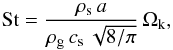 (6)with
ρs as internal density of the dust, particle radius
a, and the isothermal sound speed cs. Dust is
advected with the velocity given in Eq. (5),
but it is also turbulently stirred. Together, the evolution of the dust density along the
ring is then described by
(6)with
ρs as internal density of the dust, particle radius
a, and the isothermal sound speed cs. Dust is
advected with the velocity given in Eq. (5),
but it is also turbulently stirred. Together, the evolution of the dust density along the
ring is then described by 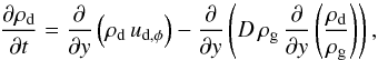 (7)where
y = r φ is the coordinate along the
ring circumference. We use a dust diffusion coefficient D according to
Youdin & Lithwick (2007),
D = Dgas/(1 + St2),
where we assume the gas diffusivity to be equal to the gas viscosity, taken to be
(7)where
y = r φ is the coordinate along the
ring circumference. We use a dust diffusion coefficient D according to
Youdin & Lithwick (2007),
D = Dgas/(1 + St2),
where we assume the gas diffusivity to be equal to the gas viscosity, taken to be
 , with
αt as the turbulence parameter (see Shakura & Sunyaev 1973). Equation (7) can be integrated forward in time numerically, but assuming that the
turbulent mixing and the drift term have reached an equilibrium, and also assuming a low
dust-to-gas ratio, we can analytically solve for the dust density in a steady-state between
mixing and drifting, which yields
, with
αt as the turbulence parameter (see Shakura & Sunyaev 1973). Equation (7) can be integrated forward in time numerically, but assuming that the
turbulent mixing and the drift term have reached an equilibrium, and also assuming a low
dust-to-gas ratio, we can analytically solve for the dust density in a steady-state between
mixing and drifting, which yields ![Mathematical equation: \begin{equation} \rhodust(y) = C \, \rhogas(y) \, \exp\left[ -\frac{\St(y)}{\alphat}\right], \label{eq:rhodust_analytical} \end{equation}](/articles/aa/full_html/2013/02/aa20847-12/aa20847-12-eq20.png) (8)where C is
a normalization constant and St(y) is the Stokes number which depends on
y via the changes in gas density. Equation (8) thus predicts the distribution of dust for any given profile of the
gas density ρg. The contrast between the position of the
azimuthal pressure maximum and its surrounding then gives
(8)where C is
a normalization constant and St(y) is the Stokes number which depends on
y via the changes in gas density. Equation (8) thus predicts the distribution of dust for any given profile of the
gas density ρg. The contrast between the position of the
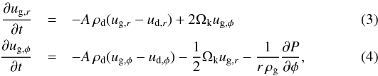
azimuthal pressure maximum and its surrounding then gives ![Mathematical equation: \begin{equation} \frac{\rhodust^\mathrm{max}}{\rhodust^\mathrm{min}} =\frac{\rhogas ^\mathrm{max}}{\rhogas ^\mathrm{min}} \, \exp\left[\frac{\St^\mathrm{min}-\St^\mathrm{max}}{\alphat}\right], \label{eq:enhancement} \end{equation}](/articles/aa/full_html/2013/02/aa20847-12/aa20847-12-eq24.png) (9)which is plotted in Fig.
1. The Stokes numbers at the pressure maximum and
minimum are Stmax and Stmin (note:
Stmax < Stmin). It can be seen that once the
particle’s Stokes number becomes larger than the turbulence parameter
αt, the dust concentration becomes much stronger than the gas
concentration.
(9)which is plotted in Fig.
1. The Stokes numbers at the pressure maximum and
minimum are Stmax and Stmin (note:
Stmax < Stmin). It can be seen that once the
particle’s Stokes number becomes larger than the turbulence parameter
αt, the dust concentration becomes much stronger than the gas
concentration.
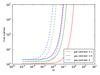 |
Fig. 1 Contrast between the dust density in the azimuthal maximum and its surroundings for
different gas density contrasts ( |

However, the time scales on which these concentrations are reached can be significant. To
get an estimate for this time scale, we compare the advection time scale
tadv = L/u
and the diffusion time scale
tdiff = L2/D
with velocity u and length scale L. The ratio of these
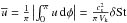
time scales is known as the Péclet number Pe and using Eq. (5), can be written as 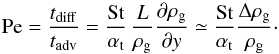 (10)It describes the
relative importance of advection and diffusion and confirms that dust accumulations occur
only for particles with St ≳ αt, because otherwise diffusion
dominates over advection which means that variations in the dust-to-gas ratio are being
smeared out. It also shows that for those large particles the advection time scale is the
shorter one, thus setting the time scale of the concentration process, which can be written
as
(10)It describes the
relative importance of advection and diffusion and confirms that dust accumulations occur
only for particles with St ≳ αt, because otherwise diffusion
dominates over advection which means that variations in the dust-to-gas ratio are being
smeared out. It also shows that for those large particles the advection time scale is the
shorter one, thus setting the time scale of the concentration process, which can be written
as  (11)where
H = cs/Ωk is
the pressure scale height, and we have used a mean velocity
(11)where
H = cs/Ωk is
the pressure scale height, and we have used a mean velocity
 , with
 (12)which for
St < 1 simplifies to
δSt = Stmin − Stmax. Furthermore, we define the
pressure maximum and minimum to be at φ = 0 and
φ = π, respectively. As an example, at 35 AU, for
H/r = 0.07, a Stokes number of 0.2,
and a gas density contrast of
(12)which for
St < 1 simplifies to
δSt = Stmin − Stmax. Furthermore, we define the
pressure maximum and minimum to be at φ = 0 and
φ = π, respectively. As an example, at 35 AU, for
H/r = 0.07, a Stokes number of 0.2,
and a gas density contrast of  , the time
scale is 3 × 10⁵ years, but could be as short as 102 orbits for
optimal conditions. Any gas structure therefore has to be long-lived to cause strong
asymmetries in the dust, making the asymmetries caused by a planet or long-lived vortices
the best candidates (Meheut et al. 2012). If such an
accumulation is formed and the gas asymmetry disappears, it still takes
tdiff to “remove” it, which at 35 AU is of the order of Myrs.
It remains to be shown whether short-lived, but reoccurring structures like zonal flows are
able to induce strong dust accumulations.
, the time
scale is 3 × 10⁵ years, but could be as short as 102 orbits for
optimal conditions. Any gas structure therefore has to be long-lived to cause strong
asymmetries in the dust, making the asymmetries caused by a planet or long-lived vortices
the best candidates (Meheut et al. 2012). If such an
accumulation is formed and the gas asymmetry disappears, it still takes
tdiff to “remove” it, which at 35 AU is of the order of Myrs.
It remains to be shown whether short-lived, but reoccurring structures like zonal flows are
able to induce strong dust accumulations.
 |
Fig. 2 Azimuthal steady-state solutions for small dust grains (red line) and large dust grains (blue line) for a given sinusoidal gas profile (black line, identical with red line). Dashed lines show numerical solutions at 1, 2, and 5 advection time scales. |
3. Simulated observations
In the following, we will evaluate whether the dust structures we expect would be
observable in resolved mm images of ALMA. We used the results of Pinilla et al. (2012a) for the radial profile of the gas surface density
 and temperature
T(r). These simulations represent a disk of mass
Mdisk = 0.05 M⊙ around a solar
mass star with a 15 Jupiter-mass planet at 20 AU. For simplicity, as two-dimensional gas
surface density we used
and temperature
T(r). These simulations represent a disk of mass
Mdisk = 0.05 M⊙ around a solar
mass star with a 15 Jupiter-mass planet at 20 AU. For simplicity, as two-dimensional gas
surface density we used ![Mathematical equation: \begin{eqnarray} \label{eq:gas_profile} &&\Siggas(r,\phi) = \overline{\Sigma}_\mathrm{g}(r) \, \left[1 + A(r) \, \sin\left(\phi - \frac{\pi}{2}\right)\right]\\ &&A(r) = \frac{c-1}{c+1}\, \exp\left[-\frac{\left(r-R_\mathrm{s}\right)^2}{2\,H^2}\right], \end{eqnarray}](/articles/aa/full_html/2013/02/aa20847-12/aa20847-12-eq54.png) where
c = Σg,max/Σg,min
is the largest contrast of the gas surface density, taken to be 1.5 and
Rs is the position of the radial pressure bump. The dust size
distribution Σd(r,a) was also taken from the simulations of
Pinilla et al. (2012a) and distributed azimuthally
using the analytical solution from Eq. (8)
(see Fig. 2). We also confirmed the analytical solution
and time scales by solving Eq. (7)
numerically, as shown in Fig. 2. Strictly speaking,
this analytical solution only holds at the position of the radial pressure bump, but since
most of the mm emission comes from the large grains which in the simulations of Pinilla et al. (2012a) are trapped near the radial
pressure maximum, this should be a reasonable approximation. Full 2D simulations will be
needed to confirm this and to investigate the effects of shear.
where
c = Σg,max/Σg,min
is the largest contrast of the gas surface density, taken to be 1.5 and
Rs is the position of the radial pressure bump. The dust size
distribution Σd(r,a) was also taken from the simulations of
Pinilla et al. (2012a) and distributed azimuthally
using the analytical solution from Eq. (8)
(see Fig. 2). We also confirmed the analytical solution
and time scales by solving Eq. (7)
numerically, as shown in Fig. 2. Strictly speaking,
this analytical solution only holds at the position of the radial pressure bump, but since
most of the mm emission comes from the large grains which in the simulations of Pinilla et al. (2012a) are trapped near the radial
pressure maximum, this should be a reasonable approximation. Full 2D simulations will be
needed to confirm this and to investigate the effects of shear.
To compare directly with current ALMA observations, we calculated the opacities for each grain size at different wavelengths and assumed spherical silicate grains with optical constants for magnesium-iron grains from the Jena database2. The continuum intensity maps were calculated assuming that in the sub-mm regime most of the disk mass is concentrated in the optically thin region. We assumed the same stellar parameters as in Pinilla et al. (2012a), azimuthally constant temperature T(r), typical source distances (d = 140 pc), and zero disk inclination. We ran ALMA simulations using CASA (v. 3.4.0) at 345 GHz (band 7) and 675 GHz (band 9), shown in Fig. 3. We considered 2 h of observation, the most extended configuration that is currently available with Cycle 1, generic values for thermal and atmospheric noises, and a bandwidth of Δν = 7.5 GHz for continuum. At these two different frequencies it is possible to detect and resolve regions where the dust is trapped creating a strong azimuthal intensity variation.
The spectral slope αmm of the spectral energy distribution Fν ∝ να is directly related to the dust opacity index at these long wavelengths (e.g., Testi et al. 2003), and it is interpreted in terms of the grain size (αmm ≲ 3 implies mm sized grains). With the simulated images in Fig. 3, we compute the αmm map (Fig. 4), considering an antenna configuration that provides a similar resolution of ~0.16′′ (~22 AU at 140 pc) for each band. This resolution is enough to detect αmm variations along the azimuth, confirming that those are regions where dust accumulates and grows due to the presence of an azimuthal pressure bump.
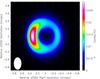 |
Fig. 3 ALMA simulated images at 345 GHz with an observation time of 2 h. The total flux of the source is 0.13 Jy and the contour lines are at 2, 4, 6, and 8 times the rms of 0.22 mJy. |
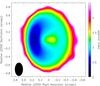 |
Fig. 4 Spectral index αmm using simulated images at bands 7 and 9. The antenna configuration was chosen such that the angular resolution is similar for both bands (~0.16′′, 22 AU at 140 pc). |
4. Summary and conclusions
We have shown that weak, but long-lived azimuthal asymmetries in the gas density can cause very efficient accumulation of dust
at the position of the azimuthal pressure maximum. We have derived analytical steady-state solutions for the dust distribution for any given azimuthal gas density distribution and the time scales on which these distributions develop. Good agreement has been found between the solutions and numerical simulations.
For this dust concentration mechanism to work, particles must grow to sufficiently large sizes (St > αt) such that the azimuthal drift becomes stronger than the turbulent diffusion. This typically corresponds to particles of sub-mm to cm sizes. The strong concentration of the largest grains leads to a size-sorting which is observable via low spectral indices at mm wavelengths and also in lopsided banana-shaped structures in resolved (sub-)mm images. Finding the size range where the bifurcation between concentration and diffusion happens would put constraints on the turbulence strength and the local gas density of the disk.
St = 1 typically corresponds to particles of mm to cm sizes in the outer disk. For typical disk conditions a ≃ 0.4 cm·St·Σg/1 g cm-2.
Acknowledgments
We thank Ewine van Dishoeck, Simon Bruderer, Nienke van der Marel, Geoffrey Mathews, Hui Li, and the referee for useful comments.
References
- Alexander, R. D., & Armitage, P. J. 2007, MNRAS, 375, 500 [NASA ADS] [CrossRef] [Google Scholar]
- Andrews, S. M., Wilner, D. J., Espaillat, C., et al. 2011, ApJ, 732, 42 [NASA ADS] [CrossRef] [Google Scholar]
- Barge, P., & Sommeria, J. 1995, A&A, 295, L1 [NASA ADS] [Google Scholar]
- Birnstiel, T., Dullemond, C. P., & Brauer, F. 2010, A&A, 513, A79 [NASA ADS] [CrossRef] [EDP Sciences] [Google Scholar]
- Birnstiel, T., Klahr, H., & Ercolano, B. 2012, A&A, 539, A148 [NASA ADS] [CrossRef] [EDP Sciences] [Google Scholar]
- Blum, J., & Wurm, G. 2008, ARA&A, 46, 21 [NASA ADS] [CrossRef] [EDP Sciences] [Google Scholar]
- Brauer, F., Dullemond, C. P., Johansen, A., et al. 2007, A&A, 469, 1169 [NASA ADS] [CrossRef] [EDP Sciences] [Google Scholar]
- Brauer, F., Henning, T., & Dullemond, C. P. 2008, A&A, 487, L1 [NASA ADS] [CrossRef] [EDP Sciences] [Google Scholar]
- Brown, J. M., Blake, G. A., Qi, C., Dullemond, C. P., & Wilner, D. J. 2008, ApJ, 675, L109 [NASA ADS] [CrossRef] [Google Scholar]
- Brown, J. M., Blake, G. A., Qi, C., et al. 2009, ApJ, 704, 496 [NASA ADS] [CrossRef] [Google Scholar]
- Cuzzi, J. N., & Hogan, R. C. 2003, Icarus, 164, 127 [NASA ADS] [CrossRef] [Google Scholar]
- Cuzzi, J. N., Hogan, R. C., & Shariff, K. 2008, ApJ, 687, 1432 [NASA ADS] [CrossRef] [Google Scholar]
- Dzyurkevich, N., Flock, M., Turner, N. J., Klahr, H., & Henning, T. 2010, A&A, 515, A70 [NASA ADS] [CrossRef] [EDP Sciences] [Google Scholar]
- Garaud, P. 2007, ApJ, 671, 2091 [NASA ADS] [CrossRef] [Google Scholar]
- Goldreich, P., & Ward, W. R. 1973, ApJ, 183, 1051 [NASA ADS] [CrossRef] [Google Scholar]
- Hughes, A. M., Andrews, S. M., Espaillat, C., et al. 2009, ApJ, 698, 131 [NASA ADS] [CrossRef] [Google Scholar]
- Isella, A., Natta, A., Wilner, D., Carpenter, J. M., & Testi, L. 2010, ApJ, 725, 1735 [NASA ADS] [CrossRef] [Google Scholar]
- Johansen, A., & Klahr, H. 2005, ApJ, 634, 1353 [NASA ADS] [CrossRef] [Google Scholar]
- Johansen, A., Oishi, J. S., Low, M.-M. M., et al. 2007, Nature, 448, 1022 [Google Scholar]
- Johansen, A., Youdin, A., & Klahr, H. 2009, ApJ, 697, 1269 [NASA ADS] [CrossRef] [Google Scholar]
- Klahr, H. H., & Henning, T. 1997, Icarus, 128, 213 [NASA ADS] [CrossRef] [Google Scholar]
- Kretke, K. A., & Lin, D. N. C. 2007, ApJ, 664, L55 [NASA ADS] [CrossRef] [Google Scholar]
- Lyra, W., Johansen, A., Klahr, H., & Piskunov, N. 2009, A&A, 493, 1125 [NASA ADS] [CrossRef] [EDP Sciences] [Google Scholar]
- Mayama, S., Hashimoto, J., Muto, T., et al. 2012, ApJ, 760, L26 [NASA ADS] [CrossRef] [Google Scholar]
- Meheut, H., Keppens, R., Casse, F., & Benz, W. 2012, A&A, 542, A9 [Google Scholar]
- Nakagawa, Y., Sekiya, M., & Hayashi, C. 1986, Icarus, 67, 375 [NASA ADS] [CrossRef] [Google Scholar]
- Natta, A., Testi, L., Neri, R., Shepherd, D. S., & Wilner, D. J. 2004, A&A, 416, 179 [NASA ADS] [CrossRef] [EDP Sciences] [Google Scholar]
- Okuzumi, S., Tanaka, H., Kobayashi, H., & Wada, K. 2012, ApJ, 752, 106 [NASA ADS] [CrossRef] [Google Scholar]
- Piétu, V., Dutrey, A., Guilloteau, S., Chapillon, E., & Pety, J. 2006, A&A, 460, L43 [NASA ADS] [CrossRef] [EDP Sciences] [Google Scholar]
- Pinilla, P., Benisty, M., & Birnstiel, T. 2012a, A&A, 545, A81 [NASA ADS] [CrossRef] [EDP Sciences] [Google Scholar]
- Pinilla, P., Birnstiel, T., Ricci, L., et al. 2012b, A&A, 538, A114 [NASA ADS] [CrossRef] [EDP Sciences] [Google Scholar]
- Regály, Z., Juhász, A., Sándor, Z., & Dullemond, C. P. 2012, MNRAS, 419, 1701 [NASA ADS] [CrossRef] [Google Scholar]
- Ricci, L., Testi, L., Natta, A., & Brooks, K. J. 2010a, A&A, 521, A66 [NASA ADS] [CrossRef] [EDP Sciences] [Google Scholar]
- Ricci, L., Testi, L., Natta, A., et al. 2010b, A&A, 512, A15 [NASA ADS] [CrossRef] [EDP Sciences] [Google Scholar]
- Rice, W. K. M., Armitage, P. J., Wood, K., & Lodato, G. 2006, MNRAS, 373, 1619 [NASA ADS] [CrossRef] [Google Scholar]
- Sándor, Z., Lyra, W., & Dullemond, C. P. 2011, ApJ, 728, L9 [NASA ADS] [CrossRef] [Google Scholar]
- Shakura, N. I., & Sunyaev, R. A. 1973, A&A, 24, 337 [NASA ADS] [Google Scholar]
- Testi, L., Natta, A., Shepherd, D. S., & Wilner, D. J. 2001, ApJ, 554, 1087 [Google Scholar]
- Testi, L., Natta, A., Shepherd, D. S., & Wilner, D. J. 2003, A&A, 403, 323 [NASA ADS] [CrossRef] [EDP Sciences] [Google Scholar]
- Weidenschilling, S. J. 1977, MNRAS, 180, 57 [NASA ADS] [CrossRef] [Google Scholar]
- Whipple, F. L. 1972, From Plasma to Planet, 211 [Google Scholar]
- Windmark, F., Birnstiel, T., Ormel, C. W., & Dullemond, C. P. 2012, A&A, 544, L16 [NASA ADS] [CrossRef] [EDP Sciences] [Google Scholar]
- Wolf, S., & Klahr, H. 2002, ApJ, 578, L79 [NASA ADS] [CrossRef] [Google Scholar]
- Youdin, A. N., & Lithwick, Y. 2007, Icarus, 192, 588 [NASA ADS] [CrossRef] [Google Scholar]
All Figures
|
Fig. 1 Contrast between the dust density in the azimuthal maximum and its surroundings for
different gas density contrasts ( |
| In the text | |
|
Fig. 2 Azimuthal steady-state solutions for small dust grains (red line) and large dust grains (blue line) for a given sinusoidal gas profile (black line, identical with red line). Dashed lines show numerical solutions at 1, 2, and 5 advection time scales. |
| In the text | |
|
Fig. 3 ALMA simulated images at 345 GHz with an observation time of 2 h. The total flux of the source is 0.13 Jy and the contour lines are at 2, 4, 6, and 8 times the rms of 0.22 mJy. |
| In the text | |
|
Fig. 4 Spectral index αmm using simulated images at bands 7 and 9. The antenna configuration was chosen such that the angular resolution is similar for both bands (~0.16′′, 22 AU at 140 pc). |
| In the text | |
Current usage metrics show cumulative count of Article Views (full-text article views including HTML views, PDF and ePub downloads, according to the available data) and Abstracts Views on Vision4Press platform.
Data correspond to usage on the plateform after 2015. The current usage metrics is available 48-96 hours after online publication and is updated daily on week days.
Initial download of the metrics may take a while.