| Issue |
A&A
Volume 550, February 2013
|
|
|---|---|---|
| Article Number | A102 | |
| Number of page(s) | 15 | |
| Section | Extragalactic astronomy | |
| DOI | https://doi.org/10.1051/0004-6361/201220710 | |
| Published online | 04 February 2013 | |
Anomalies in low-energy gamma-ray burst spectra with the Fermi Gamma-ray Burst Monitor
1
University College Dublin,
Belfield, Dublin 4,
Dublin,
Ireland
e-mail: This email address is being protected from spambots. You need JavaScript enabled to view it.
2
Physics Department, University of Alabama in
Huntsville, 320 Sparkman
Drive, Huntsville,
AL
35805,
USA
3
NASA Goddard Space Flight Center, Greenbelt, MD
20771,
USA
4
Institute for Astro and Particle Physics, University of
Innsbruck, Technikerstrasse
25, 6020
Innsbruck,
Austria
5
Max-Planck-Institut für extraterrestrische Physik,
Giessenbachstrasse 1,
85748
Garching,
Germany
6
Space Science Office, VP62, NASA/Marshall Space Flight
Center, Huntsville,
AL
35812,
USA
7
Exzellenz-Cluster Universe, Technische Universität
München, Boltzmannstrasse
2, 85748
Garching,
Germany
8
Science and Technology Institute, Universities Space Research
Association, 320 Sparkman
Drive, Huntsville,
AL
35805,
USA
Received: 8 November 2012
Accepted: 6 December 2012
Abstract
Context. A Band function has become the standard spectral function used to describe the prompt emission spectra of gamma-ray bursts (GRBs). However, deviations from this function have previously been observed in GRBs detected by BATSE and in individual GRBs from the Fermi era.
Aims. We present a systematic and rigorous search for spectral deviations from a Band function at low energies in a sample of the first two years of high fluence, long bursts detected by the Fermi Gamma-ray Burst Monitor (GBM). The sample contains 45 bursts with a fluence greater than 2 × 10⁻⁵ erg/cm2 (10−1000 keV).
Methods. An extrapolated fit method is used to search for low-energy spectral anomalies, whereby a Band function is fit above a variable low-energy threshold and then the best fit function is extrapolated to lower energy data. Deviations are quantified by examining residuals derived from the extrapolated function and the data and their significance is determined via comprehensive simulations which account for the instrument response. This method was employed for both time-integrated burst spectra and time-resolved bins defined by a signal-to-noise ratio of 25σ and 50σ.
Results. Significant deviations are evident in 3 bursts (GRB 081215A, GRB 090424 and GRB 090902B) in the time-integrated sample (~7%) and 5 bursts (GRB 090323, GRB 090424, GRB 090820, GRB 090902B and GRB 090926A) in the time-resolved sample (~11%).
Conclusions. The advantage of the systematic, blind search analysis is that it can demonstrate the requirement for an additional spectral component without any prior knowledge of the nature of that extra component. Deviations are found in a large fraction of high fluence GRBs; fainter GRBs may not have sufficient statistics for deviations to be found using this method.
Key words: gamma-ray burst: general / methods: data analysis / techniques: spectroscopic
© ESO, 2013
1. Introduction
Gamma-ray bursts (GRBs) are the most luminous events in the universe and can briefly be summarised as having high-energy prompt emission followed by a multi-wavelength fading afterglow (e.g., Vedrenne & Atteia 2009; Kann et al. 2011). The isotropic energy produced by a typical GRB is Eiso ~ 1051 erg (e.g., Frail et al. 2001) and in some cases reaches up to 1054 erg (e.g., Greiner et al. 2009; McBreen et al. 2010; Cenko et al. 2011). The prompt emission of GRBs has been detected over a wide spectral range from keV to GeV energies and is generally well modelled by one or a combination of the following: a smoothly broken power-law (e.g. Band et al. 1993; Abdo et al. 2009b), a quasi-thermal component (e.g., Preece 2000; Guiriec et al. 2011; Ryde et al. 2011; Axelsson et al. 2012), an extra non-thermal power-law component extending to high energies (e.g. González et al. 2003; Kaneko et al. 2008; Abdo et al. 2009a) or a cut-off in the MeV regime (e.g., Ackermann et al. 2012b). The lightcurves of GRBs are highly variable and a number of studies into their temporal properties have been performed (e.g., Quilligan et al. 2002; Hakkila & Preece 2011; Bhat et al. 2012).
Our work assumes that a Band function (Band et al. 1993) is the best fit function for GRB spectra in the GBM energy range and attempts to quantify the number of bursts that deviate from this function. In general, a Band function can be constrained better at lower energies compared to higher energies as more counts are observed at lower energies. This provides strict limits on the α parameter and makes it possible to search for deviations to the fit function. The Band model is defined as 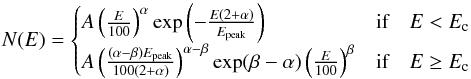 (1)where
 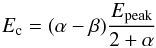 (2)and A is the amplitude in photons s-1 cm-2 keV-1, α is the low-energy power-law index, Epeak is the ν Fν peak energy in keV and β is the high-energy power-law index.
The emission mechanisms for GRBs have generally been described as thermal or non-thermal with the thermal emission characterised by the radiation emitted from a cooling plasma (e.g. Mészáros & Rees 2000). However, thermal emission need not take the form of a standard Planckian model but may take a more complex form depending on several factors including the relative leptonic and hadronic populations, viewing angles and source region (e.g., Ryde et al. 2011). Non-thermal emission can take the form of synchrotron emission from the extreme magnetic fields needed to create a GRB (e.g. Mészáros 2002). Strong magnetic fields may also break and reconnect releasing energy in the form of gamma-ray photons (e.g. Zhang & Yan 2011). Although a Band function is not a physical model, it successfully models a large number of GRBs and it is useful to investigate the number of events which require additional paramaters. If an additional blackbody is observed, the temperature of the photosphere can be deduced (Rees & Mészáros 2005) whereas an underlying power-law can provide constraints on emission mechanisms (e.g. Asano et al. 2009; Ryde et al. 2010) and the extragalactic background light (EBL, Ackermann et al. 2011). An overview of the observational and physical interpretations of the results from the Fermi era are presented by Bhat & Guiriec (2011).
A number of papers discuss interesting bursts with unusual spectral behaviour in the keV range (e.g., Guiriec et al. 2011; Ryde et al. 2011; Axelsson et al. 2012). It is important to note that there is a bias in the literature whereby interesting bursts are published more than bursts that conform to the standard GRB models. Another bias that can skew the apparent number of interesting bursts is that only bursts that look atypical initially are investigated further. A rigorous investigation must be carried out on a sample of GRBs in a systematic way to obtain the true fraction of GRBs with observable additional features. Any investigation must also be performed blindly to decrease the risk of interval selection effects which could bias the study. Here we present a systematic search for deviations from a Band function in the highest fluence bursts in the first catalogs from the Fermi Gamma-ray Burst Monitor (Paciesas et al. 2012; Goldstein et al. 2012).
1.1. Fermi Gamma-ray Burst Monitor
The Fermi Gamma-ray Space Telescope, launched on 2008 June 11, has an energy range spanning several decades (~8 keV to ~300 GeV) and is ideal to explore the low-energy regime of GRBs. Fermi consists of two instruments, the Large Area Telescope (LAT) operating between ~20 MeV to ~300 GeV (Atwood et al. 2009) and the Gamma-Ray Burst Monitor (GBM) operating between 8 keV−40 MeV (Meegan et al. 2009).
GBM consists of two types of detectors – twelve Sodium Iodide (NaI) scintillating crystals operating between 8−1000 keV and two Bismuth Germanate (BGO) scintillating crystals operating between 0.15−40 MeV. The NaI detectors are arranged in clusters of three around the edges of the satellite and the BGOs are located on opposing sides of the satellite aligned perpendicular to the LAT boresight. As the detectors have no active shield and are uncollimated, GBM observes the entire unocculted sky. Further details can be found in Meegan et al. (2009).
Both NaI and BGO detectors collect counts in 4096 channels compressed into 128 energy channels, with boundaries spaced pseudo-logarithmically across the energy ranges of each detector. The lowest and highest energy channels in each detector are generally ignored in the analysis because of uncertainties in the instrument response. Extensive ground calibration was carried out on the detectors pre-launch (Bissaldi et al. 2009) and in flight by comparison to other instruments (INTEGRAL-ISGRI: Tierney et al. 2011, INTEGRAL-SPI: von Kienlin et al. 2009 and Swift-BAT: Stamatikos 2009). These calibration results are consistent and do not show any major changes from the on-ground calibration. Additional calibration work has also been carried out using the Crab Nebula with Earth occultation techniques (Wilson-Hodge et al. 2012), nuclear lines from solar flares (Ackermann et al. 2012a), positron/electron annihilation lines (Briggs et al. 2011) and spectral analysis of soft gamma-ray repeaters (SGRs, Lin et al. 2012).
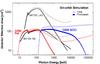 |
Fig. 1 Plot comparing the effective areas of GBM v BATSE per detector. The total area exposed to a particular sky direction depends on the orientation of each detector and number of detectors exposed. At low energies the GBM NaI detectors have more effective area than the BATSE SDs and at high energies the GBM BGO detectors have more effective area that the BATSE LAD (Meegan et al. 2009). The dark lines represent the photopeak effective area where the detected energy is the same (within the energy resolution) as the incident energy and the lighter lines represent the total effective area which includes the photopeak plus the cases where the instrument detects only part of the incident photon energy. (A colour version of this figure is available in the online journal.) |
1.2. Fermi GBM and BATSE/CGRO comparison
A comprehensive study examining deviations at the lower end of the spectrum has not been carried out since Preece et al. (1996) investigated time-integrated GRB spectra using the spectroscopy detectors (SDs) on the Burst And Transient Source Experiment (BATSE) on board the Compton Gamma Ray Observatory (CGRO) (Gehrels et al. 1992). The results of this study showed that ~14% of a sample of 86 GRBs contained significant low-energy excesses; no significant deficits were observed in the sample. A comparison between the effective areas of BATSE and GBM is given in Fig. 1. The GBM NaI detectors are of similar specifications to the BATSE SDs (see Table 1). As the BATSE SD detectors were significantly thicker than the GBM NaI detectors, the BATSE SDs could detect higher energy photons than the GBM NaIs. This is compensated for on GBM by using the BGO detectors for high-energy constraints.
The relative effective areas for each detector are presented in Fig. 1 showing that in the crucial energy range of interest (below ~30 keV), the NaIs have a greater effective area than the SD detectors. Additionally, while Preece et al. (1996) only used a single SD detector, multiple NaI detectors were used in our analysis in all but 3 GRBs (see Sect. 2). GBM also has the advantage of greater effective area at higher energies using the BGOs. This provides better constraints on β and Epeak which help constrain the overall spectral model applied to the data.
Comparison of properties of the GBM NaIs with the BATSE SDs.
To probe the lower energies using the BATSE SDs, two data types were required. The first data type was the Spectroscopy Discriminator data channels (DISCSP) which contained four integral channels over the entire energy range ~5 keV−2 MeV (for the highest gain setting). The upper edge of the lowest data channel (DISCSP 1) was set to the lower-level discriminator (LLD) threshold of the Spectroscopy High-Energy Resolution Burst (SHERB) data (~10 keV for the highest gain setting). The SHERB data comprised 256 spectral energy channels between the LLD and ~2 MeV. By using a joint fit between the SHERB data and the single DISCSP1 data point, Preece et al. (1996) determined the deviation of this single data point to the model. GBM has the advantage of a single standard data type from low to high energies. This reduces the chance of any incongruity between data sets. The data type also has better spectral resolution in the region of interest (see Table 1) so trends in the data can be more easily distinguished. GBM also has the advantage of better source locations provided by other instruments such as Swift and the LAT which improves the ability to accurately model the instrument response. Out of the sample of GRBs analysed in this work, 47% have a sub-degree localisation.
2. Sample selection
The sample was drawn from the first 2 years of triggered GBM GRBs (14th July 2008−13th July 2010). Bursts above a fluence of 2 × 10⁻⁵ erg cm-2 (10−1000 keV) were selected so that the spectral parameters could be constrained in the fitting process (see however Sect. 3.5). This gave a sample of 45 bursts, which formed the brightest 9% of the 491 GRBs in the first GBM GRB catalog (Paciesas et al. 2012). In addition, 36 out of the 45 GRBs (80%) have significant emission in at least one BGO detector as defined by Bissaldi et al. (2011). Only NaI detectors with source angles less than 60° were used in the spectral analysis to limit the effect of the uncertainties in the off-axis detector response. Two or more NaIs were used for 42 out of the 45 GRBs. The brightest BGO detector was used in all cases to constrain the spectral model at high energies.
As the signal-to-noise ratio (S/N) in these bursts is quite high, the influence of background fluctuations has a less statistically significant effect during the spectral fitting process compared to weaker bursts. Individual detectors were checked for blockages whereby the source photons passed through part of the spacecraft before entering a detector. This can cause photons to be scattered to different energies and lower energy photons to be absorbed beyond the ability of the detector response matrices (DRMs) to accurately reconstruct the photons incident on the entire spacecraft. An automated tool was initially used to check for line of sight blockages between the GRB and a detector. Further manual analysis was performed to remove any additional blocked detectors. Detectors that are blocked have a noticable deficiency of low-energy counts which is not consistent with other detectors that have similar source angles. Detectors which were not blocked and had an acceptable source angle were defined as “good” and used in the subsequent analysis.
Figure 2 shows the spectral properties of this sub-sample (α and Epeak) relative to the overall GBM spectral catalog (Goldstein et al. 2012). The distributions show that the sub-sample selected here displays similar characteristics to the entire GBM spectral catalogue.
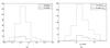 |
Fig. 2 Histograms comparing a) α and b) Epeak in the high fluence sample from our work to a sample obtained from Goldstein et al. (2012). |
3. Method
The sample was analysed using two methods. The first compares the data to the extrapolated fit of the function in the low-energy regime and the second compares the change in the spectral index α when the energy range of the data is shortened. These two methods are used in combination to identify deviations from a simple power-law at lower energies.
For an additional component to be significantly detected in the spectrum of a burst, it must either be continuously present throughout the entire burst or very strongly present in certain sections of the burst. An additional component may be present in certain sections of a GRB but not be intense enough to significantly alter the overall spectrum of the burst. Therefore the spectral fitting was performed on the spectrum of the entire burst (time-integrated) and on significant time slices (time-resolved) of the data. All spectral fitting was performed using the RMFIT software package1 and minor modifications were made to automate the fitting process.
3.1. Time-integrated single fit
CSPEC data were used for each “good” detector over the full energy range of GBM (8 keV−40 MeV). These data have an energy resolution of 128 channels and a temporal resolution of 4 s pre-trigger changing to 1 s post-trigger until T0 + 600 s. Using the lightcurve, a time region encompassing the main emission phase of the GRB was selected by eye. A polynomial background was then fit to each GRB lightcurve by selecting background regions before and after the prompt phase. Multiple response matrices were used in the fitting process to account for spacecraft slewing relative to the source. In this process a new response is made when the spacecraft slews by more than 2 degrees, which can be important in long bursts, and is especially important if the spacecraft executes an autonomous repoint. A similar method was also employed by Goldstein et al. (2012).
An initial time-integrated spectral fit was performed using a Band function for each GRB in the sample. Fit residuals were determined by the number of standard deviations that separate the data from a Band function. The residuals were summed between 8 keV and a variable low-energy threshold (LET) in order to search for excesses or deficits. The LET was set at 15, 20, 25, 30, 50 and 100 keV. However, this technique is not optimal as the fitting algorithm forces the function through any deviations that are present and minimises any deviations in any particular part of the spectrum. To reduce this issue, the LET was used as a lower energy bound for spectral fitting and the data points below the LET were compared to an extrapolated version of the function. This extrapolated fit is defined in the next section.
Although the sample was defined to be composed of high fluence GRBs, this does not necessarily guarantee a large number of counts in all energy channels. Due to the potential low count rate/bin ratio, the fit (minimization) was performed using Castor statistics. This is similar to Cash-statistics (Cash 1979). Castor statistics assume Poisson uncertainties per bin compared to χ2 statistics which assumes Gaussian uncertainties per bin. These are equivalent in the high count regime but diverge in the low count regime (less than ~10 counts/bin). A similar minimisation method was used by Goldstein et al. (2012).
3.2. Time-integrated extrapolated fit
An improved extrapolated fitting technique was devised such that a Band function was fit in the energy range from the variable LET to ~40 MeV. The function obtained from applying the model in this narrower range was then extrapolated to the lower energies in order to ascertain how well the function described the data below the LET. Deviations present between ~8 keV and the LET are quantified by summing the residuals between ~8 keV and the LET.
One of the assumptions of the extrapolated fitting technique is that the function parameters obtained over a shorter energy range should be consistent with a fit performed over the entire energy range in the absence of any spectral excesses or deficits with respect to the function. The parameters obtained by fitting from 8 keV−40 MeV should be consistent with those obtained by fitting from 15 keV−40 MeV when no additional components are present. The difference between the single fit method and extrapolated fit method is shown in Fig. 3. Minimizing C-stat will tend to produce a fit that balances excesses and deficits regardless of the physical origin of the deviation from a Band function. In the single fit method, the deviation at low energies results in strong fluctuations throughout the entire spectral energy range. When the extrapolated fit method is used, the spectral deviations are observed more clearly at lower energies and the effects on the remaining spectrum are reduced. Features in certain energy bands are not physically comparable between different GRBs because the energy bands are defined in the observer frame and redshifts are not known for all GRBs. However, when performing an analysis on the manifestation of observable deviations in certain energy bands, fits using the same LET can be compared using this method.
The low-energy power-law index, α, must be reasonably well constrained in order to confidently calculate the significance of any deviations. This implies that Epeak and the LET must be sufficiently different to ensure that α can be constrained over the shortened energy range. The technique also requires that Epeak is greater than the LET.
For each GRB, the spectral residuals between 8 keV and the LET are summed in an individual detector. The overall value for a particular GRB is the arithmetic mean for deviations in all detectors used in the analysis of the burst. The Iodine K-edge region of the spectrum around 33 keV can lead to larger residuals caused by systematics rather than a process intrinsic to the source. However, a strong K-edge effect was only noted in ~5 GRBs and dominated only 2 spectral bins. If the K-edge is present between 8 keV and the LET, it only weakly affects the summing of residuals over this range. In reality it is only relevant when LET = 50 or 100 keV and the effect was not deemed significant enough to alter the method.
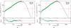 |
Fig. 3 Comparison of the single time-integrated fit to the extrapolated fitting technique. a) Single Band function fit to GRB 090902B from 8 keV−40 MeV ( |


3.3. Time-resolved extrapolated fit
The spectrum of a GRB can evolve over the prompt emission interval (e.g. Preece et al. 2000) and a time-resolved analysis is required to account for such evolution. An S/N approach was employed over a basic time-resolved analysis (i.e. splitting the bursts into time sections) to ensure significant counts per bin. The selected region for each GRB used in the time-integrated fitting (full burst) was binned to the 25σ and 50σ level above background in the brightest detector. These intervals were then used to define bins for all other detectors in a particular GRB. A fit was then performed on each newly defined bin.
3.4. Simulations
The goodness of fit of the data below the LET and the function fit at higher energies cannot easily be evaluated using C-Stat as there is no analytic result available to convert from the fit statistic to a measure of goodness of fit. Therefore it is difficult to quantify the significance of a deviation or even an acceptable range of values which occur in the absence of an excess/deficit at low energies. Simulations are therefore necessary to quantify whether a deviation is consistent with the extrapolated fit.
A boot-strapping method was used to compare the actual results from the data with simulated results. In order to perform the simulations, the background and source must be simulated. The background was simulated using a similar level to that in the real data. To obtain the source region, a perfect Band function specific to each GRB, or time interval selected, was simulated. Multiple count distributions were created using this function (varying by Poisson noise). Each set of parameters was simulated ~1000 times.
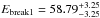
For each simulated spectrum, a distribution of low-energy deviations using different LETs can be compiled. The simulated distributions were then fit with a Gaussian distribution to obtain a value for the mean and standard deviation (see Fig. 5). The data obtained by summing the low-energy residuals below the LET were then normalised by calculating the number of standard deviations by which the data varied from the mean of the simulated distribution. If the data for a GRB differ significantly from its simulated distribution, then it is claimed that a low-energy deviation is present.
A representation of the overall distribution was simulated to provide an initial insight into the expected distribution of residuals assuming that all spectra were correctly described by a Band function. Five GRBs were selected from the sample which represented a broad range of peak energies, with Epeak = 161, 276, 444, 484 and 1010 keV. These GRBs were simulated and the resulting distribution of residuals in the absence of excesses/deficits are presented in Fig. 4. Individual simulations were then performed on a range of time-integrated and time-resolved sections of GRBs.
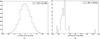 |
Fig. 4 Comparing the time-integrated data to a simulated distribution. a) Combined distribution of low-energy deviations of 5 individual GRBs assuming a perfect Band function (no deviations present). The extrapolated fit method was used with LET = 25 keV. b) The low-energy residuals of the GRBs in the sample that survived the data cuts (see Sect. 3.5) for LET = 25 keV. The data distribution b) is broadly similar to the simulated distribution a). The data point outside the main data distribution (on the right) is GRB 090902B. |
3.5. Data cuts
Several cuts were applied to the data before analysis. If any fit failed in the automated fitting process due to a lack of spectral constraints, it was excluded from the sample. A range of initial parameters were passed to the fitting process in order to obtain a satisfactory solution, but 9 fits failed in the time-resolved fitting process despite alternative initial parameters and were excluded from the sample. These fits were individually examined and the failure was usually due to low Epeak and a lack of counts above Epeak. No fits failed in the time-integrated analysis.
As the low-energy spectral index α only approaches a power-law in the asymptotic limit, a sufficient data range is needed to obtain reasonable constraints on the index. If Epeak is too close to the LET, two issues may arise 1) α will not approach the limit and 2) there will not be sufficient data to constrain α resulting in large fluctuations (e.g. LET = 50 keV, Epeak = 60 keV). A well constrained α parameter is required because slight variations in α can cause large spectral deviations when extrapolated to lower energies. For a spectrum to be accepted in the sample the following criteria must be met:
-
For LET = 15, 20, 25, 30 keV, Epeak > 100 keV is required.
-
For LETs = 50 or 100 keV, Epeak > 200 keV is required.
-
All intervals with a large proportional error on Epeak, Δ Epeak/Epeak > 0.45 were excluded.
-
All intervals with an error on α > 0.2 were discarded to ensure that α can be reasonably extrapolated beyond the range of the fit.
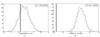 |
Fig. 5 Histograms of summed residuals below 25 keV obtained from time-integrated simulations of a perfect Band function. The dark line shows the value of the data for that GRB. a) The value of the deviation for GRB 080817A is − 3.6. The mean and the standard deviation of the simulated distribution are − 1.1 and 3.4 respectively. In this case the data does not deviate significantly from the simulated distribution and has a normalised deviation of − 0.7σ. b) The value of the deviation for GRB 090424 is − 25.8 compared to the simulated distribution with a mean and standard deviation of 0.4 and 4.3 respectively. The data deviates significantly from the simulated distribution with a normalised deviation of − 6.1σ. |
3.6. Variance of α
Another indication that a time interval in a burst had a low-energy spectral deviation was a variation in α when only the LET is changed. For each time section, each α parameter obtained from using different LETs was compared. If the value of α remains consistent across all different LETs in a spectrum, it is assumed that no significant low-energy deviations are present. If variation in α of > 2 σ for different LETs was evident, the GRB was investigated further. Usually a burst with a strong deviation in α would vary across multiple different LETs. If an interval had a variation in α and there was a deviation present in the low-energy residuals, this interval was concluded to have a significant spectral deviation from a Band function. All GRBs that had large deviations in the low-energy residuals displayed the expected variations in α.
3.7. Summary of method
A brief summary of the method for time-resolved analysis is presented below.
-
1.
The highest fluence GRBs from the first 2 years were selected for analysis.
-
2.
For each burst, NaI detectors <60° to the source and without blockages were selected. Multiple NaIs and a single BGO were selected in most cases.
-
3.
Background and source regions were selected for an individual burst.
-
4.
The main emission (time-integrated) interval of the GRB was selected by eye.
-
5.
The GRBs were binned by S/N over the time-integrated interval of the GRB to produce the time-resolved intervals.
-
6.
The individually significant S/N bins were then fit with a Band function from a LET to ~40 MeV.
-
7.
The LETs were selected to be 15, 20, 25, 30, 50, 100 keV.
-
8.
The fit function was then extrapolated to 8 keV.
-
9.
The residuals were summed between 8 keV and the LET for each detector and averaged across detectors.
-
10.
Simulations were then run and fit with a Gaussian distribution.
-
11.
The significance of deviations in the data were then quantified by the number of standard deviations by which the data varied from the mean of the simulated distribution.
-
12.
The α parameters between different LETs for a time region were compared.
-
13.
If a time region had a significant residual deviation and a variation in α while only changing the LET, it was considered to be a spectral deviation.
Number of sample GRBs / GRB intervals pre- and post-cuts.
4. Results
In the context of this work, spectral deviations can be classified into two broad categories – excesses and deficits. The former occur when there is an excess of photons with respect to the extrapolated fit function below the LET. These, for example, could be explained by an additional component such as a power-law or blackbody dominating at low energies. Deficits occur, not due to a lack of photons at low energies but because α is flatter than the actual data at low energies. This can be caused by the presence of an additional component, such as a blackbody, between the LET and Epeak resulting in a shallower α and a deficit of photons relative to the extrapolated function at low energies.
4.1. Hypothesis testing
Two methods were used to test for deviations at low energies. The first involves comparing the residuals from the data to those from simulations where a Band function is the assumed best fit. The results in Fig. 5 show two GRBs, one with and one without deviations using the time-integrated results. The null hypothesis for these simulations is that if the data are consistent with the simulated distribution, the extrapolated spectrum is consistent with a Band function.
The second method involves looking at the variation in α while only changing the LET for the time-resolved analysis. The changes in α for one GRB which is consistent with a Band function and one which is not consistent are presented in Fig. 6. Two GRBs, GRB 090618 and GRB 091024 showed variations in α but did not have large deviations in the low-energy residuals. The parameter α varied outside 2σ during one temporal interval for each of the GRBs. These intervals were investigated further and were discounted due to a long, weak interval in GRB 091024 and only having a single “good” detector available for analysis in GRB 090618.
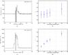 |
Fig. 6 Change in α between different LETs. The S/N temporal selections in GRB 090102 and GRB 090902B are presented in a) and c). The spectral parameter α is presented with 2σ error bars in b) and d) for LET values from 15 keV to 50 keV. α is consistent at the 2σ level as the LET is varied for the time interval selected in GRB 090102 and is not consistent for the time interval in GRB 090902B. |
Simulations were performed for GRBs that initially presented strong deviations in the time-integrated results. These deviations were then quantified by comparing the data to the simulated distribution for that GRB and were discarded as a chance occurrence if consistent with the simulations. Otherwise it was classified as a spectral deviation. A sample of GRBs were simulated that did not show strong deviations to ensure the veracity of the null hypothesis.
Simulations could not be performed for time-resolved regions of all GRBs so the combination of the two methods outlined previously (summing the low-energy residuals and checking the change in α between different LETs) present the final criterion by which a deviation is tested. If a deviation passed both tests then it was classified as a real spectral anomaly.
4.2. Time-integrated spectra
Out of the sample of 45 GRBs tested, a significant deviation in the time-integrated results was found in 3 cases GRB 090902B (T0+0 – T0+25 s), GRB 090424 (T0+0 – T0+6.4 s), GRB 081215A (T0+0 – T0+8.4 s). A large 28.2σ excess (normalised) is noted in GRB 090902B and is a clear outlier in Fig. 4. GRB 090424 has a deficit of 6.1σ in the time-integrated spectrum which appears to be due to an anomalous spectral feature near Epeak. These two GRBs also show deviations in the time-resolved spectral analysis. GRB 081215A manifests as a 6.7σ deficit but does not show up significantly in the time-resolved analysis. This deficit appears to be caused by strong spectral evolution throughout the GRB with Epeak decreasing from >1 MeV in the first 1 s time bin to ~50 keV at the end of the 8 s emission region (a time-resolved analysis by Zhang et al. (2011) using different binning shows similar results).
GRB 090902B may be fit with an intense additional power-law component throughout the entire burst causing it to deviate strongly in the time-integrated spectrum (Abdo et al. 2009a; Zhang et al. 2011). GRB 090424 has an intense additional component, which can be modelled as a blackbody throughout the burst which also manifests as a deviation in the time-integrated results. Additional emission processes and components may always be present in all GRBs but the instrument may not be sensitive enough to confidently detect them. A closer inspection of each GRB using time-resolved analysis is required to differentiate between artifacts in the spectra and real additional time-dependent spectral features.
4.3. Time-resolved spectra
A time-resolved analysis was performed on 672 spectra with an S/N of 25σ and 309 spectra with an S/N of 50σ which resulted in significant features in five bursts. GRB 090323, GRB 090424, GRB 090820, GRB 090902B and GRB 090926A contained at least one temporal interval where significant deviations were detected. Simulations were performed on the relevant time regions to ensure that they were significant. The properties of the five bursts are presented in Table 3.
Properties of the GRBs found to have strong spectral deviations in the time-resolved analysis at low energies.
Time-resolved spectral parameters from model fits to GRB time intervals where significant deviations were detected.
Out of the five bursts observed with low-energy deviations, four are in the top five most fluent GRBs from the first 2 years. In the case of the highest fluence event (GRB 090618 with a fluence of 2.68 × 10⁻⁴ ± 4.29 × 10⁻⁷ erg/cm2Paciesas et al. 2012), only one NaI was available for analysis due to the source-instrument geometry. It cannot be claimed with certainty that the result is stable on the basis of one “good” NaI detector. An analysis of this burst with the combined GBM-Swift data did not significantly demonstrate the need for an additional component in the prompt gamma-ray emission (Page et al. 2011).
As spectral evolution can lead to anomalous behaviour, even in the time-resolved analysis, lightcurves were examined for any notable features during a time interval which contained a deviation. To limit the effect of temporal binning, several further fits were performed by changing the length of the interval by up to ±50% and by shifting the interval up to 50%. If the effects were still significant after this further analysis it is claimed as a detection of an additional spectral feature. These intervals were then fit with more complex models and the results are summarised in Table 4. There is a notable improvement in the fit statistic when a Band function is fit with an additional component. This provides evidence that additional spectral features are needed to accurately model these time intervals. These solutions however are not unique and other spectral models may have a similar or better fit statistic.
4.4. Individual bursts with anomalous low-energy spectra
Significant anomalous spectral behaviour with respect to a Band function was found in time intervals of five bursts. The spectra were further investigated by fitting a number of spectral models as presented in Table 4. The individual events are described in more detail below.
4.4.1. GRB 090323
GRB 090323 was detected by Fermi GBM (van der Horst & Xin 2009) and LAT which caused the satellite to perform an autonomous repoint to the source location (Ohno et al. 2009). The lightcurve from GBM NaI detector n9 is displayed in Fig. 7 and consists of multiple distinct pulses over ~150 s. Multi-wavelength observations were aided by an on-ground location provided by the LAT and X-ray observations from Swift-XRT (Kennea et al. 2009). Follow-up observations report a spectroscopic redshift of z = 3.57 (Chornock et al. 2009a) and the afterglow was also detected at radio wavelengths (Harrison et al. 2009). The energetics and host galaxy properties of this burst are described in McBreen et al. (2010).
After performing a spectral analysis on this burst an excess is detected in two out of nine intervals (52−60 s, 60−66 s relative the trigger time). The spectral analysis for the interval with the strongest low-energy deviation is presented in Fig. 7 and Table 4. An improvement in the spectral residuals is notable when a Band + blackbody or Band + power-law fit is performed over a single Band fit.
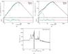 |
Fig. 7 Spectral fits for GRB 090323. a) A Band spectral fit and b) a Band + blackbody spectral fit are displayed for the hatched region of interest in c) the CSPEC lightcurve. All fits were performed on the full resolution data and the data were binned for illustrative purposes. The fit parameters are given in Table 4. |
4.4.2. GRB 090424
The prompt emission from GRB 090424 was detected by Swift-BAT, XRT and UVOT which provided an arcsecond localisation to the follow-up community within minutes (Cannizzo et al. 2009). The prompt emission was also observed by Fermi GBM (Connaughton 2009a) and Suzaku WAM (Hanabata et al. 2009). Multiple optical telescopes observed the optical afterglow (e.g. (Olivares et al. 2009b)) and a spectroscopic redshift of z = 0.544 was obtained by Gemini-South (Chornock et al. 2009b). Radio observations detected a bright radio afterglow (Chandra & Frail 2009) and a disturbance in Earth’s ionosphere was detected by monitoring very low frequency radio waves (Mondal et al. 2011; Chakrabarti et al. 2010).
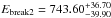
The main emission period of this GRB is relatively short compared to other bursts in the high fluence sample and has an extremely high peak flux of 110 photons/s (Paciesas et al. 2012). The burst has at least 3 pulses in rapid succession lasting ~6 s and lower level emission that continues up to 20 s after the trigger time. A significant low-energy deficit was observed in the time-integrated and time-resolved spectral analysis of GRB 090424. This apparent deficit is caused by the unusual spectral shape, which is shown in Fig. 8. The spectrum has 2 distinct spectral breaks, one in the usual energy range where a break due to Epeak is to be expected but also another lower energy break in the spectrum. A Band + blackbody fit with a blackbody kT of ~9 keV can be fit throughout the burst which is most prominent between 2−3 s relative to the trigger time. Six 1 s intervals between 0−6 s were analysed and a strong deviation is present in the residuals in the the 2−3 s region. Little spectral evolution is present throughout the burst, and as this feature is observable throughout the burst it is less likely to be caused by spectral evolution.
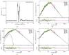 |
Fig. 8 Spectal fits for GRB 090424. a) The high-time resolution lightcurve of GRB 090424 with the hatched region being the region of interest. b) A simple Band fit to selected region. c) A Band + blackbody fit to the data. d) A double broken power-law fit with parameters of |


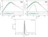 |
Fig. 9 Spectral data for GRB 090820. The data were fit with a) a Band function and b) a Band + blackbody function. c) The CSPEC lightcurve of GRB 090820 with the hatched region being the region of interest. |
4.4.3. GRB 090820
GBM detected GRB 090820 and issued an automated repoint request to Fermi, however the LAT could not observe the burst due to Earth avoidance constraints (Connaughton 2009b). The RT-2 Experiment onboard the CORONAS-PHOTON satellite also observed the prompt emission (Chakrabarti et al. 2009). No further follow-up of the burst occurred and thus the best location for the burst is obtained from GBM. The burst triggered on a weak precursor which was excluded from the spectral analysis.
This burst presents a low-energy deficit relative to a Band function which is caused by the Band function attempting to fit data that has a broader peak relative to the expected function fit. Thirteen time intervals between 29−45 s from the trigger time were analysed with five 1 s intervals between 31−36 s exhibiting marginal evidence of deviations. As this was the only GRB with consecutive marginal evidence for deviations, these time intervals were analysed together and display a strong deviation in the spectral data. By adding a blackbody component the Band function can account for the broader spectral peak as shown in Fig. 9. As an additional power-law could not account for deviations at lower energies, this provides evidence that some additional spectral property is occurring in the mid-energy range. Spectral analysis comparing standard models to more advanced fitting techniques, such as synchrotron models have been carried out by Burgess et al. (2011) for this burst.
4.4.4. GRB 090902B
GRB 090902B (Bissaldi & Connaughton 2009) was an extremely bright GRB with a bright additional component observed across 8 orders of magnitude in energy (Abdo et al. 2009a). The GRB was initially detected by both instruments on Fermi, GBM and the LAT (Bissaldi & Connaughton 2009; de Palma et al. 2009). The prompt emission was also detected by Suzaku WAM (Terada et al. 2009). A Target of Opportunity (ToO) was issued to Swift which observed an uncataloged source within the LAT error radius (Kennea & Stratta 2009). Numerous optical follow-up observations were made (e.g. Olivares et al. 2009a) resulting in a redshift of z = 1.822 (Cucchiara et al. 2009). The source was also observed in the radio (van der Horst et al. 2009).
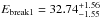
A significant excess was observed in this GRB in numerous intervals (ten 1-second intervals between 6−16 s relative the trigger time). The region with the stongest deviation is presented in Table 4. An additional power-law component was the best fit model to the data out of the models tested. The additional power-law index from analysing the GBM data only in this region,  , is consistent with the power-law index observed by a joint fit over the entire spectral range of GBM and LAT (
 ). Complex spectral models to this GRB are fit in Fig. 10. Numerous models have been presented in the literature to explain the spectral features in this burst (Liu & Wang 2011; Barniol Duran & Kumar 2011; Pe’er et al. 2012).
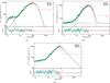 |
Fig. 10 Spectral fits applied to the the time interval of T0+9.7 – T0+10.6 s for GRB 090902B. Fits performed to decribe the data include; a) a Band + blackbody fit, b) Band + power-law fit and c) a double broken power-law fit with parameters of |


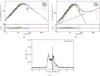 |
Fig. 11 Spectral fitting of GRB 090926A. The data were fit with a) a Band function and b) a Band + power-law model. A high-resolution lightcurve is displayed in c) to highlight the short sharp spike in the data. |
4.4.5. GRB 090926A
Detected by GBM (Bissaldi 2009) and LAT (Uehara et al. 2009), follow-up observations of this GRB were made by Swift-XRT (Vetere et al. 2009) and Swift-UVOT (Gronwall & Vetere 2009). The prompt emission was also observed by Suzaku WAM (Noda et al. 2009) and Konus-Wind (Golenetskii et al. 2009). A redshift of z = 2.1062 was obtained by the Very Large Telescope (VLT) X-Shooter spectrograph (Malesani et al. 2009). Skynet/PROMPT also observed the optical afterglow (Haislip et al. 2009).
GRB 090926A has also been observed in joint GBM and LAT spectral fitting to necessitate an additional power-law component over a wide spectral range (Ackermann et al. 2011). Thirteen time bins were analysed between 0−17 s with one time bin showing a significant excess. The excess is observed during a short sharp spike in the lightcurve which is shown in Fig. 11. When an additional power-law is fit with a Band function, the fit statistic shows a large improvement. The additional power-law index  , obtained by using GBM data only, is again consistent with the power-law observed in the LAT at high energies
  (Ackermann et al. 2011).
5. Discussion and conclusions
Although an empirical model, a Band function has been used to model the majority of GRB spectra since it was first proposed in 1993 (Band et al. 1993). However recent GRB studies with Fermi have suggested that there are a number of GRBs whose spectral behaviour differs from a Band function, with a number of different spectral components invoked in order to explain these observations (e.g. Asano et al. 2009; Burgess et al. 2011; Guiriec et al. 2011; Pe’er et al. 2012). The Fermi data cover a wide energy band with high spectral resolution and so the systematic study of low-energy spectral deviations in bright Fermi bursts presented here enables the frequency of such events to be investigated. Spectral deviations to a Band function occurring throughout the GBM energy range also affect the spectrum at low energies, and so the current method provides a systematic study over the full GBM energy range, assuming that the spectral data are adequately modelled by a Band function.
GBM observes 3 out of 45 (~7%) GRBs with spectral deviations present in the time-integrated data. The probability that our observed rate is consistent with the BATSE observed rate is ~7.0% or within 1.8σ. An excess is observed in one GRB (GRB 090902B) and deficits are observed in two (GRB 090424 and GRB 081215A) in the time-integrated data, while BATSE observed only excesses at low energies. There are a number of possible causes for the differences between the results obtained from the two instruments. As described in Sect. 1.2, the study of low-energy GRB spectra with BATSE was performed using two data types from two different SDs, with the observations depending on a single DISCSP1 data point at low energies. The structure of these datatypes mean that the low and high-energy bounds of the DISCSP1 point can vary from one GRB to another. GBM has the advantage of a single data type with high spectral resolution over its full energy range allowing deviations to be investigated in fixed energy ranges. Multiple GBM detectors were also used for this analysis, with GRBs having only one ‘good’ detector being analysed for 3 out of 45 GRBs. The effective areas of both instruments are also different. The DRMs of the GBM GRBs are well defined due to their small source location uncertainties, with 80% of the GRBs with spectral deviations having Swift-XRT locations. It is therefore difficult to make a direct comparison between the GBM and BATSE results. For the reasons outlined above we consider that the GBM result is more robust.
Since spectral evolution throughout the duration of a GRB significantly affects the spectral shape, a time-resolved analysis was performed for all of the GRBs in the sample. Spectral deviations are found in 11% of the GRBs in at least one time interval by applying the methods outlined in this paper. Our work shows that the features in the spectra are time-dependent and a time-resolved analysis is necessary to limit the effects of averaging multiple spectra. It is interesting to note that 4 of the 5 GRBs with significant features in the time-resolved analysis are in the top 5 most fluent GRBs in the sample. A bias exists whereby additional models are more likely to be required in high fluence GRBs since these GRBs have enough statistics to confidently define an additional component, if present.
The observed deviations may be due to significant spectral evolution in the burst (or time interval) or additional spectral features/components in the spectrum. In the time-integrated analysis, the deviation found in GRB 081215A may be due to spectral evolution, while the deviations in GRB 090424 and GRB 090902B could be explained by additional spectral features. For those GRBs with deviations found in shorter time intervals (GRB 090902B and GRB 090926A), a power-law improves the fit at lower energies which is consistent with the high-energy observations in the LAT data (Abdo et al. 2009a; Ackermann et al. 2011). For GRB 090424 and GRB 090820 an additional blackbody component provides a significantly better fit to the data than an additional power-law, showing that a number of different spectral components may be present in GRBs. GRB 090323 is adequately fit invoking either of the two additional components. However as there is little evidence for LAT emission (Piron et al. 2011), it is unlikely to be due to an additional power-law component extending to high energies and a spectral cut-off between the GBM and LAT energy bands is possible.
The advantage of the method presented in this paper is that it can demonstrate the requirement for an additional spectral component with respect to a Band function without any prior knowledge of the nature of that extra component. Theoretical models of the GRB emission process must be able to explain why the majority of GRBs are adequately modelled by a Band function and also explain the observed deviations. Many physical models have recently been proposed (see Sect. 1), however in many cases the spectral data do not have adequate statistics for one model to be deemed more statistically significant than another.
This technique demonstrates a systematic method to search GRBs for additional components at low-energies. The method finds several GRBs in which features have previously been noted as well as discovering deviations in GRB 090424 and GRB 090323. Deviations are found in a large fraction of high fluence GRBs; this method may be unable to find low-energy deviations in fainter GRBs. This suggests that deviations from a Band function may be common in all GRBs but the statistics do not allow us to test this hypothesis.
Acknowledgments
D.T. acknowledges support from Science Foundation Ireland under grant number 09-RFP-AST-2400. G.F. acknowledges the support of the Irish Research Council. S.F. acknowledges the support of the Irish Research Council for Science, Engineering and Technology, cofunded by Marie Curie Actions under FP7. S.G. was supported by the NASA Postdoctoral Program (NPP) at the NASA/Goddard Space Flight Center, administered by Oak Ridge Associated Universities through a contract with NASA. S.G. acknowledges financial support through the Cycle-4 NASA Fermi Guest Investigator program. A.v.K. acknowledges support by the German Aerospace Center, through DLR 50 QV 0301.
References
- Abdo, A. A., Ackermann, M., Ajello, M., et al. 2009a, ApJ, 706, L138 [NASA ADS] [CrossRef] [Google Scholar]
- Abdo, A. A., Ackermann, M., Arimoto, M., et al. 2009b, Science, 323, 1688 [Google Scholar]
- Ackermann, M., Ajello, M., Asano, K., et al. 2011, ApJ, 729, 114 [CrossRef] [Google Scholar]
- Ackermann, M., Ajello, M., Allafort, A., et al. 2012a, ApJ, 748, 151 [NASA ADS] [CrossRef] [Google Scholar]
- Ackermann, M., Ajello, M., Baldini, L., et al. 2012b, ApJ, 754, 121 [NASA ADS] [CrossRef] [Google Scholar]
- Asano, K., Guiriec, S., & Mészáros, P. 2009, ApJ, 705, L191 [NASA ADS] [CrossRef] [Google Scholar]
- Atwood, W. B., Abdo, A. A., Ackermann, M., et al. 2009, ApJ, 697, 1071 [NASA ADS] [CrossRef] [Google Scholar]
- Axelsson, M., Baldini, L., Barbiellini, G., et al. 2012, ApJ, 757, L31 [NASA ADS] [CrossRef] [Google Scholar]
- Band, D., Matteson, J., Ford, L., et al. 1993, ApJ, 413, 281 [NASA ADS] [CrossRef] [Google Scholar]
- BarniolDuran, R., & Kumar, P. 2011, MNRAS, 417, 1584 [NASA ADS] [CrossRef] [Google Scholar]
- Bhat, P. N., & Guiriec, S. 2011, Bull. Astron. Soc. India, 39, 471 [NASA ADS] [Google Scholar]
- Bhat, P. N., Briggs, M. S., Connaughton, V., et al. 2012, ApJ, 744, 141 [NASA ADS] [CrossRef] [Google Scholar]
- Bissaldi, E. 2009, GRB Coordinates Network, 9933, 1 [NASA ADS] [Google Scholar]
- Bissaldi, E., & Connaughton, V. 2009, GRB Coordinates Network, 9866, 1 [NASA ADS] [Google Scholar]
- Bissaldi, E., von Kienlin, A., Lichti, G., et al. 2009, Exp. Astron., 24, 47 [NASA ADS] [CrossRef] [Google Scholar]
- Bissaldi, E., von Kienlin, A., Kouveliotou, C., et al. 2011, ApJ, 733, 97 [NASA ADS] [CrossRef] [Google Scholar]
- Briggs, M. S., Connaughton, V., Wilson-Hodge, C., et al. 2011, Geophys. Res. Lett., 38, L02808 [NASA ADS] [CrossRef] [Google Scholar]
- Burgess, J. M., Preece, R. D., Baring, M. G., et al. 2011, ApJ, 741, 24 [NASA ADS] [CrossRef] [Google Scholar]
- Cannizzo, J. K., Barthelmy, S. D., Beardmore, A. P., et al. 2009, GRB Coordinates Network, 9223, 1 [NASA ADS] [Google Scholar]
- Cash, W. 1979, ApJ, 228, 939 [NASA ADS] [CrossRef] [Google Scholar]
- Cenko, S. B., Frail, D. A., Harrison, F. A., et al. 2011, ApJ, 732, 29 [NASA ADS] [CrossRef] [Google Scholar]
- Chakrabarti, S. K., Nandi, A., Debnath, D., et al. 2009, GRB Coordinates Network, 9833, 1 [NASA ADS] [Google Scholar]
- Chakrabarti, S. K., Mandal, S. K., Sasmal, S., et al. 2010, Indian J. Phys., 84, 1461 [NASA ADS] [CrossRef] [Google Scholar]
- Chandra, P., & Frail, D. A. 2009, GRB Coordinates Network, 9260, 1 [NASA ADS] [Google Scholar]
- Chornock, R., Perley, D. A., Cenko, S. B., & Bloom, J. S. 2009a, GRB Coordinates Network, 9028, 1 [NASA ADS] [Google Scholar]
- Chornock, R., Perley, D. A., Cenko, S. B., & Bloom, J. S. 2009b, GRB Coordinates Network, 9243, 1 [NASA ADS] [Google Scholar]
- Connaughton, V. 2009a, GRB Coordinates Network, 9230, 1 [NASA ADS] [Google Scholar]
- Connaughton, V. 2009b, GRB Coordinates Network, 9829, 1 [NASA ADS] [Google Scholar]
- Cucchiara, A., Fox, D. B., Tanvir, N., & Berger, E. 2009, GRB Coordinates Network, 9873, 1 [NASA ADS] [Google Scholar]
- de Palma, F., Bregeon, J., & Tajima, H. 2009, GRB Coordinates Network, 9867, 1 [NASA ADS] [Google Scholar]
- Frail, D. A., Kulkarni, S. R., Sari, R., et al. 2001, ApJ, Lett., 562, L55 [Google Scholar]
- Gehrels, N., Kniffen, D. A., & Ormes, J. F. 1992, in Current Topics in Astrofundamental Physics, eds. N. Sanchez, & A. Zichichi, 602 [Google Scholar]
- Goldstein, A., Burgess, J. M., Preece, R. D., et al. 2012, ApJS, 199, 19 [NASA ADS] [CrossRef] [Google Scholar]
- Golenetskii, S., Aptekar, R., Mazets, E., et al. 2009, GRB Coordinates Network, 9959, 1 [NASA ADS] [Google Scholar]
- González, M. M., Dingus, B. L., Kaneko, Y., et al. 2003, Nature, 424, 749 [NASA ADS] [CrossRef] [PubMed] [Google Scholar]
- Greiner, J., Clemens, C., Krühler, T., et al. 2009, A&A, 498, 89 [NASA ADS] [CrossRef] [EDP Sciences] [Google Scholar]
- Gronwall, C., & Vetere, L. 2009, GRB Coordinates Network, 9938, 1 [NASA ADS] [Google Scholar]
- Guiriec, S., Connaughton, V., Briggs, M. S., et al. 2011, ApJ, 727, L33 [NASA ADS] [CrossRef] [Google Scholar]
- Haislip, J., Reichart, D., Ivarsen, K., et al. 2009, GRB Coordinates Network, 9937, 1 [NASA ADS] [Google Scholar]
- Hakkila, J., & Preece, R. D. 2011, ApJ, 740, 104 [NASA ADS] [CrossRef] [Google Scholar]
- Hanabata, Y., Uehara, T., Takahashi, T., et al. 2009, GRB Coordinates Network, 9270, 1 [NASA ADS] [Google Scholar]
- Harrison, F., Cenko, B., Frail, D. A., Chandra, P., & Kulkarni, S. 2009, GRB Coordinates Network, 9043, 1 [NASA ADS] [Google Scholar]
- Kaneko, Y., González, M. M., Preece, R. D., Dingus, B. L., & Briggs, M. S. 2008, ApJ, 677, 1168 [NASA ADS] [CrossRef] [Google Scholar]
- Kann, D. A., Klose, S., Zhang, B., et al. 2011, ApJ, 734, 96 [NASA ADS] [CrossRef] [Google Scholar]
- Kennea, J. A., & Stratta, G. 2009, GRB Coordinates Network, 9868, 1 [NASA ADS] [Google Scholar]
- Kennea, J., Evans, P., & Goad, M. 2009, GRB Coordinates Network, 9024, 1 [NASA ADS] [Google Scholar]
- Lin, L., Göğüş, E., Baring, M. G., et al. 2012, ApJ, 756, 54 [NASA ADS] [CrossRef] [Google Scholar]
- Liu, R.-Y., & Wang, X.-Y. 2011, ApJ, 730, 1 [NASA ADS] [CrossRef] [Google Scholar]
- Malesani, D., Goldoni, P., Fynbo, J. P. U., et al. 2009, GRB Coordinates Network, 9942, 1 [NASA ADS] [Google Scholar]
- McBreen, S., Krühler, T., Rau, A., et al. 2010, A&A, 516, A71 [NASA ADS] [CrossRef] [EDP Sciences] [Google Scholar]
- Meegan, C., Lichti, G., Bhat, P. N., et al. 2009, ApJ, 702, 791 [NASA ADS] [CrossRef] [Google Scholar]
- Mészáros, P. 2002, ARA&A, 40, 137 [NASA ADS] [CrossRef] [MathSciNet] [Google Scholar]
- Mészáros, P., & Rees, M. J. 2000, ApJ, 530, 292 [NASA ADS] [CrossRef] [Google Scholar]
- Mondal, S. K., Chakrabarti, S. K., Choudhury, A., Chatterjee, A., & Bhowmick, D. 2011, GRB Coordinates Network, 11883, 1 [Google Scholar]
- Noda, K., Sonoda, E., Ohmori, N., et al. 2009, GRB Coordinates Network, 9951, 1 [NASA ADS] [Google Scholar]
- Ohno, M., Cutini, S., McEnery, J., Chiang, J., & Koerding, E. 2009, GRB Coordinates Network, 9021, 1 [NASA ADS] [Google Scholar]
- Olivares, F., Afonso, P., Greiner, J., et al. 2009a, GRB Coordinates Network, 9874, 1 [NASA ADS] [Google Scholar]
- Olivares, F., Kupcu Yoldas, A., Greiner, J., & Yoldas, A. 2009b, GRB Coordinates Network, 9245, 1 [NASA ADS] [Google Scholar]
- Paciesas, W. S., Meegan, C. A., von Kienlin, A., et al. 2012, ApJS, 199, 18 [NASA ADS] [CrossRef] [Google Scholar]
- Page, K. L., Starling, R. L. C., Fitzpatrick, G., et al. 2011, MNRAS, 416, 2078 [NASA ADS] [CrossRef] [Google Scholar]
- Pe’er, A., Zhang, B.-B., Ryde, F., et al. 2012, MNRAS, 420, 468 [NASA ADS] [CrossRef] [Google Scholar]
- Piron, F., McEnery, J., & Vasileiou, V. 2011, in AIP Conf. Ser. 1358, eds. J. E. McEnery, J. L. Racusin, & N. Gehrels, 47 [Google Scholar]
- Preece, R. D. 2000, in AAS/High Energy Astrophysics Division #5, BAAS, 32, 1231 [Google Scholar]
- Preece, R. D., Briggs, M. S., Pendleton, G. N., et al. 1996, ApJ, 473, 310 [NASA ADS] [CrossRef] [Google Scholar]
- Preece, R. D., Briggs, M. S., Mallozzi, R. S., et al. 2000, ApJS, 126, 19 [NASA ADS] [CrossRef] [Google Scholar]
- Quilligan, F., McBreen, B., Hanlon, L., et al. 2002, A&A, 385, 377 [NASA ADS] [CrossRef] [EDP Sciences] [Google Scholar]
- Rees, M. J., & Mészáros, P. 2005, ApJ, 628, 847 [NASA ADS] [CrossRef] [Google Scholar]
- Ryde, F., Axelsson, M., Zhang, B. B., et al. 2010, ApJ, 709, L172 [NASA ADS] [CrossRef] [Google Scholar]
- Ryde, F., Pe’er, A., Nymark, T., et al. 2011, MNRAS, 415, 3693 [NASA ADS] [CrossRef] [Google Scholar]
- Stamatikos, M. 2009, ArXiv e-prints [Google Scholar]
- Terada, Y., Tashiro, M., Endo, A., et al. 2009, GRB Coordinates Network, 9897, 1 [NASA ADS] [Google Scholar]
- Tierney, D., McBreen, S., Hanlon, L., et al. 2011, in AIP Conf. Ser. 1358, eds. J. E. McEnery, J. L. Racusin, & N. Gehrels, 397 [Google Scholar]
- Uehara, T., Takahashi, H., & McEnery, J. 2009, GRB Coordinates Network, 9934, 1 [NASA ADS] [Google Scholar]
- van der Horst, A. J., & Xin, L. P. 2009, GRB Coordinates Network, 9035, 1 [NASA ADS] [Google Scholar]
- van der Horst, A. J., Kamble, A. P., Wijers, R. A. M. J., & Kouveliotou, C. 2009, GRB Coordinates Network, 9883, 1 [NASA ADS] [Google Scholar]
- Vedrenne, G., & Atteia, J. L. 2009, Gamma-Ray Bursts: The brightest explosions in the Universe (Springer Praxis Books, Astronomy and Planetary Sciences Jointly published with Praxis Publishing) [Google Scholar]
- Vetere, L., Evans, P. A., & Goad, M. R. 2009, GRB Coordinates Network, 9936, 1 [NASA ADS] [Google Scholar]
- von Kienlin, A., Briggs, M. S., Connoughton, V., et al. 2009, in AIP Conf. Ser. 1133, eds. C. Meegan, C. Kouveliotou, & N. Gehrels, 446 [Google Scholar]
- Wilson-Hodge, C. A., Case, G. L., Cherry, M. L., et al. 2012, ApJ, 201, 33 [Google Scholar]
- Zhang, B., & Yan, H. 2011, ApJ, 726, 90 [NASA ADS] [CrossRef] [Google Scholar]
- Zhang, B.-B., Zhang, B., Liang, E.-W., et al. 2011, ApJ, 730, 141 [NASA ADS] [CrossRef] [Google Scholar]
All Tables
Properties of the GRBs found to have strong spectral deviations in the time-resolved analysis at low energies.
Time-resolved spectral parameters from model fits to GRB time intervals where significant deviations were detected.
All Figures
|
Fig. 1 Plot comparing the effective areas of GBM v BATSE per detector. The total area exposed to a particular sky direction depends on the orientation of each detector and number of detectors exposed. At low energies the GBM NaI detectors have more effective area than the BATSE SDs and at high energies the GBM BGO detectors have more effective area that the BATSE LAD (Meegan et al. 2009). The dark lines represent the photopeak effective area where the detected energy is the same (within the energy resolution) as the incident energy and the lighter lines represent the total effective area which includes the photopeak plus the cases where the instrument detects only part of the incident photon energy. (A colour version of this figure is available in the online journal.) |
| In the text | |
|
Fig. 2 Histograms comparing a) α and b) Epeak in the high fluence sample from our work to a sample obtained from Goldstein et al. (2012). |
| In the text | |
|
Fig. 3 Comparison of the single time-integrated fit to the extrapolated fitting technique. a) Single Band function fit to GRB 090902B from 8 keV−40 MeV ( |
| In the text | |
|
Fig. 4 Comparing the time-integrated data to a simulated distribution. a) Combined distribution of low-energy deviations of 5 individual GRBs assuming a perfect Band function (no deviations present). The extrapolated fit method was used with LET = 25 keV. b) The low-energy residuals of the GRBs in the sample that survived the data cuts (see Sect. 3.5) for LET = 25 keV. The data distribution b) is broadly similar to the simulated distribution a). The data point outside the main data distribution (on the right) is GRB 090902B. |
| In the text | |
|
Fig. 5 Histograms of summed residuals below 25 keV obtained from time-integrated simulations of a perfect Band function. The dark line shows the value of the data for that GRB. a) The value of the deviation for GRB 080817A is − 3.6. The mean and the standard deviation of the simulated distribution are − 1.1 and 3.4 respectively. In this case the data does not deviate significantly from the simulated distribution and has a normalised deviation of − 0.7σ. b) The value of the deviation for GRB 090424 is − 25.8 compared to the simulated distribution with a mean and standard deviation of 0.4 and 4.3 respectively. The data deviates significantly from the simulated distribution with a normalised deviation of − 6.1σ. |
| In the text | |
|
Fig. 6 Change in α between different LETs. The S/N temporal selections in GRB 090102 and GRB 090902B are presented in a) and c). The spectral parameter α is presented with 2σ error bars in b) and d) for LET values from 15 keV to 50 keV. α is consistent at the 2σ level as the LET is varied for the time interval selected in GRB 090102 and is not consistent for the time interval in GRB 090902B. |
| In the text | |
|
Fig. 7 Spectral fits for GRB 090323. a) A Band spectral fit and b) a Band + blackbody spectral fit are displayed for the hatched region of interest in c) the CSPEC lightcurve. All fits were performed on the full resolution data and the data were binned for illustrative purposes. The fit parameters are given in Table 4. |
| In the text | |
|
Fig. 8 Spectal fits for GRB 090424. a) The high-time resolution lightcurve of GRB 090424 with the hatched region being the region of interest. b) A simple Band fit to selected region. c) A Band + blackbody fit to the data. d) A double broken power-law fit with parameters of |
| In the text | |
|
Fig. 9 Spectral data for GRB 090820. The data were fit with a) a Band function and b) a Band + blackbody function. c) The CSPEC lightcurve of GRB 090820 with the hatched region being the region of interest. |
| In the text | |
|
Fig. 10 Spectral fits applied to the the time interval of T0+9.7 – T0+10.6 s for GRB 090902B. Fits performed to decribe the data include; a) a Band + blackbody fit, b) Band + power-law fit and c) a double broken power-law fit with parameters of |
| In the text | |
|
Fig. 11 Spectral fitting of GRB 090926A. The data were fit with a) a Band function and b) a Band + power-law model. A high-resolution lightcurve is displayed in c) to highlight the short sharp spike in the data. |
| In the text | |
Current usage metrics show cumulative count of Article Views (full-text article views including HTML views, PDF and ePub downloads, according to the available data) and Abstracts Views on Vision4Press platform.
Data correspond to usage on the plateform after 2015. The current usage metrics is available 48-96 hours after online publication and is updated daily on week days.
Initial download of the metrics may take a while.