| Issue |
A&A
Volume 550, February 2013
|
|
|---|---|---|
| Article Number | A30 | |
| Number of page(s) | 8 | |
| Section | The Sun | |
| DOI | https://doi.org/10.1051/0004-6361/201220469 | |
| Published online | 21 January 2013 | |
Nanoflare statistics in an active region 3D MHD coronal model
Max Planck Institute for Solar System Research (MPS), 37191 Katlenburg-Lindau, Germany
e-mail: This email address is being protected from spambots. You need JavaScript enabled to view it.
; This email address is being protected from spambots. You need JavaScript enabled to view it.
Received: 30 September 2012
Accepted: 10 December 2012
Abstract
Aims. We investigate the statistics for the spatial and temporal distribution of the energy input into the corona in a three-dimensional magneto-hydrodynamical (3D MHD) model. The model describes the temporal evolution of the corona above an observed active region. The model is driven by photospheric granular motions that braid the magnetic field lines. This induces currents that are dissipated, thereby leading to transient heating of the coronal plasma. We evaluate the transient heating as subsequent heating events and analyze their statistics. The results are then interpreted in the context of observed flare statistics and coronal heating mechanisms. Observed solar flares and other smaller transients cover a wide range of energies. The frequency distribution of energies follow a power law, the lower end of the distribution given by the detection limit of current instrumentation. One particular heating mechanism is based on the occurrence of so-called nanoflares, i.e. very low-energy deposition events.
Methods. To conduct the numerical experiment we use a high-order finite-difference code that solves the partial differential equations for the conservation of mass, the momentum and energy balance, and the induction equation. The energy balance includes Spitzer heat conduction and optically thin radiative losses in the corona.
Results. The temporal and spatial distribution of the Ohmic heating in the 3D MHD model follows a power law and can therefore be understood as a system in a self-organized critical state. The slopes of the power law are similar to the results based on observations of flares and smaller transients. We find that the coronal heating is dominated by events similar to the so-called nanoflares with energies on the order of 1017 J or 1024 erg.
Key words: Sun: corona / stars: coronae / magnetohydrodynamics (MHD) / methods: numerical
© ESO, 2013
1. Introduction
In the upper atmosphere of the Sun and stars, energy is released in a transient fashion. Strong flares are just the tip of the iceberg, where the plasma can be heated up to 10 MK or more and particles are accelerated to relativistic speeds. More numerous are smaller energy releases that cause smaller brightenings in X-rays and extreme UV, down to the current detection limit. There is a continuous connection from these smallest observable brightenings, often called microflares, to the largest of flares in the sense that the distribution in energy of all these events roughly follows a power law. Theoretical arguments have been proposed that even smaller transient releases of energy have to exist, the nanoflares (Parker 1988), which could play a major role in the heating of the corona. In this study we investigate the energy distribution of these low energy releases as they are found in 3D magnetohydrodynamics (MHD) models.
Rosner & Vaiana (1978) have already investigated the transient events of the Sun, flaring stars, and other X-ray sources. They found that the energy distribution of these events roughly follows a power law. To explain the flare statistics Rosner & Vaiana (1978) provided a theoretical model that led to a power-law distribution of the flare parameters. This model was based on the assumptions that flaring is a stochastic relaxation, the waiting time between two events is an independent parameter, and the energy release during a flare is large in comparison to the energy content after the flare. The power-law nature is not only observable for X-ray sources, but also solar radio bursts show such a distribution as already studied by Akabane (1956).
These results were followed by numerous observations of solar X-ray flares (Christe et al. 2008; Crosby et al. 1993, 1998). They have found that not only the flare energy but also other flare parameters, such as the flare peak flux or flare duration, follow a power law. A review of the statistics of flares and their small counterparts, the microflares, is given by Hannah et al. (2011).
To understand the contribution to the heating of the hot coronal plasma, interpreting the power law is crucial. Following the observation-based results, the power law has a negative exponent: small flares are more numerous than large flares. If the frequency of small flares is high enough (the power-law slope being steeper than −2), the heating would be dominated by small events, the nanoflares. These have been proposed by Parker (1988) based on theoretical arguments and are not directly observable with current instrumentation. Parker (1988) estimated an energy of roughly 1017 J (1024 erg) and named those nanoflares because they are smaller than the convention of a microflare. The latter have energies on the order of 1020 J and thus about 10-6 times the energy of a large flare. To understand how much nanoflares contribute to the heating or if larger flares are composed of smaller flares, it is important to know the distribution of the energies of these transient events down to the lowest energy levels.
The observational approach is hereby limited by a lower threshold given by the detection limit of the observation. In addition, the flare energy is only a derived quantity inferred from the flux of exteme UV and/or X-ray photons, and is therefore only an indicator for the actual energy input. Energy is also lost through other processes, such as heat conduction or particle acceleration, and the relative merit of this energy loss mechanism might vary with the total energy of the respective event. Therefore even the power-law index for the distribution of the actual energy input and for the observed energy loss might differ (for one given channel, e.g., the X-ray flux).
An alternative approach is the numerical modeling of these flare statistics. They are based on the theoretical assumptions leading to a power-law distribution. A famous model uses the assumption that the system, e.g., the solar corona, is in a self-organized critical state (Lu & Hamilton 1991). The concept of the self-organized criticality was introduced by Bak et al. (1987). Small changes to the system will trigger further reactions that can be compared to avalanches (Charbonneau et al. 2001). But the question whether the coronal magnetic field is in such a state remains open (Lu 1995).
Another numerical approach has been employed recently by Dimitropoulou et al. (2011). They used the cellular automaton model to produce an average power-law index of − 1.80 for the peak energies. For that study they used several different observed active regions. However, in their model the magnetic field boundary remains constant over the simulation time, and the driving is done artificially, but both are not realistic.
In this study we present for the first time the frequency distribution of transient heating events in a forward model approach that is based on a 3D MHD model of a solar active region. The hot corona in this model is sustained by Ohmic dissipation of currents, which result from the braiding of magnetic field lines by convective motions prescribed at the lower boundary. Since the first of this type of forward model (Gudiksen & Nordlund 2002, 2005a,b), it has been shown that these models not only produce a hot loop-dominated corona, but that they also match the (averaged) properties of spectral EUV observations (Peter et al. 2004, 2006). Furthermore, the synthetic observations show a comparable temporal variability (Peter 2007), and new suggestions have been made on the nature of the observed net Doppler shifts (Peter & Judge 1999) in the transition region and corona (Hansteen et al. 2010; Zacharias et al. 2011). These 3D MHD coronal models show that the heating is concentrated in field-aligned current structures and that they feature a strong temporal variability (Bingert & Peter 2011). The spatio-temporal distribution of the heat input also gives rise to individual coronal loops that appear in (synthesized) extreme UV emission as having a constant cross section (Peter & Bingert 2012), just as in observations.
The success of previous models provides evidence that the distribution of the heating rate in space and time (on the resolved scales) is close to what we find on the Sun. Therefore it is timely to investigate details of the statistics of the energy deposition in the 3D MHD models, in particular the energy distribution of the heating events, which is the goal of this study.
In Sect. 2 we briefly describe the 3D MHD coronal model and show in Sect. 3 the transient nature of the self-consistent coronal heat input. In Sect. 4 we derive the energy distribution of the heating events and discuss in Sect. 5 some observational consequences, before we investigate some aspects of self-organized criticality in our system in Sect. 6.
2. Coronal model
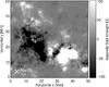 |
Fig. 1 Map of the vertical magnetic field component in the model photosphere at the lower boundary. Marked are the positions of the events shown in Figs. 2 and 4. |
To understand the heating of the corona, it is crucial to study its spatial and temporal evolution. Observations only provide information about consequences but not directly about the heating mechanism and its energy deposition. Therefore we employ a 3D MHD model of the solar atmosphere in order to analyze the spatial and temporal distribution of the heat input. The data used for the present paper is based on a coronal model introduced in Bingert & Peter (2011). The model produces a hot corona above a small active region with self-consistent heating. The heating in the model is due to Ohmic dissipation of free magnetic energy created by the braiding of magnetic field lines. This mechanism of (DC) heating has already been proposed by Parker (1983), where the braiding of field lines is a simplified picture for the energy transport due to the Poynting flux and the subsequent dissipation process. The magnetic fields anchored in the photosphere are shuffled around by photospheric (granular) motions leading to a build-up of currents in the upper atmosphere. The plasma is then heated by dissipation of these currents. Basic parameters derived from the numerical model, such as the energy flux of roughly 100 W m-2 into the corona, match observationally derived values.
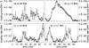 |
Fig. 2 Temporal evolution of the Ohmic heating rate (~j2) at four different locations (single grid-points) in the model corona: a) grid-point with smallest time-averaged heat input, and b) with strongest time-averaged heat input in the coronal volume at T > 105 K; c) location at the top of a bright loop seen in the synthesized coronal emission; and d) at the coronal base at the footpoint of the bright loop. The crosses mark the times of the snapshots. The geometrical heights of these four locations are indicated in Fig. 3. The locations are also indicated in Fig. 1 relative to the photospheric magnetic field. |
The model describes the solar atmosphere above an observed active region depicted in Fig. 1. The domain spans over 50 × 50 Mm2 in the horizontal direction and 30 Mm in the vertical direction. The initial condition for the plasma parameters are given by a hydrostatic plane-parallel atmosphere similar to solar averages. The magnetic field is initially computed using a potential field extrapolation.
The system is then driven by granular motions having the same statistical properties as the photospheric velocities observed on the sun. The evolution of the model atmosphere follows the MHD equations. The lower boundary is prescribed by the granular motions and a fixed plasma pressure. The top boundary is hydrostatic with no heat flux. The magnetic field is extrapolated by matching a potential field at the top. In the horizontal directions the domain is fully periodic.
We ran the model for one solar hour before taking any data to make the result independent of the initial condition. After that we took snapshots with a cadence of 30 s for a bit more than a hour.
For the numerical model we employ the Pencil code (Brandenburg & Dobler 2002). It solves the MHD equations for a compressible, magnetized, viscous fluid. These equations are the conservation of mass, the momentum balance equation, the energy equation, and the induction equation. The Ohmic heating term is given as ημ0j2 with j = ∇ × B/μ0. The time-dependent energy balance in the model includes anisotropic heat conduction (Spitzer 1962), optically thin radiative losses (Cook et al. 1989), together with the viscous and Ohmic heating. No additional arbitrary heating is applied in the model corona, which is sustained almost exclusively through the Ohmic dissipation.
3. Sample events: nanoflares and nanoflare storms
The ohmic heating in the model is transient in time and space. To illustrate this, we show in Fig. 2 the temporal variation in the volumetric heating rate at four grid points of the numerical simulation. These have been selected using the following criteria: (a) the lowest heating rate in the box; (b) the highest heating rate in the coronal volume, i.e., in the region where the temperature exceeds 106 K; (c) at the apex of a loop clearly visible in (synthesized) coronal emission; and (c) at the coronal footpoint of that loop. Obviously these locations span a wide range of (peak) heating rates, covering four orders of magnitude.
In part, this large difference in peak heating is due to the strong drop in the volumetric heating rate with height. In the coronal part, the horizontally averaged volumetric heating rate drops roughly exponentially with a scale height of about 4 Mm, as can be seen from Fig. 3 (the heating per particle shows a peak in the transition region; cf. Bingert & Peter 2011). For example, this drop accounts for a difference in heating rate between locations (a) and (b) in Fig. 2 of about a factor of 100 (cf. dotted lines in Fig. 3). On top of this average drop with height, there is a strong spatial inhomogeneity caused by the structure of the magnetic field and how the magnetic field lines are braided. The magnetic field geometry above 4 Mm (Bingert & Peter 2011) is dominated by a large loop system connecting the main polarities (Fig. 1). At heights above 4 Mm, almost all field lines connect to these polarities. As a result the selected positions do not show any distinguished magnetic configuration.
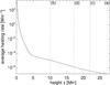 |
Fig. 3 Horizontally and temporally averaged Ohmic heating rate (~j2). The marked postions are at about a) 28 Mm; b) 10 Mm; c) 22 Mm, and d) 17 Mm according to the locations depicted in Fig. 2. |
Most important is that the temporal variability at each position shows a different nature. Referring to Fig. 2, e.g., at location (a) the heating is due to short pulses with a lifetime of a few minutes, whereas at position (b) only one pulse over more than half an hour seems to occur. At positions (c) and (d), the heating is composed of short pulses and of pulses with lifetimes of ten or more minutes. These four profiles represent the complete domain in the sense that the energy is inserted in more or less randomly distributed pulses. Thus it is quite challenging to investigate each of the million gridpoints in the numerical domain. Thus one has to employ a statistical approach. Before we do this in Sect. 4, we investigate one particular location in more detail.
As an illustration we select one spatial location at the very base of the corona and transition region, where the (average) heating rate per particle is highest (see Bingert & Peter 2011). This is shown in Fig. 4. Looking at a spot where the heating rate per particle is at its peak gives some confidence that this is where most of the action is, and thus this example can be considered a representative one.
To estimate the energy deposited in one single burst of heating, the volume covered by this event is needed. The current structures aligned with the magnetic field are typically limited by the spatial resolution of the numerical experiment. Using a high-order scheme to solve the MHD equations, these small structures will have an extent of roughly 4 × 4 × 4 grid points (see also Bingert & Peter 2011, their Fig. 9). This corresponds to a volume of very roughly 2 Mm3 and should be considered as a lower limit.
The temporal evolution in Fig. 4 shows two events in close succession: event (A) consists of several heating pulses occurring shortly one after another so that they merge into one single longer duration event lasting almost 20 min. The second event (B) consists of a single heating pulse with a larger amplitude lasting only a few minutes. (The same is true for the weaker events at times 15 min and 22 min).
When integrating in time and space about 1019 J are deposited during event (A) and a couple of 1017 J are deposited during event (B). These energies coincide roughly with the energy of a typical nanoflare of 1017 J (1024 erg) as originally suggested from theoretical considerations by Parker (1988). Event (B) could then be “classified” as a regular nanoflare. In contrast, event (A) could be related to a nanoflare storm, a phenomenon “with durations of several hundred to several thousand seconds” (Viall & Klimchuk 2011). Originally, these were introduced heuristically to model the light curves of warm loops with the help of 1D models (e.g. Warren et al. 2002), even though this name was coined only later.
Our 3D MHD model with self-consistent Ohmic heating shows that such nanoflare storms are a natural consequence of the braiding of magnetic field lines. Therefore our results support the ad-hoc use of such bursts for the energy release in 1D loop models.
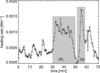 |
Fig. 4 Ohmic heating rate (~j2) at a fixed point in space for more than a solar hour. The data points are marked by crosses. Here a gridpoint at the very base of the corona and transition region (≈3 Mm height) was chosen which is representative of the region where the heating rate per particle is maximal. The large cross in Fig. 2 indicates the horizontal location. The shaded regions (A) and (B) indicate a nanoflare storm and a single nanoflare, see Sect. 3. |
4. Statistical analysis of the heating rate in time
To understand the coronal heating process, it is not sufficient to study single events alone. Instead we have to investigate statistical properties of the heat input. For this we subdivide the computational domain into boxes of equal size V, and the time span of the simulation into time intervals of equal length τ.
As one “event” we define the total energy input through Ohmic heating in one of these boxes with volume V integrated over time τ. For example, if we choose V = (5 × 5 × 5) Mm3 and τ = 5 min, we have 10 × 10 × 6 = 600 boxes in the 50 × 50 × 30 Mm3 domain spread over 12 bins in time for a computational time of 60 min. Consequently we will get 600 × 12 = 7200 individual events for this particular combination of V and τ. We then investigate the statistical properties of these events, in particular their energy distribution. We do this for a variety of combinations of V and τ to show that our results do not depend on a particular choice of V and τ. We choose the subvolumes 0.29 Mm3, 0.97 Mm3, 2.31 Mm3, and 4.51 Mm3, which corresponds to 23, 33, 43, and 53 grid points. The grid spacings are dx = dy = 0.39 Mm and dz = 0.24 Mm. In this approach we use equal-sized noncubic volumes rather than searching for the spatial extent of each individual energy deposition. In Sect. 6 we provide some more details on why this approach is useful and appropriate. A decomposition in real events is rather challenging and perhaps even impossible. The transient heating produces events that not only overlap in time but also overlap in space. Additionally, the energy release shows a general decrease with height, therefore single events will not be easily detectable, except for a few isolated major energy releases. To reduce the investigation to those events, which are clearly seen in the data, would reduce the number of events dramatically, and the statistical analysis would fail.
4.1. Energy distribution of Ohmic dissipation in the whole computational domain (from photosphere to corona)
The procedure described above provides the energies of a large number of events. A common way to analyze this is to investigate the distribution of the energies of these events. If the frequency distribution is normalized by the event energies E, we get a frequency-size distribution. In addition we normalize the frequency-size distribution by the area and time. Here the area is the horizontal extent of the computational domain (50 × 50 Mm2), and the time is the duration of the simulation used in this study (60 min).
Figure 5 depicts the frequency-size distributions f(E) of the Ohmic heating event energies for several combinations of V and τ for the whole computational domain. The event energies range from 1010 J to 1025 J. These are energies several orders of magnitude below and above the energy of a Parker nanoflare that is about 1017 J (1024 erg). The frequency distributions have a roughly constant slope of s ≈ − 1.2 over a wide range, irrespective of the choice of the box size V or the temporal binning τ. Only for high values of V and τ are the number of events too low, and the frequency distribution is not continuous. For instance for the largest binning in space and time we have roughly 8000 boxes, e.g. events, in comparison to the smallest binning with more than 10 million boxes. If the box size increases, small events are missing and the size of the biggest events increases. Therefore the covered energy range of the frequency-size distribution clearly depends on the spatial binning but depends only weakly on the temporal binning.
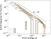 |
Fig. 5 Frequency distribution of Ohmic heating event energies for four different spatial box volumes V and five different temporal bin sizes τ. The temporal binning τ is color−coded and labeled in the figure. The spatial box sizes V are 0.29 Mm3, 0.97 Mm3, 2.31 Mm3, and 4.51 Mm3. The distribution with the smallest box size V is the group of lines starting at the smallest energies (to the left). For the two smallest binnings the number of events is large enough that the frequency size distribution is continuous. For the two larger binnings the distribution is interrupted owing to the low number of events. Overplotted is a power law with a slope of −1.2. The vertical dotted line indicates the typical nanoflare energy as predicted by Parker (1988). See Sect. 4.1. |
As a consistency check, the frequency-size distribution can be used to derive the total energy budget of the system. The total energy flux into the system is given by the integral of the frequency distribution 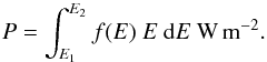 (1)Assuming the frequency distribution to be a power law of the form f(E) = AEs, the energy flux in the range of energies from E1 to E2 is then given by
 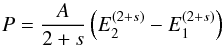 (2)if s ≠ − 2 otherwise P = Aln(E2/E1). If the slope s of the power law is flatter than −2, then the integral is dominated by the upper energy limit. Whereas for slopes steeper than −2 the result is dominated by the lower energy limit.
The slope of the frequency distribution of Ohmic heating events is −1.2 and thus flatter than −2 (cf., Fig. 5). When considering the whole computational domain including the photospheric and chromospheric parts, the majority of heat is therefore deposited in events with high energies.
The energy flux into our modeled box derived from the frequency distribution in Fig. 5 based on Eq. (1) or (2) is on the order of P ≈ 106 W m-2 (= 109 erg s-1 cm-2). This is the flux at the photospheric level, which is the lower boundary of our model atmosphere. This represents the average flux over roughly one hour solar time. It matches nicely with Bingert & Peter (2011), where the energy flux input into the computational domain at a fixed time was found to be in the range between 106 W m-2 and 107 W m-2.
It should be emphasized that these results apply to the whole computational domain, including the photosphere and chromosphere. In Sect. 4.3 we discuss the energy distribution and budget for the coronal part of the domain alone.
4.2. Power-law test for energy distribution
Even if the slope of the distribution functions of the Ohmic heating events looks fairly constant over several orders of magnitude, we briefly discuss how to test the validity of the assumption that this is indeed a power law. It can be problematic to use linear regression in a log-log plot to retrieve the slope of a power law. Therefore we follow Virkar & Clauset (2012) and use a maximum-likelihood estimation (MLE) to obtain the slope of a possible power law. As discussed in Virkar & Clauset (2012), the result is sensitive to the selection of the lower energy cutoff. In Table 1 we list the estimated slopes following from the MLE technique for various combinations of the spatial box sizes V and time bins τ for the events. We neglect 5% of the lowest energies from the analysis.
Having derived a slope is not yet a proof for a power-law. Again we follow Virkar & Clauset (2012) and use the Kolmogorov-Smirnov test (Press et al. 1992) to check whether the distribution functions match the power laws. The slopes retrieved by the MLE give a confidence level above 0.9 for the two distribution functions with smallest spatial binnings (cf., Fig. 5). The highest confidence levels we find are for a slope of 1.20. All slopes discussed here are around 1.2, and the confidence levels are high enough to argue that the distributions of Ohmic heating events are consistent with power laws.
4.3. Heating statistics for the coronal part alone
We now focus on the coronal part. We define the coronal part either through a threshold in temperature or as the volume above a certain height. Both definitions (when properly chosen) give similar results. This will give us information about the distribution of the heat input into the model corona. Therefore, we repeat the analysis from Sect. 4.1 in the subvolume of the computational domain representing the corona and the transition region.
To define the coronal volume, in the first case we choose a temperature threshold of log T/[K] = 3.9 to include everything above the chromosphere. In the second case we define the coronal volume as being at heights above 4 Mm. This corresponds to the height where the horizontally averaged temperature exceeds log T/ [K] = 3.9 in our model. It is also the height where the scale height of the horizontally averaged volumetric heating rate increases and becomes constant for the coronal part (see Fig. 3 and Bingert & Peter 2011). The model atmosphere is very dynamic so that the isosurface for a constant temperature is highly corrugated. The height variation of the isothermal surface of log T/ [K] = 3.9 is several Mm. This is larger than to the chromospheric scale height, but much smaller than the coronal scale height. In particular, this is much smaller than the vertical extent of the coronal part of our computational domain. This is the basic reason, why the results for these two methods will be essentially the same.
When now considering the coronal volume alone (using the above two definitions), the event energies show a distribution that is composed of two power laws, with a knee at about 1017 J, and a slope of − 1.2 below and − 2.5 above the knee (see Fig. 6). The slope at small-event energies is comparable to Fig. 5 as found for the whole computational domain. For energies below 1014 J the distribution shows the typical cut off due to limited resolution and statistics. Here and in the following we only show the results for one particular choice of the spatial box size V and temporal binning τ to determine the distribution of event energies (V = 0.29 Mm3, τ = 5 min). This is only to not clutter the plots, the results are independent of the particular choice of V and τ (cf. Sect. 6). The distribution in Fig. 6 represents a subsample of the complete computational domain so that the range of the covered event energies is smaller than for the analysis of the entire domain shown in Fig. 5.
The result that the slope of the power law is flatter than − 2 below 1017 J and steeper than − 2 above has a very pointed consequence. Below the knee most of the energy is deposited at higher energies, i.e., close to the knee. Above the knee most of the deposition is at low energies, i.e., again close to the knee. Therefore most of the energy will be deposited close to the knee at 1017 J, which coincides with the originally proposed energy for nanoflares.
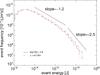 |
Fig. 6 Distribution of Ohmic heating event energies in the coronal volume alone. The results are shown for two definitions of the coronal volume: a) log T[K] > 3.9 and b) heights z > 4 [Mm]. Results are shown only for V = 0.29 Mm3, τ = 5 min). Overplotted are lines indicating power laws with slopes of −1.2 and −2.5, respectively. See Sect. 4.3. |
A more quantitive way to locate the main contribution to the heat input in terms of event energies is to evaluate the energy deposited in different energy ranges. For this, we integrate the frequency distribution in Fig. 6 piecewise with a fixed interval in Δlog E [J] = 0.2 around the energy E0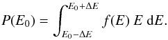 (3)This gives the total energy flux into the corona that is deposited in a range of event energies centered on E0. Figure 7 shows the distribution of there energy fluxes P(E0) as a function of the event energy E0. The maximum flux is found at an energy of roughly 1017 J (1024 erg) just as suspected above. The integration is performed using an interpolation of initial distribution. But using the original resolution in energy does not alter the results, and only the width of the bins would be broader. The error for the peak flux is estimated by the half bin width of initial data, e.g, 0.16 or a factor of roughly 1.4
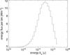 |
Fig. 7 Energy fluxes into the corona deposited at different energies E0 of the heating events. Derived from the distribution in Fig. 6. The distribution is first interpolated to allow for an integration interval of 0.2 dex in logarithmic values. See Sect. 4.3. |
As a sanity check, we can use the result shown in Fig. 7 to compute the total energy input to the model corona by integrating over the whole range of energies. We find this to be 100 W m-2, which is consistent with the results given by Bingert & Peter (2011) and consistent with estimations of the coronal heating requirements based on observations (Withbroe & Noyes 1977).
This result of the distribution of energy fluxes in Fig. 7 shows that the upper atmosphere in our model is mainly heated by events with an energy of a few times 1017 J, which roughly matches the typical nanoflare energy. In addition to the qualitative discussion of the position of the knee in Fig. 6, this quantitative result also provides information on the range of energies responsible for the energy input. From Fig. 7 it is clear that energies from 1016 to 1018 J (1023 to 1025 erg) contribute significantly.
From this we can conclude that in our 3D MHD model there is a preferred energy for the deposition through Ohmic heating. This value is the same order of magnitude as the nanoflare energies derived by Parker (1988) on theoretical grounds, despite all the limitations in terms of spatial resolution and magnetic Reynolds number in our numerical experiments. This is reassuring, because our 3D MHD model basically describes the flux-braiding process as proposed by Parker (1988).
5. Consequences for observable quantities
The frequency-size distributions derived in the previous section are based on the energy deposition due to Ohmic dissipation. However, these events with energies close to the values of nanoflare energies are not directly observable on the Sun. For an observational study of the region where the plasma is heated, the only source of information we have is the emission in exteme UV and X-rays. And this provides only partial information on the energy budget, because heat conduction, particle acceleration, and maybe other processes will also redistribute the energy, which will then be, e.g., radiated in other places.
To study how the distribution of energies changes if one investigates the brightenings related to the heating events, we synthesize the expected optically thin coronal and transition region emission from the MHD model. Here we follow the procedure outlined by Peter et al. (2004, 2006). To derive reliable estimates of the coronal emission, the MHD model has to treat the energy equation appropriately; in particular it is essential to include the heat conduction to self-consistently set the proper coronal pressure (and thus density). Using the CHIANTI atomic data base (Dere et al. 1997; Landi et al. 2006), we calculate the emission at each grid point for a number of emission lines based on the temperature and density at the respective gridpoint in the model. The result is the volumetric energy loss per second through optically thin radiation in a given spectral line.
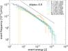 |
Fig. 8 Event frequency distributions of synthesized emission lines. The name of the lines are given in the legend along with the wavelength [Å] and the line formation temperature in log T/ [K]. |
We repeat the analysis of the preceding section and treat the emission in each of the lines in the same way as the energy input in Sects. 4.1 and 4.3. Figure 8 shows the resulting distribution functions for the radiative energy loss events. The energy range is shifted to much lower energies than in Figs. 5 and 6. This is mainly because each line only represents one single emission line, and each emission line contributes only a small fraction of the total energy loss. Nonetheless, the distribution functions show similar power laws for all emission lines with line formation temperatures ranging from 30 000 K up to 106 K. Owing to the different formation temperatures, the lines originate from different densities, so that the frequency distributions have different cut-offs at the high-energy end.
Most importantly, the power law shows a slope of about − 0.8. This slope is slightly flatter at low energies and a bit steeper for high energies, but is flatter than the slope of − 1.2 found for the energy input. The reduction of the slope reflects the nonlinear connection from heat input to the final (optically thin) radiative output. There are basically two ways of looking at this phenomenon: (1) a heuristic explanation based on the energy redistribution and (2) a more formal argument using scaling laws.
At coronal temperatures heat conduction dominates radiative losses (e.g. Priest 1982); the higher the temperature, the more heat conduction dominates (below 107 K). On average, the heat input (per volume and time) is smaller at higher temperatures at larger heights (Fig. 3), where the energy input is lower. Thus heat conduction is the major loss process at the low-energy end of the distribution of event energies. Consequently, there is less radiation at the low-energy end, and the distribution of the radiative losses will be flatter, in our case the slope is only − 0.8 instead of − 1.2.
The same mechanism also explains why the knee in the energy input (Fig. 6; Sect. 4.3) is not clearly visible in the distribution of the radiative losses (Fig. 8). The energy deposited around the nanoflare energies coinciding with the location of the knee is mainly transported down towards the chromosphere, i.e. towards the high-energy end of the distribution, and is then radiated at lower temperatures in the transition region. In turn, this enhances the distribution at the high-energy end of the distribution of the radiative output.
To get a quantitative estimate of the flattening of the power-law slope from the energy input (− 1.2) to the radiative output (− 0.8), we investigate the scaling laws as already described by Rosner et al. (1978). The scaling laws relate the volumetric heat input EH (assumed to be constant) and the loop length L to the peak temperature T and pressure p of a hydrostatic loop (Eqs. (4.3) and (4.4) of Rosner et al. 1978). One can easily combine these to relate the density n at the apex to the heat input and loop length,  . Because the dependence on L is weak, we discard this in the following. The energy loss ε due to optically thin radiation (per volume and time) is proportional to the density squared, ε ∝ n2, and with the above scaling law we find ε ∝ (EH)8/7. Therefore the slope of the power law should change from − 1.2 to − 1.2 × 7/8 = −1.05. This change does go in the right direction, but does not quite explain the result of − 0.8 we find in Fig. 8. This is not very surprising, because the Rosner et al. (1978) scaling laws apply only to hydrostatic loops with a constant heating rate, while our 3D MHD model is time-dependent with a nonconstant heating rate.
In conclusion, the energy events for the radiative losses are still distributed as a power law, but the slope is flatter than the power law for the actual energy input. This is important for observational studies investigating the energy input by analyzing the energy loss through brightenings seen in EUV and X-rays.
6. Self-organized criticality and fractal dimension
In Sect. 4 we derived the frequency-size distributions for Ohmic heating events. These distributions follow a power law over several orders of magnitude (Fig. 5). This power law does not change if the binning of the data cube is changed, either spatially or temporally. This behavior is typical of a power-law frequency-size distribution, so it indicates that our modeled energy input also follows a power law. Systems that are characterized by a power law are called self-organized critical systems (Bak et al. 1987). Self-organized criticality can also be applied to other systems such as 1/f noise, and it shows the scale invariance of the system on a macroscopic level. This scale invariance manifests itself by the fact that the slopes of the power laws are independent of the spatial scale range under consideration, i.e. of the spatial binning. Therefore the approach of using a constant binning for the analysis in Sects. 4.1 and 4.3 does not affect the results. The constant binning refers to equally sized volumes. Likewise the noncubic boxes do not alter the result since we can use arbitrary volumes in a scale-independent system.
We find in our analysis that the frequency size distribution of the event energies can be represented by a single slope alone. This is consistent with other model approaches, e.g, Dimitropoulou et al. (2011) and Georgoulis et al. (2001), and with observations (Aschwanden & Freeland 2012). In earlier studies Georgoulis & Vlahos (1996) and Georgoulis & Vlahos (1998) used cellular automata models and find a double power law behavior for the event size. That our distribution functions follow a single power law can be accounted for by the short time period of one hour and by the small field of few of our model active region.
Following Aschwanden (2010) the slope of the power law of the distribution functions point to the propagation properties of the instability leading to the dissipative events. The fractal dimension D is thereby correlated to the slope s by D = 3/s (Aschwanden 2010; Aschwanden & Freeland 2012). Since we measure a slope of 1.2, the fractal dimension of the system would be 2.5 for the Ohmic dissipation events. This means that the fractal dimension is not bound to the 2D surface of separatrix layers, and that the propagation of the instability cannot spread freely in all three dimensions.
Formally, using the slope of − 1 of the power law for the radiative losses (Fig. 8), we find a fractal dimension of 3. However, because the emission is just a secondary quantity following from the heat input and strongly affected by the heat conduction, the diagnostic value of this result is limited, though.
7. Conclusions
In Sect. 3 we discussed the transient nature of the heating based on time series of the Ohmic heating at specific locations. There the temporal evolution of the heating rate shows a stochastic nature, as well as a qualitative difference at different places. We saw long bursts (10 min and longer), which may consist of several short pulses. At other locations we saw only short pulses (1 min and less). These events could correspond to the nanoflare storms and nanoflares often assumed in 1D loop models (Viall & Klimchuk 2011). We used these time series only for a qualitative description and for a rough estimate of the magnitude of heating events. We saw that these events deposit energies on the order of 1017 J, which agrees with the nanoflare energy estimated by Parker (1988).
We also presented a more sophisticated approach using statistical methods to analyze these events in the complete domain. The statistical analysis of the coronal heating reveals a power law for the heating event energies. Even though the driver, i.e. the granular motion, does not work on all scales, the slope of the power law is constant over several orders of magnitude and flatter than −2. We find that in the transition region and corona the dominant energy for the heating events is the nanoflare energy, i.e. 1017 J. Since the higher energy events occur on average at lower heights, the heating is footpoint-dominated. The event energies we find in our model are below the detection limit of current instrumentation and support the scenario of nanoflare heating as proposed by Parker (1988).
In our model the energy provided by the field-line braiding is converted into heating through Ohmic dissipation and not into particle acceleration. This implies that nonlocal effects are not incorporated. This is justified by the electron mean-free-path being smaller than the grid spacing of the model. The energy is redistributed by advection and conduction or radiated by optically thin emission. From our model atmosphere we synthesized observable extreme UV emission lines. The statistical analysis of these lines shows again a power-law behavior. The slope of this power law is around 1 and smaller than the slope of the heating process. Even though the power law is maintained over several orders of magnitude, in contrast to the heating process, the radiative losses are not in a self-organized critical state. This is because the radiative losses are coupled to the heating in a nonlinearly.
In this study we showed that a 3D MHD model of the active region solar corona has a preferred energy for depositing of heat through Ohmic dissipation following field-line braiding. The preferred energy of about 1017 J (1024 erg) corresponds well to the value derived by Parker (1988) and thus is yet another piece of evidence that, despite all their shortcomings, the 3D MHD
models for the flux-braiding mechanism provide a good description of the heating of the solar corona in active regions.
References
- Akabane, K. 1956, PASJ, 8, 173 [NASA ADS] [Google Scholar]
- Aschwanden, M. J. 2010 [arXiv:1008.0873] [Google Scholar]
- Aschwanden, M. J., & Freeland, S. L. 2012, ApJ, 754, 112 [NASA ADS] [CrossRef] [Google Scholar]
- Bak, P., Tang, C., & Wiesenfeld, K. 1987, Phys. Rev. Lett., 59, 381 [NASA ADS] [CrossRef] [PubMed] [Google Scholar]
- Bingert, S., & Peter, H. 2011, A&A, 530, A112 [NASA ADS] [CrossRef] [EDP Sciences] [Google Scholar]
- Brandenburg, A., & Dobler, W. 2002, Comput. Phys. Commun., 147, 471 [NASA ADS] [CrossRef] [Google Scholar]
- Charbonneau, P., McIntosh, S. W., Liu, H.-L., & Bogdan, T. J. 2001, Sol. Phys., 203, 321 [NASA ADS] [CrossRef] [Google Scholar]
- Christe, S., Hannah, I. G., Krucker, S., McTiernan, J., & Lin, R. P. 2008, ApJ, 677, 1385 [NASA ADS] [CrossRef] [Google Scholar]
- Cook, J. W., Cheng, C., Jacobs, V. L., & Antiochos, S. K. 1989, ApJ, 338, 1176 [NASA ADS] [CrossRef] [Google Scholar]
- Crosby, N. B., Aschwanden, M. J., & Dennis, B. R. 1993, Sol. Phys., 143, 275 [NASA ADS] [CrossRef] [Google Scholar]
- Crosby, N., Vilmer, N., Lund, N., & Sunyaev, R. 1998, A&A, 334, 299 [NASA ADS] [Google Scholar]
- Dere, K. P., Landi, E., Mason, H. E., Monsignori Fossi, B. C., & Young, P. R. 1997, A&AS, 125, 149 [NASA ADS] [CrossRef] [EDP Sciences] [Google Scholar]
- Dimitropoulou, M., Isliker, H., Vlahos, L., & Georgoulis, M. K. 2011, A&A, 529, A101 [NASA ADS] [CrossRef] [EDP Sciences] [Google Scholar]
- Georgoulis, M. K., & Vlahos, L. 1996, ApJ, 469, L135 [NASA ADS] [CrossRef] [Google Scholar]
- Georgoulis, M. K., & Vlahos, L. 1998, A&A, 336, 721 [NASA ADS] [Google Scholar]
- Georgoulis, M. K., Vilmer, N., & Crosby, N. B. 2001, A&A, 367, 326 [NASA ADS] [CrossRef] [EDP Sciences] [Google Scholar]
- Gudiksen, B., & Nordlund, Å. 2002, ApJ, 572, L113 [Google Scholar]
- Gudiksen, B., & Nordlund, Å. 2005a, ApJ, 618, 1020 [NASA ADS] [CrossRef] [Google Scholar]
- Gudiksen, B., & Nordlund, Å. 2005b, ApJ, 618, 1031 [NASA ADS] [CrossRef] [Google Scholar]
- Hannah, I. G., Hudson, H. S., Battaglia, M., et al. 2011, Space Sci. Rev., 159, 263 [NASA ADS] [CrossRef] [Google Scholar]
- Hansteen, V. H., Hara, H., De Pontieu, B., & Carlsson, M. 2010, ApJ, 718, 1070 [Google Scholar]
- Landi, E., Del Zanna, G., Young, P. R., et al. 2006, ApJS, 162, 261 [NASA ADS] [CrossRef] [Google Scholar]
- Lu, E. T. 1995, ApJ, 446, L109 [NASA ADS] [CrossRef] [Google Scholar]
- Lu, E. T., & Hamilton, R. J. 1991, ApJ, 380, L89 [NASA ADS] [CrossRef] [Google Scholar]
- Parker, E. N. 1983, ApJ, 264, 642 [NASA ADS] [CrossRef] [Google Scholar]
- Parker, E. N. 1988, ApJ, 330, 474 [Google Scholar]
- Peter, H. 2007, Adv. Space Res. 39, 1814 [Google Scholar]
- Peter, H., & Bingert, S. 2012, A&A, 548, A1 [NASA ADS] [CrossRef] [EDP Sciences] [Google Scholar]
- Peter, H., & Judge, P. G. 1999, ApJ, 522, 1148 [NASA ADS] [CrossRef] [Google Scholar]
- Peter, H., Gudiksen, B., & Nordlund, Å. 2004, ApJ, 617, L85 [NASA ADS] [CrossRef] [Google Scholar]
- Peter, H., Gudiksen, B., & Nordlund, Å. 2006, ApJ, 638, 1086 [NASA ADS] [CrossRef] [MathSciNet] [Google Scholar]
- Press, W. H., Teukolsky, S. A., Vetterling, W. T., & Flannery, B. P. 1992, Numerical recipes in C. The art of scientific computing [Google Scholar]
- Priest, E. R. 1982, Solar Magnetohydrodynamics (Dordrecht: D. Reidel) [Google Scholar]
- Rosner, R., & Vaiana, G. S. 1978, AJ, 222, 1104 [NASA ADS] [CrossRef] [Google Scholar]
- Rosner, R., Tucker, W. H., & Vaiana, G. S. 1978, ApJ, 220, 643 [NASA ADS] [CrossRef] [Google Scholar]
- Spitzer, L. 1962, Physics of fully ionized gases, 2nd edn. (New York: Interscience) [Google Scholar]
- Viall, N. M., & Klimchuk, J. A. 2011, ApJ, 738, 24 [Google Scholar]
- Virkar, Y., & Clauset, A. 2012, e-prints [arXiv:1208.3524] [Google Scholar]
- Warren, H. P., Winebarger, A. R., & Hamilton, P. S. 2002, ApJ, 579, L41 [NASA ADS] [CrossRef] [Google Scholar]
- Withbroe, G. L., & Noyes, R. W. 1977, ARA&A, 15, 363 [NASA ADS] [CrossRef] [Google Scholar]
- Zacharias, P., Bingert, S., & Peter, H. 2011, A&A, 531, A97 [NASA ADS] [CrossRef] [EDP Sciences] [Google Scholar]
All Tables
All Figures
|
Fig. 1 Map of the vertical magnetic field component in the model photosphere at the lower boundary. Marked are the positions of the events shown in Figs. 2 and 4. |
| In the text | |
|
Fig. 2 Temporal evolution of the Ohmic heating rate (~j2) at four different locations (single grid-points) in the model corona: a) grid-point with smallest time-averaged heat input, and b) with strongest time-averaged heat input in the coronal volume at T > 105 K; c) location at the top of a bright loop seen in the synthesized coronal emission; and d) at the coronal base at the footpoint of the bright loop. The crosses mark the times of the snapshots. The geometrical heights of these four locations are indicated in Fig. 3. The locations are also indicated in Fig. 1 relative to the photospheric magnetic field. |
| In the text | |
|
Fig. 3 Horizontally and temporally averaged Ohmic heating rate (~j2). The marked postions are at about a) 28 Mm; b) 10 Mm; c) 22 Mm, and d) 17 Mm according to the locations depicted in Fig. 2. |
| In the text | |
|
Fig. 4 Ohmic heating rate (~j2) at a fixed point in space for more than a solar hour. The data points are marked by crosses. Here a gridpoint at the very base of the corona and transition region (≈3 Mm height) was chosen which is representative of the region where the heating rate per particle is maximal. The large cross in Fig. 2 indicates the horizontal location. The shaded regions (A) and (B) indicate a nanoflare storm and a single nanoflare, see Sect. 3. |
| In the text | |
|
Fig. 5 Frequency distribution of Ohmic heating event energies for four different spatial box volumes V and five different temporal bin sizes τ. The temporal binning τ is color−coded and labeled in the figure. The spatial box sizes V are 0.29 Mm3, 0.97 Mm3, 2.31 Mm3, and 4.51 Mm3. The distribution with the smallest box size V is the group of lines starting at the smallest energies (to the left). For the two smallest binnings the number of events is large enough that the frequency size distribution is continuous. For the two larger binnings the distribution is interrupted owing to the low number of events. Overplotted is a power law with a slope of −1.2. The vertical dotted line indicates the typical nanoflare energy as predicted by Parker (1988). See Sect. 4.1. |
| In the text | |
|
Fig. 6 Distribution of Ohmic heating event energies in the coronal volume alone. The results are shown for two definitions of the coronal volume: a) log T[K] > 3.9 and b) heights z > 4 [Mm]. Results are shown only for V = 0.29 Mm3, τ = 5 min). Overplotted are lines indicating power laws with slopes of −1.2 and −2.5, respectively. See Sect. 4.3. |
| In the text | |
|
Fig. 7 Energy fluxes into the corona deposited at different energies E0 of the heating events. Derived from the distribution in Fig. 6. The distribution is first interpolated to allow for an integration interval of 0.2 dex in logarithmic values. See Sect. 4.3. |
| In the text | |
|
Fig. 8 Event frequency distributions of synthesized emission lines. The name of the lines are given in the legend along with the wavelength [Å] and the line formation temperature in log T/ [K]. |
| In the text | |
Current usage metrics show cumulative count of Article Views (full-text article views including HTML views, PDF and ePub downloads, according to the available data) and Abstracts Views on Vision4Press platform.
Data correspond to usage on the plateform after 2015. The current usage metrics is available 48-96 hours after online publication and is updated daily on week days.
Initial download of the metrics may take a while.