© ESO, 2013

1. Introduction

The X-ray-to-UV ratio of active galactic nuclei (AGN) gives direct information on an important region of the spectral energy distribution (SED), relating the radiative processes that operate in the accretion disk and in the corona, connecting their emissions across the unobservable band of the extreme UV. It characterises the shape of the SED, and affects, through the ionisation equilibrium, properties of the UV spectral lines, such as the equivalent width and the blue-shift of the CIV λ1549 emission line (Richards et al. 2011).

The X-ray/UV ratio is often expressed through the inter-band spectral index ${\mathit{\alpha }}_{\mathrm{ox}}\mathrm{\equiv }\frac{\log \hspace{0.17em}\mathrm{(}{\mathit{L}}_{\mathit{X}}\mathit{/}{\mathit{L}}_{\mathrm{UV}}\mathrm{)}}{\log \hspace{0.17em}\mathrm{(}{\mathit{\nu }}_{\mathit{X}}\mathit{/}{\mathit{\nu }}_{\mathrm{UV}}\mathrm{)}}\mathrm{=}\mathrm{0.384}\log \left(\frac{{\mathit{L}}_{\mathit{X}}}{{\mathit{L}}_{\mathrm{UV}}}\right)$(1)between the conventional frequencies ν_X ≡ ν_2keV and ν_UV ≡ ν_2500 Å.

α_ox is found to be strongly anti-correlated with the ultraviolet specific luminosity L_UV, showing that more luminous objects are, on average, relatively weaker in X-rays: ${\mathit{\alpha }}_{\mathrm{ox}}\mathrm{=}\mathit{a}\log {\mathit{L}}_{\mathrm{UV}}\mathrm{+}\mathrm{const} \mathrm{(}\mathit{a}\mathit{<}\mathrm{0}\mathrm{)}\hspace{0.17em}\mathit{.}$(2)This relation has been studied by many authors, who found slopes approximately in the interval −0.2 ≲ a ≲ −0.1 (e.g., Strateva et al. 2005; Steffen et al. 2006; Just et al. 2007; Gibson et al. 2008; Grupe et al. 2010; Vagnetti et al. 2010), depending on the selection of the sample, and especially on its range of luminosities and/or redshifts. For instance, while Just et al. (2007) derived a =  −0.14 within a wide area of the L − z plane, 27.5 < log L_UV < 33, 0 < z < 6, a flatter slope was found by Grupe et al. (2010), a =  −0.114, for a low-luminosity and low-redshift sample, 26 < log L_UV < 31, z < 0.35, and a steeper slope, a =  −0.217, was obtained by Gibson et al. (2008) for higher redshifts and luminosities, 30.2 < log L_UV < 31.8, 1.7 < z < 2.7. A similar trend was found dividing a wider sample into two subsamples with lower and higher luminosity or redshift, see e.g. Steffen et al. (2006); Vagnetti et al. (2010). Thus, a precise estimate of the slope cannot be given in general terms, as the α_ox − L_UV relation itself might be non-linear.

Moreover, Gibson et al. (2008) noticed the large scatter of the data around the average relation, suggesting that a large part of it can be caused by variability, combined with non-simultaneity of the X-ray and optical observations. In a previous paper (Vagnetti et al. 2010, Paper I), we have analysed a sample with simultaneous measurements extracted from the XMM-Newton Serendipitous Source Catalogue (Watson et al. 2009), concluding that artificial α_ox variability due to non-simultaneity is not the main cause of dispersion, while intrinsic α_ox variability of individual sources (or intra-source dispersion) and intrinsic differences in the time-average values of α_ox from source to source (or inter-source dispersion) are the most important contributions.

In Paper I, we then analysed the α_ox variability computing the ensemble structure function, and pointed out the need of more AGN samples with simultaneous measurements to make progress in this topic. Appropriate data can be obtained by space observatories that have both X-ray and optical/UV telescopes on board, such as XMM-Newton and Swift.

In this paper, we present the analysis of a sample of low-redshift AGNs observed by Swift that were previously studied by Grupe et al. (2010), whose paper and sample will hereafter be referred to as G10.

This paper is organised as follows. Section 2 describes the data extracted from G10 and from the Swift archive. Section 3 analyses the α_ox − L_UV anti-correlation and its dispersion. In Sect. 4, we present the ensemble structure function of the intrinsic X/UV variability. Section 5 discusses and summarises the results.

Throughout the paper, we adopt the cosmology H₀ = 70 km s^-1 Mpc^-1, Ω_m = 0.3, and Ω_Λ = 0.7.

2. Data

The G10 sample consists of 92 AGNs extracted from the bright soft X-ray selected sample of Grupe et al. (2001), which was observed with Swift between 2005 and 2010. The sample by Grupe et al. (2001) contains all 110 Seyfert galaxies from the sample of 397 sources by Thomas et al. (1998), which was extracted from the ROSAT All Sky Survey (Voges et al. 1999) to include sources selected to be X-ray bright (count rate >0.5 counts/s), X-ray soft (hardness ratio¹ HR < 0.0), and at high Galactic latitude (|b|  > 20°).

The G10 sample includes simultaneous X-ray and optical/UV measurements for most of the sources, and in many cases multi-epoch observations are available, with a total of 299 observations for the 92 sources. However, in a few cases the data are not usable for our purposes, because of lack of X-ray or optical/UV measurements. We therefore adopted a preliminary subsample of 90 sources, with 74 multi-epoch sources and 16 single-epoch sources, for a total of 241 observations. In the following analysis (Sect. 2.1), we removed a few observations whose determination of the AGN luminosity is unreliable, because of strong dominance of the host galaxy, or because of insufficient spectral coverage of the optical/UV data. We define the resulting set of 216 observations as sample A, including 86 sources (68 multi-epoch and 18 single-epoch). In Sect. 3, we introduce another subsample that does not contain known radio-loud sources, which we call sample B. The data are taken from the tables of the G10 paper, which are available electronically, and were checked through the Swift archive at Heasarc².

Compared to the sample of Paper I, the sample studied in the present paper lies in a region of the luminosity-redshift plane at lower redshifts (z < 0.35) and luminosities (26 < log L_UV < 31), see Fig. 1. The relevant properties of the sources of samples A and B at each epoch are reported in Table 1, where Col. 1 corresponds to the source serial number according to G10; Col. 2 to the source name; Col. 3 to the observation epoch serial number; Col. 4 to the epoch in modified Julian days (MJD); Col. 5 to the redshift; Col. 6 to the soft X-ray spectral index, according to Table 4 of G10; Col. 7 to the logarithm of the specific luminosity at 2 keV in erg s^-1 Hz^-1; Col. 8 to the logarithm of the specific AGN luminosity at 2500 Å in erg s^-1 Hz^-1; Col. 9 to the logarithm of the specific host galaxy luminosity at 2500 Å in erg s^-1 Hz^-1 (substituted by a hyphen when the galaxy contribution is negligible); Col. 10 to the optical/X-ray spectral index; and Col. 11 to the radio-loudness flag f_RL = 1 (radio-loud), f_RL = 0 (radio-quiet), f_RL =  −1 (unclassified).

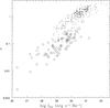Fig. 1 Distribution of the sources in the LUV-z plane. Open circles: Swift sample; dots: XMM-Newton sample.

2.1. UV luminosities

The UltraViolet/Optical Telescope (UVOT) onboard Swift has six photometric filters, whose central wavelengths are λ(V) = 5468 Å, λ(B) = 4392 Å, λ(U) = 3465 Å, λ(UVW1) = 2600 Å, λ(UVM2) = 2246 Å, and λ(UVW2) = 1928 Å (Roming et al. 2005, 2009). Magnitudes in one or more of these bands are available for each source and epoch of our sample from Table 3 of G10. We first transformed magnitudes to fluxes according to the formulae given by Poole et al. (2008), using the count rate-to-flux conversion factors of their table 10 (GRB models, also appropriate for AGNs). To estimate UV luminosities at 2500 Å, similarly to the procedure used in Paper I, we computed, from each of the available fluxes, the corresponding luminosities as ${\mathit{L}}_{\mathit{\nu }}\mathrm{\left(}{\mathit{\nu }}_{\mathrm{rest}}\mathrm{\right)}\mathrm{=}{\mathit{F}}_{\mathit{\nu }}\mathrm{\left(}{\mathit{\nu }}_{\mathrm{obs}}\mathrm{\right)}\hspace{0.17em}\mathrm{4}\mathit{\pi }{\mathit{D}}_{\mathrm{L}}^{\mathrm{2}}\mathit{/}\mathrm{(}\mathrm{1}\mathrm{+}\mathit{z}\mathrm{)}$, and derived the rest-frame SEDs, which are shown in Fig. 2.

Then, we took into account the contribution of the host galaxy starlight, which can be significant for AGNs of low luminosity such as those considered here. Following a procedure similar to that adopted by Lusso et al. (2010), we modelled the optical spectrum by a combination of AGN and galaxy components as ${\mathit{L}}_{\mathit{\nu }}\mathrm{=}\mathit{A}\mathrm{\left[}{\mathit{f}}_{\mathrm{A}}{\mathit{F}}_{\mathrm{R}}\mathrm{\right(}\mathit{\nu }\mathrm{)}\mathrm{+}{\mathit{f}}_{\mathrm{G}}\mathrm{(}\mathit{\nu }\mathit{/}{\mathit{\nu }}_{\mathrm{\ast }}{\mathrm{)}}^{-3}\mathrm{]}\mathit{,}$(3)where F_R(ν) is the mean SED computed by Richards et al. (2006) for type 1 quasars from the Sloan Digital Sky Survey (SDSS), A is a normalisation factor, and the coefficients f_G and f_A represent the galaxy and AGN fractional contributions at the frequency ν_∗, corresponding to 2500 Å (log ν_∗ = 15.08). The average spectral index α_opt of Eq. (3) is a monotonic function of the ratio f_G/f_A, which is thus determined by comparison with the slope of each observed SED. A clear sign of this dependence is apparent in Fig. 2, where less luminous sources have progressively steeper spectra.

The normalisation factor A is then fitted to the data by general linear least-squares (Press et al. 1992) as $\mathit{A}\mathrm{=}\frac{{\sum }_{\mathit{i}\mathrm{=}\mathrm{1}}^{\mathit{N}}{\mathit{y}}_{\mathit{i}}\mathit{X}\mathrm{\left(}{\mathit{\nu }}_{\mathit{i}}\mathrm{\right)}\mathit{/}{\mathit{\sigma }}_{\mathit{i}}^{\mathrm{2}}}{{\sum }_{\mathit{i}\mathrm{=}\mathrm{1}}^{\mathit{N}}\mathrm{\left[}\mathit{X}\mathrm{\right(}{\mathit{\nu }}_{\mathit{i}}\mathrm{)}{\mathrm{]}}^{\mathrm{2}}\mathit{/}{\mathit{\sigma }}_{\mathit{i}}^{\mathrm{2}}}\mathit{,}$(4)where X(ν_i) = log L_ν(ν_i) is given by the model function of Eq. (3) computed in correspondence to the available UVOT rest-frame frequencies ν_i, y_i = log L_i is given by the corresponding measured specific luminosities, and σ_i are their errors. This procedure determines the luminosities of the two components at 2500 Å, L_AGN and L_G, for each source and epoch. In most cases, we can compare the different determinations of L_G for the same source at more epochs, finding low dispersions (usually ≲0.15 in log L_G). 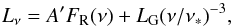We then fixed L_G to its average value for each source and repeated the fit to the data, modifying the fitting function as ${\mathit{L}}_{\mathit{\nu }}\mathrm{=}{\mathit{A}}^{\mathrm{\prime }}{\mathit{F}}_{\mathrm{R}}\mathrm{\left(}\mathit{\nu }\mathrm{\right)}\mathrm{+}{\mathit{L}}_{\mathrm{G}}\mathrm{(}\mathit{\nu }\mathit{/}{\mathit{\nu }}_{\mathrm{\ast }}{\mathrm{)}}^{-3}\mathit{,}$(5)where the factor A′ is now given by ${\mathit{A}}^{\mathrm{\prime }}\mathrm{=}\frac{{\sum }_{\mathit{i}\mathrm{=}\mathrm{1}}^{\mathit{N}}{\mathit{y}}_{\mathit{i}}^{\mathrm{\prime }}{\mathit{X}}^{\mathrm{\prime }}\mathrm{\left(}{\mathit{\nu }}_{\mathit{i}}\mathrm{\right)}\mathit{/}{\mathit{\sigma }}_{\mathit{i}}^{\mathrm{2}}}{{\sum }_{\mathit{i}\mathrm{=}\mathrm{1}}^{\mathit{N}}\mathrm{\left[}{\mathit{X}}^{\mathrm{\prime }}\mathrm{\right(}{\mathit{\nu }}_{\mathit{i}}\mathrm{)}{\mathrm{]}}^{\mathrm{2}}\mathit{/}{\mathit{\sigma }}_{\mathit{i}}^{\mathrm{2}}}\mathit{,}$(6)with X′(ν_i) = log F_R(ν_i), and ${\mathit{y}}_{\mathit{i}}^{\mathrm{\prime }}\mathrm{=}\log \mathrm{[}{\mathit{L}}_{\mathit{i}}\mathrm{-}{\mathit{L}}_{\mathrm{G}}\mathrm{(}{\mathit{\nu }}_{\mathit{i}}\mathit{/}{\mathit{\nu }}_{\mathrm{\ast }}{\mathrm{)}}^{-3}\mathrm{]}$. The AGN luminosity at 2500 Å is then given by L_AGN = A′F_R(ν_∗). In the following, we refer to it simply as L_UV, maintaining the name L_G for the galactic contribution.

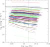Fig. 2 Spectral energy distributions from the available UVOT data. Black lines refer to sources with data at a single epoch, while coloured lines refer to multi-epoch sources. Data from the same source are plotted with the same colour, but more sources are represented with the same colour. The continuous curve that covers the whole range of the plot is the average SED computed by Richards et al. (2006) for type 1 quasars from the SDSS.

For a subsample of ten sources, Hubble Space Telescope observations by Bentz et al. (2009) are available, with direct measurements of the AGN and galactic luminosities. Our estimated values of L_G are consistent with these measurements.

In some cases, when the number of available UVOT data is <4, only a small portion of the SED is sampled, and the two contributions cannot be determined. This occurs for 19 observations in total, leading to the removal of two sources from our sample and to the decrease of the number of useful observations for some of the remaining sources. We also removed two more sources for which the slope of the observed SED is steeper than − 3, indicating a negligible AGN contribution. This means that we removed four sources in total, defining our sample A, which includes 86 sources (68 multi-epoch and 18 single-epoch), to have a total of 216 observations. The galactic dilution is substantial (f_G ≳ 30%) for 15 sources out of the 86 sources of sample A. This is discussed in more detail in Sect. 3.3.

2.2. X-ray luminosities

Unabsorbed rest-frame soft-band X-ray fluxes, F_X(0.2 − 2   keV), are given by G10, together with the soft-X-ray spectral index α_x (defined according to the rule F_ν ∝ ν^− α_x). We derived the specific flux at 2 keV as ${\mathit{F}}_{\mathit{\nu }}\mathrm{\left(}\mathrm{2}\hspace{0.17em}\mathrm{keV}\mathrm{\right)}\mathrm{=}\frac{{\mathit{F}}_{\mathit{X}}\mathrm{\left(}\mathrm{0.2}\mathrm{-}\mathrm{2}\hspace{0.17em}\mathrm{keV}\mathrm{\right)}}{{\mathit{\nu }}_{\mathrm{2}\hspace{0.17em}\mathrm{keV}}}\mathit{f}\mathrm{\left(}{\mathit{\alpha }}_{\mathit{x}}\mathrm{\right)}\mathit{,}$(7)with f(α_x) = (α_x − 1)/(10^α_x − 1 − 1) for (α_x ≠ 1) and f(α_x) = 1/ln10 for (α_x = 1), and computed the specific luminosities accordingly.

3. α_ox – L_UV anti-correlation

Radio-loud (RL) quasars are known to be relatively X-ray bright because of the enhanced X-ray emission associated with their jets (e.g. Zamorani et al. 1981; Worrall et al. 1987); in contrast, broad absorption line (BAL) quasars are relatively X-ray faint, compared to non-BAL quasars (e.g. Green & Mathur 1996; Brandt et al. 2000; Gibson et al. 2008). Both populations are therefore usually removed from the analysis of the α_ox − L_UV anti-correlation (e.g. Just et al. 2007; Gibson et al. 2008; Young et al. 2010; Vagnetti et al. 2010).

We found radio information from the NASA/IPAC Extragalactic Database (NED) for 35 sources out of 86; we used the data at 5 GHz when available, or scaled the flux as f_ν ∝ ν^-0.8 when observations were available at a different frequency. We classified the sources as RL when the inequality R^∗ = L_ν(5   GHz)/L_UV > 10 was satisfied (e.g., Sramek & Weedman 1980; Kellermann et al. 1989), marking them with f_RL = 1 in Table 1 (9 sources out of 35). Sources with R^∗ < 10 were classified as radio-quiet (RQ) and marked with f_RL = 0 (26 out of 35). Sources without radio information (51 out of 86) were marked with f_RL =  −1. Concerning the presence of BAL quasars among our sources, we checked several studies about low-redshift BALs (Pettini & Boksenberg 1985; Turnshek & Grillmair 1986; Kinney et al. 1991; Turnshek et al. 1997; Sulentic et al. 2006; Ganguly et al. 2007) but found no coincidences. Although both radio and BAL information are quite incomplete, we finally removed only 9 RL AGNs from sample A, which then defines a reference sample of 77 sources (61 multi-epoch + 16 single epoch, sample B) for our subsequent analysis. Sample B includes 194 observations listed in Table 1 with f_RL ≠ 1.

Figure 3 shows the distribution of sources (sample A, circles and triangles; sample B, circles) in the plane α_ox − L_UV, compared with the XMM-Newton sample (dots) studied in Paper I. The average values of α_ox and L_UV are shown for multi-epoch sources. Also shown is the linear least-squares fit for the Swift sample B: ${\mathit{\alpha }}_{\mathrm{ox}}\mathrm{=}\mathrm{(}\mathrm{-}\mathrm{0.135}\mathrm{\pm }\mathrm{0.015}\mathrm{)}\log {\mathit{L}}_{\mathrm{UV}}\mathrm{+}\mathrm{(}\mathrm{2.645}\mathrm{\pm }\mathrm{0.446}\mathrm{)}$(8)(thick continuous line). Moreover, the fit for the XMM-Newton reference sample of Paper I, α_ox = (−0.178 ± 0.014)log L_UV + (3.854 ± 0.420) (thin continuous line), and the fit obtained by G10, α_ox = (−0.114 ± 0.014)log L_UV + (1.975 ± 0.403) (with luminosities scaled to cgs units, dotted line) are shown. Our present fit is somewhat steeper than that of G10 because we corrected for the galactic dilution. Both fits are much flatter than our fit of Paper I, which was derived from higher luminosity sources. For an additional comparison, the fits by Just et al. (2007), α_ox = (−0.140 ± 0.007)log L_UV + (2.705 ± 0.212), and by Gibson et al. (2008), α_ox = (−0.217 ± 0.036)log L_UV + (5.075 ± 1.118) are shown. There is a clear tendency for a steepening of the α_ox − L_UV anti-correlation for samples extending at higher luminosities, as already mentioned in the introduction and discussed in previous works (Steffen et al. 2006; Vagnetti et al. 2010).

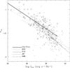Fig. 3 αox as a function of the 2500 Å specific luminosity LUV, for samples A (circles and triangles) and B (circles) and for the sample of Paper I (dots). Triangles refer to radio-loud sources, circles to radio-quiet and radio-unclassified sources. Linear fits are shown for the present work, and are marked for previous works G10 (Grupe et al. 2010), V10 (Paper I), J07 (Just et al. 2007), G08 (Gibson et al. 2008).

3.1. Dispersion

We define the residuals 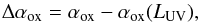$\mathrm{\Delta }{\mathit{\alpha }}_{\mathrm{ox}}\mathrm{=}{\mathit{\alpha }}_{\mathrm{ox}}\mathrm{-}{\mathit{\alpha }}_{\mathrm{ox}}\mathrm{\left(}{\mathit{L}}_{\mathrm{UV}}\mathrm{\right)}\mathit{,}$(9)adopting Eq. (8) as our reference α_ox(L_UV) relation. The standard deviation of our distribution of the residuals is σ = 0.124 for sample A and σ = 0.117 for sample B. The dispersion in our Δα_ox distribution is of the same order as those obtained in some studies based on non-simultaneous X-ray and UV data. Indeed, it is lower than those found by Strateva et al. (2005, e.g.) (0.14) and by Young et al. (2010) (0.16), but slightly higher than that evaluated by Gibson et al. (2008) (0.10). Values found in previous simultaneous studies are also of the same order, e.g. our XMM-Newton sample of Paper I (0.12), and the small clean catalogue by Wu et al. (2012) (0.12). Hence we confirm our conclusion of Paper I, that non-simultaneity of X-ray and UV measurements, which we call artificial α_ox variability, is not the main contributor to the dispersion of the residuals Δα_ox. Wu et al. (2012) reached the opposite conclusion, but they compared their results only with those of Just et al. (2007) (0.15). Non-simultaneity would lead to an artificial change of α_ox caused by the sole change of the X-ray flux in the time elapsed from the optical measurement, or vice versa. An average change of 15–30% in a few years would apply for the optical case (see e.g. Wilhite et al. 2008; MacLeod et al. 2012), and 40–50% for the X-ray case (Markowitz & Edelson 2004; Vagnetti et al. 2011). Applying Eq. (1), this would translate into an α_ox artificial change of ≲0.07. On the other hand, as we have shown in Paper I, and as we will discuss in more detail below, there is a sizable intrinsic α_ox variability that we estimate to be ~0.07, large enough to provide a significant contribution, at least of the same order as the artificial variability, even when the latter is removed by simultaneous X/UV measurements.

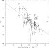Fig. 4 Tracks of individual sources of sample B in the plane αox − LUV. Connected segments show the tracks of multi-epoch sources, while open circles represent the average values of the same sources, which are labelled with their serial numbers as in Table 1. Objects with single-epoch measurements are represented by dots. The straight line is the adopted αox − LUV relation, Eq. (8).

3.2. Tracks of individual sources

Multi-epoch information is available for 68/86 sources of sample A and for 61/77 sources of sample B. We show in Fig. 4 the tracks of individual sources in the α_ox − L_UV plane for sample B. Strong variations in α_ox are clearly occurring for many sources, and most tracks appear to be almost vertical, suggesting the occurrence of strong changes in X-rays, and/or weak changes in L_UV. This is confirmed by the histograms of the individual variability dispersions of log L_UV and log L_X for multi-epoch sources, shown in Fig. 5. The variations occur on various time scales from days to years, therefore a better evaluation of the variability properties will be made in the next section. We note, however, that some factors could affect this apparent behaviour, e.g. the presence of a large number of narrow line Seyfert 1 (NLS1) nuclei, which are known to have strong X-ray variability (e.g. Leighly 1999) and moderate optical variability (e.g. Ai et al. 2010). We instead corrected for the effect of the other important factor, dilution of the optical variability by the host galaxy.

Fig. 5 Histograms of the individual variability dispersions of log LUV and log LX for multi-epoch sources: shaded histogram, UV; empty histogram, X-ray.

3.3. Effect of the host galaxy

Although we have subtracted host galaxy luminosities in Sect. 2.1, it is useful to discuss the possible effects of their contributions, for comparison with the literature. Wilkes et al. (1994) first pointed out that contamination by host galaxy starlight could affect the α_ox − L_UV relation, and that excluding the lowest luminosity AGNs would cause a marginal steepening of the relation. G10 mentioned the possibility that the measured magnitudes are affected by a contribution of the host galaxy starlight within the UVOT standard extraction radius of 5 arcsec, estimating this effect to be important for a few extreme cases like Mark 493. Wu et al. (2012) analysed a large sample of quasars on wide L and z intervals, and pointed out that their α_ox − L_UV slope decreases from − 0.16 to − 0.14 when the G10 sample is added, arguing that the difference in slopes is likely caused by host galaxy contamination at low redshift. Lusso et al. (2010) modelled the optical spectrum as a combination of AGN and galaxy components, L_ν = Aν^-0.5 + Gν^-3, and estimated the galaxy contribution from the measure of the optical spectral index. This enabled the authors to correct their α_ox − L_UV relation, which results in a steepening from − 0.154 to −0.197. Xu (2011) analysed a sample of low-luminosity AGNs, including 28 local Seyfert galaxies and 21 low-ionization nuclear emission-line regions (LINERs), with L_UV luminosities in the range 10²²−10^27.7 erg s^-1 Hz^-1. The author took the nuclear magnitudes directly observed by Ho & Peng (2001) with the Hubble Space Telescope, or estimated from H_β luminosity, and found for the relation α_ox − L_UV a steeper slope (− 0.134) than G10, but similar to our result of Eq. (8) and to that found by Just et al. (2007) for higher luminosity AGNs.

While Eq. (8) is corrected for galactic dilution, we computed the same relation for uncorrected (diluted) luminosities as well, α_ox = ( − 0.103 ± 0.016)log L_UV + (1.679 ± 0.472), which is flatter. The dilution effect is shown in Fig. 6, where some of the low-luminosity sources are shifted towards higher L_UV and lower α_ox, along lines with slope − 0.384, according to Eq. (1). This slope is higher than the anti-correlation slope, especially in the low-luminosity range, and determines a flattening of the observed anti-correlation.

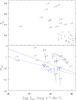Fig. 6 Effect of the dilution by the host galaxy. Upper panel: galactic fraction fg as a function of the UV luminosity; sources with fg > 30% are represented by circles and are numbered, sources with fg < 30% are shown as dots. Lower panel: the αox − LUV relation before (blue) and after (black) correction for galaxy dilution. Only the most diluted sources are shown, all shifted along lines with slope −0.384, by amounts increasing with fg. Sources 44 and 89 have a reduced number of epochs after correction, due to the requirement that the SED contains at least four UVOT points, as discussed in Sect. 2.1.

4. Structure functions

We now computed for the 59 multi-epoch sources of sample B an ensemble structure function (SF) to describe the variability of α_ox as a function of the rest-frame time lag τ. We define this as in di Clemente et al. (1996), and in agreement with the procedure used in Paper I: $\mathit{S}{\mathit{F}}_{\mathit{\alpha }}\mathrm{\left(}\mathit{\tau }\mathrm{\right)}\mathrm{=}\sqrt{\mathit{\pi }\mathit{/}\mathrm{2}}\hspace{0.17em}\mathrm{⟨}\mathrm{\left|}{\mathit{\alpha }}_{\mathrm{ox}}\mathrm{\right(}\mathit{t}\mathrm{+}\mathit{\tau }\mathrm{)}\mathrm{-}{\mathit{\alpha }}_{\mathrm{ox}}\mathrm{(}\mathit{t}\mathrm{\left)}\mathrm{\right|}\mathrm{⟩}\hspace{0.17em}\mathit{,}$(10)where t and t + τ are two epochs, in the rest-frame, at which α_ox is determined. The factor $\sqrt{\mathit{\pi }\mathit{/}\mathrm{2}}$ is introduced³ to normalise the SF to the rms value in the case of a Gaussian distribution, and the angular brackets indicate the ensemble average over appropriate bins of time lag.

The SF, displayed in Fig. 7, shows an average increasing behaviour. Maximum variations are ~0.073 at ~1 month rest-frame, and can be compared with the total dispersion in the residuals, σ ~ 0.117.

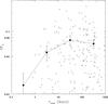Fig. 7 Structure function of αox(t) vs. the rest-frame time lag for sample B. The crosses represent the variations of individual sources for any pair of epochs. The filled circles connected by continuous lines represent the binned ensemble structure function.

As found in Paper I, variability in α_ox for individual sources accounts for a large part of the observed dispersion around the average α_ox − L_UV correlation. We call this intra-source dispersion, while the scatter of the time-average of α_ox values for individual sources constitutes the inter-source dispersion. The overall variance is then 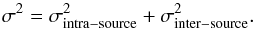${\mathit{\sigma }}^{\mathrm{2}}\mathrm{=}{\mathit{\sigma }}_{\mathrm{intra}\mathrm{-}\mathrm{source}}^{\mathrm{2}}\mathrm{+}{\mathit{\sigma }}_{\mathrm{inter}\mathrm{-}\mathrm{source}}^{\mathrm{2}}\mathit{.}$(11)Inserting the values 0.073 and 0.117 that we obtained for the intra-source and total dispersions, into Eq. (11) indicates a ~40% contribution of the intra-source dispersion to the total variance σ², similar to Paper I.

4.1. X-ray SF

It is also useful to compute separate structure functions (SF) for the X-ray and optical variations, to compare the variability properties of this sample with previous analyses. We therefore define $\mathit{S}{\mathit{F}}_{\mathrm{X}}\mathrm{\left(}\mathit{\tau }\mathrm{\right)}\mathrm{=}\sqrt{\mathit{\pi }\mathit{/}\mathrm{2}}\hspace{0.17em}\mathrm{⟨}\mathrm{\left|}\log {\mathit{F}}_{\mathit{X}}\mathrm{\right(}\mathit{t}\mathrm{+}\mathit{\tau }\mathrm{)}\mathrm{-}\log {\mathit{F}}_{\mathit{X}}\mathrm{(}\mathit{t}\mathrm{\left)}\mathrm{\right|}\mathrm{⟩}\mathit{,}$(12)where F_X is the X-ray flux in the observed 0.2–2 keV band. This is similar to the definition introduced by us (Vagnetti et al. 2011), except that we here omit the subtraction of the contribution due to photometric noise, which turns out to be negligible in this case (σ_n ~ 0.01).

The structure function, shown in Fig. 8, represents a variability of ≳0.2 at ~1 yr in the logarithm, or ~60%. This can be compared with the SF obtained by us from the XMM-Newton serendipitous source catalogue (Vagnetti et al. 2011), which has similar levels of variability at all timescales. The observed X-ray band in that case is 0.5–4.5 keV, which translates into ~1–11 keV for the higher redshifts of that sample. The luminosities are also different, but the same variability is found for the lower luminosity sources in the Vagnetti et al. (2011) sample, which are comparable to the sources in the present sample. For low-redshift AGNs, most authors use normalised excess variance or fractional variability, and no structure function analyses are available. The energy bands are also usually harder. For example, Markowitz & Edelson (2004) found a fractional variability F_var between 10% and 70% for 55 Seyfert 1 AGNs at months-to-years timescale in the 2–4 keV band. Chitnis et al. (2009) found an average long-term fractional variability ~60% in the 1.5–3 keV band for ~30 Seyferts. No direct comparisons are available in the 0.2–2 keV band; energy-dependent analyses (Gierliński & Done 2006; Arévalo et al. 2008) report a peak of variability around 1–2 keV for a few Seyferts, with decreasing variability both at lower and higher energies, although different behaviours are found for other sources. With these limitations, our SF in Fig. 8 compares reasonably well with other results for similar AGN populations.

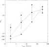Fig. 8 Binned ensemble structure function of the X-ray flux in the 0.2–2 keV band vs. the rest-frame time lag. Continuous line: whole sample B; dotted line: NLS1; dashed line: BLS1.

4.2. Optical/UV SF

Here, we define $\mathit{S}{\mathit{F}}_{\mathit{O}}\mathrm{\left(}\mathit{\tau }\mathrm{\right)}\mathrm{=}\sqrt{\mathit{\pi }\mathit{/}\mathrm{2}}\hspace{0.17em}\mathrm{⟨}\mathrm{\left|}\mathit{m}\mathrm{\right(}\mathit{t}\mathrm{+}\mathit{\tau }\mathrm{)}\mathrm{-}\mathit{m}\mathrm{(}\mathit{t}\mathrm{\left)}\mathrm{\right|}\mathrm{⟩}\mathit{,}$(13)where m is the apparent magnitude in any of the UVOT bands. We omitted noise subtraction in this case as well. We stress that optical variabilities measured through Eq. (13) differ from the X-ray variabilities measured through Eq. (12) by the factor 2.5 introduced by the magnitudes, that are usually adopted in optical studies.

The result is shown in Fig. 9, upper panel, for the six UVOT bands, and represents a variability of ~0.3–0.4 mag at ~1 yr. The values of our SFs can be compared with many other SF analyses, although most of them refer to quasars at higher redshifts. For example, Vanden Berk et al. (2004) found SF ~ 0.2 − 0.15 in the SDSS gri bands, and Wilhite et al. (2008)SF ~ 0.3 − 0.15 in the ugriz bands, which scan an overall rest-frame range ~1400 − 3600 Å at ⟨ z ⟩  ~ 1.5. MacLeod et al. (2012) found SF ≲ 0.2 in the rest-frame interval 2000–3000 Å. For the low-redshift AGNs of the present sample, the above λ intervals are well covered by the four harder UVOT bands, UVW2, UVM2, UVW1, U, where our SFs are ≳0.3 mag. The variability of our sample is then slightly higher than the variability of the comparison samples. This is also due to the lower luminosity of our sources, however, and to the well-known fact that variability decreases with luminosity (e.g., as L^-0.246 following Vanden Berk et al. 2004). Therefore, we extracted from our sample B a subsample of sources with ⟨ L_UV ⟩  ≥ 10²⁹ erg s^-1 Hz^-1, well-matched with the luminosities of the Vanden Berk et al. (2004) and Wilhite et al. (2008) samples. The SFs for this subsample, shown in the middle panel of Fig. 9, amount to ≲0.2 mag at 1 yr, similar to the comparison samples.

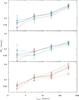Fig. 9 UV/optical structure function. Upper panel: whole sample B, UVOT filters UVW2 (black), UVM2 (blue), UVW1 (cyan), U (green), B (magenta), V (red). Middle panel: subsample with LUV ≥ 1029 erg s-1 Hz-1, same colour-code. Lower panel: NLS1 (dotted lines), BLS1 (dashed lines), whole sample B (continuous lines). Only the UVW2 filter (black) and the V filter (red) are shown.

4.3. NLS1s

The presence of several NLS1 AGNs in our sample (28 NLS1 among 61 multi-epoch sources of sample B) gives us the opportunity to measure their variability compared with broad line Seyfert 1 galaxies (BLS1). NLS1 are known to be strongly X-ray variable for timescales ≲1 day (e.g. Leighly 1999), and have been suggested to be strongly variable even at longer timescales (Horikawa et al. 2001). We show in Fig. 8 the X-ray SF of NLS1 (dotted line) and BLS1 (dashed line), compared with the overall behaviour of sample B (continuous line). Clearly, NLS1 vary more than the average, and BLS1 less than the average, on timescales shorter than a few months, while there is no such indication for a lag of ~1 yr.

We show in the lower panel of Fig. 9 the optical/UV SFs of our NLS1 (dotted lines) and BLS1 (dashed lines), together with the overall sample B (continuous lines), for the extremal UVOT filters UVW2 (black) and V (red). In both filters, NLS1 are less variable than the average, and BLS1 more variable. Our result confirms previous findings of a weak optical variability of NLS1 (e.g. Ai et al. 2010).

5. Discussion

This paper is the second of a series aiming to quantify the contribution of X-ray and UV variability to the dispersion of the α_ox − L_UV anti-correlation. It is confirmed that this contribution is significant (~40% of the total variance for this sample), while the artificial α_ox variability, present in many analyses because of the non-simultaneity of X-ray and UV/optical observations, turns out to be less important in the sense that it is surpassed by the intrinsic α_ox variability. Indeed, strong X-ray and/or UV changes occur for individual sources: while these variations could in principle occur with minor changes of the X-ray/UV ratio, the strong α_ox variations (measured by simultaneous X-ray/UV observations) demonstrate that this is not the case.

Stronger variations occur in the X-rays than in UV. While this behaviour could be affected by the presence of many NLS1, which are strongly variable in X-rays, we have shown that the average variability properties of the analysed sample do not suggest a special effect of this factor.

We also discussed the effect of host galaxy dilution on the slope of the α_ox − L_UV anti-correlation. We showed that the effect is significant for a limited number of low-luminosity sources, still producing a significant flattening of the relation. Even when corrected for the dilution effect, the α_ox − L_UV relation remains flatter than those found at high luminosities by Gibson et al. (2008) and by ourselves (Paper I).

Interestingly, in the recent work by Sazonov et al. (2012), the authors evaluated corona luminosities for a sample of 68 Seyfert galaxies through hard X-ray observations by INTEGRAL and accretion disk luminosities through Spitzer observations of the radiation reprocessed by the torus in the mid-infrared, and estimated a disk/corona luminosity ratio approximately constant over two decades in luminosity. While this apparently would contradict the α_ox − L_UV anti-correlation, the authors argued that the 2500 Å luminosity L_UV is a good indicator of the accretion disk luminosity for quasars, but not for lower luminosity AGNs, which are expected to have smaller mass black holes, and hotter accretion disks, with emission peaked in the extreme UV, rather than in the near-UV. This would suggest that α_ox is nearly constant at low luminosities, but this indication is not supported by our findings, Eq. (8), nor by those of Xu (2011).

The variability of α_ox, measured by the SFs of Paper I and of the present paper, also gives information on the relation between disk and corona emissions and their variabilities. This relation is complex and includes many processes, e.g variable X-ray irradiation driving optical variations through variable heating of the internal parts of the disk on relatively short timescales, and Compton upscattering in the corona by UV/optical photons generated in the accretion disk and variable on longer timescales due to disk instabilities born in the outer parts of the disk and propagating inwards (e.g. Czerny 2006; Arévalo 2006). The SF of α_ox, shown in Fig. 7, increases with the time lag up to ~1 month, while in Paper I another increase at ~1 year was also present. These findings indicate the substantial contribution of the intermediate-long timescale variations, possibly generated in the outer parts of the accretion disk.

Another interesting aspect concerns the inter-source dispersion, i.e. the residual dispersion of the α_ox − L_UV relation after accounting for the effect of variability. This could be related to the dependence of α_ox on a second physical parameter, in addition to the primary dependence on luminosity. For example, both Lusso et al. (2010) and G10 found evidence of a decrease of α_ox with Eddington ratio. Moreover, Young et al. (2010) found a significant partial anti-correlation with the Eddington ratio when the dependence on L_UV is accounted for; the significance increases if the X-ray energy in the α_ox definition is increased.

Another step in the investigation of the variability of α_ox would be a better temporal sampling of the simultaneous X-ray and optical observations. An appropriate strategy would be a multi-epoch survey of the same field with an X-ray/optical telescope such as XMM-Newton or Swift, and the opportunity is punctually offered by the XMM Deep survey in the Chandra Deep Field South (Comastri et al. 2011). We are preparing an analysis of the individual properties of α_ox variability for the brightest sources, which have simultaneous X-ray/optical multi-epoch information (Vagnetti et al, in preparation).

Online material

Acknowledgments

We thank Dirk Grupe for help in using his published data, and for suggestions and comments. We thank Maurizio Paolillo, Sara Turriziani, and Guido Risaliti for useful discussions. We thank the referee, who induced us to correcting for the host galaxy contamination. F.V. acknowledges hospitality by the University of Rome “La Sapienza”, during his sabbatical leave from the University of Rome “Tor Vergata”. This research has made use of data and/or software provided by the High Energy Astrophysics Science Archive Research Center (HEASARC), which is a service of the Astrophysics Science Division at NASA/GSFC and the High Energy Astrophysics Division of the Smithsonian Astrophysical Observatory. This research has made use of the NASA/IPAC Extragalactic Database (NED), which is operated by the Jet Propulsion Laboratory, California Institute of Technology, under contract with the National Aeronautics and Space Administration. No financial resources have been granted to this research by the University of Roma “Tor Vergata”.

References

All Tables

All Figures

	Fig. 1 Distribution of the sources in the LUV-z plane. Open circles: Swift sample; dots: XMM-Newton sample.
In the text

Fig. 2 Spectral energy distributions from the available UVOT data. Black lines refer to sources with data at a single epoch, while coloured lines refer to multi-epoch sources. Data from the same source are plotted with the same colour, but more sources are represented with the same colour. The continuous curve that covers the whole range of the plot is the average SED computed by Richards et al. (2006) for type 1 quasars from the SDSS.

In the text

Fig. 3 αox as a function of the 2500 Å specific luminosity LUV, for samples A (circles and triangles) and B (circles) and for the sample of Paper I (dots). Triangles refer to radio-loud sources, circles to radio-quiet and radio-unclassified sources. Linear fits are shown for the present work, and are marked for previous works G10 (Grupe et al. 2010), V10 (Paper I), J07 (Just et al. 2007), G08 (Gibson et al. 2008).

In the text

	Fig. 4 Tracks of individual sources of sample B in the plane αox − LUV. Connected segments show the tracks of multi-epoch sources, while open circles represent the average values of the same sources, which are labelled with their serial numbers as in Table 1. Objects with single-epoch measurements are represented by dots. The straight line is the adopted αox − LUV relation, Eq. (8).
In the text

	Fig. 5 Histograms of the individual variability dispersions of log LUV and log LX for multi-epoch sources: shaded histogram, UV; empty histogram, X-ray.
In the text

Fig. 6 Effect of the dilution by the host galaxy. Upper panel: galactic fraction fg as a function of the UV luminosity; sources with fg > 30% are represented by circles and are numbered, sources with fg < 30% are shown as dots. Lower panel: the αox − LUV relation before (blue) and after (black) correction for galaxy dilution. Only the most diluted sources are shown, all shifted along lines with slope −0.384, by amounts increasing with fg. Sources 44 and 89 have a reduced number of epochs after correction, due to the requirement that the SED contains at least four UVOT points, as discussed in Sect. 2.1.

In the text

	Fig. 7 Structure function of αox(t) vs. the rest-frame time lag for sample B. The crosses represent the variations of individual sources for any pair of epochs. The filled circles connected by continuous lines represent the binned ensemble structure function.
In the text

	Fig. 8 Binned ensemble structure function of the X-ray flux in the 0.2–2 keV band vs. the rest-frame time lag. Continuous line: whole sample B; dotted line: NLS1; dashed line: BLS1.
In the text

	Fig. 9 UV/optical structure function. Upper panel: whole sample B, UVOT filters UVW2 (black), UVM2 (blue), UVW1 (cyan), U (green), B (magenta), V (red). Middle panel: subsample with LUV ≥ 1029 erg s-1 Hz-1, same colour-code. Lower panel: NLS1 (dotted lines), BLS1 (dashed lines), whole sample B (continuous lines). Only the UVW2 filter (black) and the V filter (red) are shown.
In the text

References

- Ai, Y. L., Yuan, W., Zhou, H. Y., et al. 2010, ApJ, 716, L31 [NASA ADS] [CrossRef] [Google Scholar]
- Arévalo, P. 2006, in VI Microquasar Workshop: Microquasars and Beyond, PoS(MQW6)032 [Google Scholar]
- Arévalo, P., McHardy, I. M., Markowitz, A., et al. 2008, MNRAS, 387, 279 [NASA ADS] [CrossRef] [Google Scholar]
- Bentz, M. C., Peterson, B. M., Netzer, H., Pogge, R. W., & Vestergaard, M. 2009, ApJ, 697, 160 [Google Scholar]
- Brandt, W. N., Laor, A., & Wills, B. J. 2000, ApJ, 528, 637 [NASA ADS] [CrossRef] [Google Scholar]
- Chitnis, V. R., Pendharkar, J. K., Bose, D., et al. 2009, ApJ, 698, 1207 [NASA ADS] [CrossRef] [Google Scholar]
- Comastri, A., Ranalli, P., Iwasawa, K., et al. 2011, A&A, 526, L9 [NASA ADS] [CrossRef] [EDP Sciences] [Google Scholar]
- Czerny, B. 2006, in ASP Conf. Ser. 360, eds. C. M. Gaskell, I. M. McHardy, B. M. Peterson, & S. G. Sergeev, 265 [Google Scholar]
- di Clemente, A., Giallongo, E., Natali, G., Trevese, D., & Vagnetti, F. 1996, ApJ, 463, 466 [NASA ADS] [CrossRef] [Google Scholar]
- Ganguly, R., Brotherton, M. S., Arav, N., et al. 2007, AJ, 133, 479 [NASA ADS] [CrossRef] [Google Scholar]
- Gibson, R. R., Brandt, W. N., & Schneider, D. P. 2008, ApJ, 685, 773 [NASA ADS] [CrossRef] [Google Scholar]
- Gierliński, M., & Done, C. 2006, MNRAS, 371, L16 [NASA ADS] [CrossRef] [Google Scholar]
- Green, P. J., & Mathur, S. 1996, ApJ, 462, 637 [NASA ADS] [CrossRef] [Google Scholar]
- Grupe, D., Thomas, H.-C., & Beuermann, K. 2001, A&A, 367, 470 [NASA ADS] [CrossRef] [EDP Sciences] [Google Scholar]
- Grupe, D., Komossa, S., Leighly, K. M., & Page, K. L. 2010, ApJS, 187, 64 [NASA ADS] [CrossRef] [Google Scholar]
- Ho, L. C., & Peng, C. Y. 2001, ApJ, 555, 650 [NASA ADS] [CrossRef] [Google Scholar]
- Horikawa, T., Hayashida, K., & Katayama, H. 2001, in New Century of X-ray Astronomy, eds. H. Inoue, & H. Kunieda, ASP Conf. Ser., 251, 360 [Google Scholar]
- Just, D. W., Brandt, W. N., Shemmer, O., et al. 2007, ApJ, 665, 1004 [Google Scholar]
- Kellermann, K. I., Sramek, R., Schmidt, M., Shaffer, D. B., & Green, R. 1989, AJ, 98, 1195 [NASA ADS] [CrossRef] [Google Scholar]
- Kinney, A. L., Bohlin, R. C., Blades, J. C., & York, D. G. 1991, ApJS, 75, 645 [NASA ADS] [CrossRef] [Google Scholar]
- Leighly, K. M. 1999, ApJS, 125, 297 [NASA ADS] [CrossRef] [Google Scholar]
- Lusso, E., Comastri, A., Vignali, C., et al. 2010, A&A, 512, A34 [NASA ADS] [CrossRef] [EDP Sciences] [Google Scholar]
- MacLeod, C. L., Ivezić, Ž., Sesar, B., et al. 2012, ApJ, 753, 106 [NASA ADS] [CrossRef] [Google Scholar]
- Markowitz, A., & Edelson, R. 2004, ApJ, 617, 939 [NASA ADS] [CrossRef] [Google Scholar]
- Pettini, M., & Boksenberg, A. 1985, ApJ, 294, L73 [NASA ADS] [CrossRef] [Google Scholar]
- Poole, T. S., Breeveld, A. A., Page, M. J., et al. 2008, MNRAS, 383, 627 [NASA ADS] [CrossRef] [Google Scholar]
- Press, W. H., Teukolsky, S. A., Vetterling, W. T., & Flannery, B. P. 1992, Numerical recipes in FORTRAN. The art of scientific computing [Google Scholar]
- Richards, G. T., Lacy, M., Storrie-Lombardi, L. J., et al. 2006, ApJS, 166, 470 [NASA ADS] [CrossRef] [Google Scholar]
- Richards, G. T., Kruczek, N. E., Gallagher, S. C., et al. 2011, AJ, 141, 167 [NASA ADS] [CrossRef] [Google Scholar]
- Roming, P. W. A., Kennedy, T. E., Mason, K. O., et al. 2005, Space Sci. Rev., 120, 95 [NASA ADS] [CrossRef] [Google Scholar]
- Roming, P. W. A., Gronwall, C., van den Berk, D. E., Page, M. J., & Boyd, P. T. 2009, Ap&SS, 320, 203 [NASA ADS] [CrossRef] [Google Scholar]
- Sazonov, S., Willner, S. P., Goulding, A. D., et al. 2012, ApJ, 757, 181 [NASA ADS] [CrossRef] [Google Scholar]
- Sramek, R. A., & Weedman, D. W. 1980, ApJ, 238, 435 [NASA ADS] [CrossRef] [Google Scholar]
- Steffen, A. T., Strateva, I., Brandt, W. N., et al. 2006, AJ, 131, 2826 [NASA ADS] [CrossRef] [Google Scholar]
- Strateva, I. V., Brandt, W. N., Schneider, D. P., Van den Berk, D. G., & Vignali, C. 2005, AJ, 130, 387 [NASA ADS] [CrossRef] [Google Scholar]
- Sulentic, J. W., Dultzin-Hacyan, D., Marziani, P., et al. 2006, Rev. Mex. Astron. Astrofis., 42, 23 [NASA ADS] [Google Scholar]
- Thomas, H.-C., Beuermann, K., Reinsch, K., et al. 1998, A&A, 335, 467 [NASA ADS] [Google Scholar]
- Turnshek, D. A., & Grillmair, C. J. 1986, ApJ, 310, L1 [NASA ADS] [CrossRef] [Google Scholar]
- Turnshek, D. A., Monier, E. M., Sirola, C. J., & Espey, B. R. 1997, ApJ, 476, 40 [NASA ADS] [CrossRef] [Google Scholar]
- Vagnetti, F., Turriziani, S., Trevese, D., & Antonucci, M. 2010, A&A, 519, A17 [NASA ADS] [CrossRef] [EDP Sciences] [Google Scholar]
- Vagnetti, F., Turriziani, S., & Trevese, D. 2011, A&A, 536, A84 [NASA ADS] [CrossRef] [EDP Sciences] [Google Scholar]
- Van den Berk, D. E., Wilhite, B. C., Kron, R. G., et al. 2004, ApJ, 601, 692 [NASA ADS] [CrossRef] [Google Scholar]
- Voges, W., Aschenbach, B., Boller, T., et al. 1999, A&A, 349, 389 [NASA ADS] [Google Scholar]
- Watson, M. G., Schröder, A. C., Fyfe, D., et al. 2009, A&A, 493, 339 [NASA ADS] [CrossRef] [EDP Sciences] [Google Scholar]
- Wilhite, B. C., Brunner, R. J., Grier, C. J., Schneider, D. P., & van den Berk, D. E. 2008, MNRAS, 383, 1232 [NASA ADS] [CrossRef] [Google Scholar]
- Wilkes, B. J., Tananbaum, H., Worrall, D. M., et al. 1994, ApJS, 92, 53 [NASA ADS] [CrossRef] [Google Scholar]
- Worrall, D. M., Tananbaum, H., Giommi, P., & Zamorani, G. 1987, ApJ, 313, 596 [NASA ADS] [CrossRef] [Google Scholar]
- Wu, J., Van den Berk, D., Grupe, D., et al. 2012, ApJS, 201, 10 [NASA ADS] [CrossRef] [Google Scholar]
- Xu, Y.-D. 2011, ApJ, 739, 64 [NASA ADS] [CrossRef] [Google Scholar]
- Young, M., Elvis, M., & Risaliti, G. 2010, ApJ, 708, 1388 [NASA ADS] [CrossRef] [Google Scholar]
- Zamorani, G., Henry, J. P., Maccacaro, T., et al. 1981, ApJ, 245, 357 [NASA ADS] [CrossRef] [Google Scholar]