| Issue |
A&A
Volume 550, February 2013
|
|
|---|---|---|
| Article Number | A59 | |
| Number of page(s) | 11 | |
| Section | Astronomical instrumentation | |
| DOI | https://doi.org/10.1051/0004-6361/201220429 | |
| Published online | 28 January 2013 | |
Self-calibration: an efficient method to control systematic effects in bolometric interferometry
1
APC, Astroparticule et Cosmologie, Université Paris Diderot,
Bâtiment Condorcet, 10 rue Alice Domon et Léonie
Duquet,
75205
Paris Cedex 13,
France
e-mail: This email address is being protected from spambots. You need JavaScript enabled to view it.
2
Turing-Solutions, 25 rue Dauphine, 75006
Paris,
France
Received:
21
September
2012
Accepted:
4
December
2012
Abstract
Context. The QUBIC collaboration is building a bolometric interferometer dedicated to the detection of B-mode polarization fluctuations in the cosmic microwave background.
Aims. We introduce a self-calibration procedure related to those used in radio-interferometry to control a wide range of instrumental systematic errors in polarization-sensitive instruments.
Methods. This procedure takes advantage of the need for measurements on redundant baselines to match each other exactly in the absence of systematic effects. For a given systematic error model, measuring each baseline independently therefore allows writing a system of nonlinear equations whose unknowns are the systematic error model parameters (gains and couplings of Jones matrices, for instance).
Results. We give the mathematical basis of the self-calibration. We implement this method numerically in the context of bolometric interferometry. We show that, for large enough arrays of horns, the nonlinear system can be solved numerically using a standard nonlinear least-squares fitting and that the accuracy achievable on systematic effects is only limited by the time spent on the calibration mode for each baseline apart from the validity of the systematic error model.
Key words: instrumentation: polarimeters / instrumentation: interferometers / cosmic background radiation / inflation / methods: data analysis
© ESO, 2013
1. Introduction
The quest for the B-mode of the polarization of the cosmic background is one of the scientific priorities of observational cosmology today. Observing this mode appears to be the most powerful way to constrain inflation models. However, detecting such a weak signal is a real experimental challenge. In addition to a high statistical sensitivity (a huge number of horns and bolometers required), future experiments will need excellent quality of foreground removal and unprecedented control of instrumental effects.
Currently, most projects are based on the experimental concept of an imager. A promising alternative technology is bolometric interferometry. This is the project of the QUBIC instrument (QUBIC collaboration 2010). A first module is planned for installation at the Franco-Italian Concordia Station in Dome C, Antarctica in 2014. The aim is to combine the advantages of an imager in terms of sensitivity with those of an interferometer in terms of controlling systematic effects. The statistical sensitivity of the QUBIC instrument is comparable to that of an imager with the same number of horns covering the same sky fraction. The full QUBIC instrument (six modules) will comprise three frequencies (97, 150, and 220 GHz) and aims to constrain, at the 90% confidence level, a tensor-to-scalar ratio of 0.01 with one year of data.
The aim of this article is to introduce a new method, specific to bolometric interferometry, called self-calibration, and to give an example of application with the QUBIC instrument. This method allows a wide range of instrumental systematic effects to be controlled.
This self-calibration technique is based on the redundancy of the receiver array (Wieringa 1991). It uses the need for redundant baselines of the interferometer to measure exactly the same quantity in the absence of systematic effects. For a real instrument, these measurements will be different because of systematics. The small differences can be used to calibrate parameters that characterize the instrument completely for each channel and estimate the instrumental errors.
In the case of a bolometric interferometer, the square horn array will provide a large number of redundant baselines. In this way, a bolometric interferometer can be self-calibrated thanks to a calibration mode during which it will separately measure the nh(nh − 1)/2 baselines or a fraction of the nh(nh − 1)/2 baselines with nh the number of horns observing an external polarized source.
This method is inspired by traditional interferometry (Pearson & Readhead 1984) where signal phases are often lost due to atmospheric turbulence. Standard calibration procedures exist in radio-interferometry and are similar to those used for imaging techniques based on observations of an unresolved source whose flux is assumed to be known. We emphasize that the word self-calibration refers, by opposition, to a procedure in which no knowledge of the observed source is required (most of the time, the object which is scientifically studied is itself used as the calibration source). Most of these self-calibration techniques are based on the evaluation of so-called closure quantities phases or amplitudes. A set of unknown phases can, for instance, be iteratively reconstructed by forming quantities where they are nullified (the product of the three visibilities that can be formed with three antennas). The use of redundant baselines for calibration is in contrast rather uncommon in radio-interferometry (see Wieringa 1991; Noordam & de Bruyn 1982). This comes from most radio-interferometers having very few redundant baselines achieve very high angular resolution, it is indeed better to arrange a given number of antennas in order to optimize the uv-plane sampling, rather than to maximize redundancy.
A new kind of all-digital radio-interferometer the “omniscope”, dedicated to 21 cm observations, has recently been proposed by Tegmark & Zaldarriaga (2009; 2012); its concept can be summarized by the following five steps:
-
1)
signals collected by antennas are digitized right afteramplification,
-
2)
a temporal fast Fourier transform (FFT) is performed in order to split them into frequency subbands,
-
3)
a spatial FFT is performed on each subband set,
-
4)
the square modulus of the FFT result is computed,
-
5)
an inverse spatial FFT is performed to recover the visibilities.
There are conceptual similarities with the bolometric interferometer concepts, since in this instrument, steps two and three are performed in an analogical way by the beam combiner and the bolometers, respectively. Because antennas have to be located on a grid in order for the FFTs to be performed, an omniscope will possess many redundant baselines, and Liu et al. (2010) have shown how this allows self-calibrating the complex gains of the antennas. In both cases (standard radio-interferometer or omniscope), the aim is to calibrate the complex gains of the antennas and there is actually a mathematical trick to get a linear system of equations from which these gains can be obtained. The self-calibration procedure explained in this paper is inspired by methods used in the paper of Liu et al. (2010) even if the design of the QUBIC instrument is different.
This paper is organized as follows. Section 2 introduces the self-calibration method with the Jones matrix formalism and the Mueller matrix formalism for radio-interferometry and the omniscope. We show in Sect. 3 how the procedure can be applied to the QUBIC bolometric interferometer, and finally we describe the possible self-calibration algorithm and its results.
2. General principle
2.1. Instrumental systematics modelization with Jones matrices
In this section, we use the notation proposed by (O’Dea et al. 2007). With the electric field of an incident radiation at a frequency
φ defined as ![Mathematical equation: \hbox{$\mathbb{R}[{\overrightarrow{E}{\rm e}^{-{\rm i}\phi t}}]$}](/articles/aa/full_html/2013/02/aa20429-12/aa20429-12-eq4.png) , and
choosing two basis vectors
, and
choosing two basis vectors  and
and  orthogonal to the direction of propagation
  ,
all the statistical information is encoded in the coherence
matrix C
,
all the statistical information is encoded in the coherence
matrix C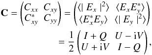 (1)where
Ex,
Ey are complex amplitudes of the
transverse electric field
(1)where
Ex,
Ey are complex amplitudes of the
transverse electric field  and I, Q, U, and V
are the Stokes parameters.
and I, Q, U, and V
are the Stokes parameters.
The propagation of an incident radiation
through a receiver can be described by a Jones matrix J such that
the electric field after passing through the receiver
 is
is  (2)where
the Jones matrix J is a 2 × 2 complex matrix. It describes how
the instrument linearly transforms the two-dimensional vector representing the incoming
radiation field
into the two-dimensional vector of the outgoing field
.
(2)where
the Jones matrix J is a 2 × 2 complex matrix. It describes how
the instrument linearly transforms the two-dimensional vector representing the incoming
radiation field
into the two-dimensional vector of the outgoing field
.
For an instrument with several components, the Jones matrix is the product of the Jones
matrices for each component. For example, the ideal Jones matrix for an instrument in
which the incident radiation passing through a rotating half-wave plate before propagating
through the horns is 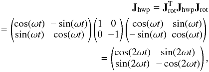 (3)where
ω is the angular velocity of the half-wave plate,
Jrot the rotation matrix and
Jhwp the ideal Jones matrix of the half-wave plate.
(3)where
ω is the angular velocity of the half-wave plate,
Jrot the rotation matrix and
Jhwp the ideal Jones matrix of the half-wave plate.
After passing through the receiver, ideal orthogonal linear detectors measure the power
in two components 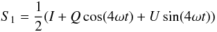
 To model systematic
errors within a polarization-sensitive interferometer, the Jones matrix can be described
by introducing diagonal terms: the complex gain parameters
gx and
gy and non-diagonal terms: the complex
coupling parameters ex and
ey associated to the orthogonal
polarizations
To model systematic
errors within a polarization-sensitive interferometer, the Jones matrix can be described
by introducing diagonal terms: the complex gain parameters
gx and
gy and non-diagonal terms: the complex
coupling parameters ex and
ey associated to the orthogonal
polarizations 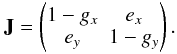 (4)Systematic errors arising
from the half-wave plate and from the square horn array can be modeled by
(4)Systematic errors arising
from the half-wave plate and from the square horn array can be modeled by
-
1.
a Jones matrix for the half-wave plate
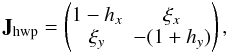 (5)
(5) -
2.
a Jones matrix for the horn i with

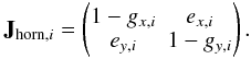 (6)
(6)
propagated through the half-wave plate and the horn i becomes
 (7)
(7)
2.2. Instrumental systematics modelisation with Mueller matrix
The Jones matrix expresses the transformation of the electric field in the x and y-directions and the Mueller matrix describes how the different polarization states transform. The Jones matrix is a 2 × 2 matrix, whereas the Mueller matrix is a 4 × 4 matrix. The 4 × 4 Mueller matrix can thus be written as the direct product of the 2 × 2 Jones matrices.
We calculate the tensor product of the outgoing field given by Eq. (2) 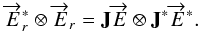 (8)In general, the
direct product
(8)In general, the
direct product  gives the vector
 defined as
 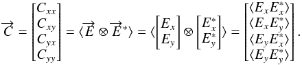 (9)With Eq. (8), one can write the transmission of the
electric field through an instrument described by its Jones matrix using the vector
of this electric field using the matrix direct product1
(9)With Eq. (8), one can write the transmission of the
electric field through an instrument described by its Jones matrix using the vector
of this electric field using the matrix direct product1
 (10)Accordingly Eq. (1), the polarization state of this electric
field can be described by the Stokes vector
(10)Accordingly Eq. (1), the polarization state of this electric
field can be described by the Stokes vector  defined by
 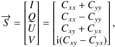 (11)where I,
Q, U, and V are the Stokes
parameters.
(11)where I,
Q, U, and V are the Stokes
parameters.
One can obtain the expression of the Stokes vector from the vector
defined in Eq. (9)  (12)where
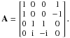 Substituting Eq. (12) into Eq. (10), it follows that the outgoing Stokes
vector
Substituting Eq. (12) into Eq. (10), it follows that the outgoing Stokes
vector  can be written as
 (13)where
M = A(J ⊗ J ∗ )A-1
is the Mueller matrix that describes how the Stokes parameters transform.
(13)where
M = A(J ⊗ J ∗ )A-1
is the Mueller matrix that describes how the Stokes parameters transform.
2.3. Polarized measurement equation with Mueller formalism
A polarization-sensitive interferometer measures the complex Stokes visibilities from all
baselines defined by the horns i and j in an array of
receivers ![Mathematical equation: \begin{equation} V_{ij}=\begin{pmatrix} V_{ij}^I \\[1mm] V_{ij}^Q \\[1mm] V_{ij}^U \\[1mm] V_{ij}^V \\ \end{pmatrix}. \label{eq:eq14} \end{equation}](/articles/aa/full_html/2013/02/aa20429-12/aa20429-12-eq56.png) (14)These vectors could
reduce to a scalar or a vector with 2, 3, or 4 elements depending on the Stokes parameters
the instrument is sensitive to. One can define
a = 1,2,3,4 as the
number of Stokes parameters the instrument allows to be measured.
(14)These vectors could
reduce to a scalar or a vector with 2, 3, or 4 elements depending on the Stokes parameters
the instrument is sensitive to. One can define
a = 1,2,3,4 as the
number of Stokes parameters the instrument allows to be measured.
The
nh(nh − 1)/2
baselines of the interferometer can be classified into sets
sβ of redundant baselines (same length,
same direction) indexed by β. In the absence of systematic errors, the
redundant visibilities should have exactly the same values 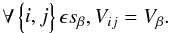 (15)For a real
instrument, however, redundant visibilites
(15)For a real
instrument, however, redundant visibilites  will not have exactly the same values because of systematic errors and statistical
(photon) noise, and one can write the following system of
a × nh(nh − 1)/2
complex equations
will not have exactly the same values because of systematic errors and statistical
(photon) noise, and one can write the following system of
a × nh(nh − 1)/2
complex equations 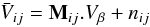 (16)where
nij are statistical noise terms and where
Mij are a kind of complex Mueller
matrices that reduce to the identity matrix for a perfect instrument:
(16)where
nij are statistical noise terms and where
Mij are a kind of complex Mueller
matrices that reduce to the identity matrix for a perfect instrument: 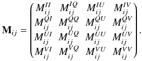 (17)The elements of these
matrices are not independent and can be expressed in terms of the diagonal and the
nondiagonal terms of the Jones matrix.
(17)The elements of these
matrices are not independent and can be expressed in terms of the diagonal and the
nondiagonal terms of the Jones matrix.
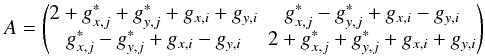
The first order Mueller matrix for a polarization sensitive experiment is
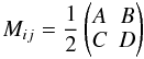 (18)with
 (19)
(19) (20)
(20) (21)
(21) (22)
(22)
3. Application to the QUBIC bolometric interferometer
3.1. Observables in bolometric interferometry
In this section, we derive the expression for the power received in the focal plane in the case of bolometric interferometry. The bolometric interferometer proposed with the QUBIC instrument (the QUBIC collaboration 2010) is the millimetric equivalent of the first interferometer dedicated to astronomy: the Fizeau interferometer − see Fig. 1 for the design of the QUBIC instrument.
The receptors are two arrays of nh horns: the primary and secondary horns back-to-back on a square grid behind the optical window of a cryostat. Filters and switches are placed in front and between the horn array. The switches will be only used during the calibration phase. The polarization of the incoming field is modulated using a half-wave plate located before the primary horns. This location of the half-wave plate avoids a leakage from the Stokes parameter I to the Stokes parameters Q and U if the half-wave plate has no inhomogeneities.
Signals are correlated together using an optical combiner. The interference fringe patterns arising from all pairs of horns, with a given angle, are focused to a single point on the focal plane. Finally, a polarizing grid splits the signal into x and y-polarizations, each being focused on a focal plane equipped with bolometers. These bolometers measure a linear combination of the Stokes parameters modulated by the rotating half-wave plate.
With an interferometer, the correlation between two receivers allows for direct access to the Fourier modes (visibilities) of the Stokes parameters I, Q, and U. In the case of a bolometric interferometer, the observable is the superposition of the fringes formed by the sky electric field passing through a large number of back-to-back horns and then focused on the detector plane array. The image on the focal plane of the optical combiner is the synthesized image, because only specific Fourier modes are selected by the receiving horns array. A bolometric interferometer is therefore a synthesized imager whose beam is the synthesized beam formed by the array of receiving horns.
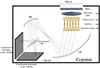 |
Fig. 1 Design of the QUBIC instrument. |
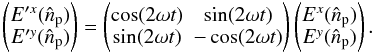
In the following section, we begin by defining the formalism for the QUBIC instrument in
an ideal case, that is to say, without systematics. The electric field
 passing through a half-wave plate that rotates at angular speed ω and
modulates the two orthogonal polarizations η ∈ {x,y}
becomes, as a function of the observed direction
passing through a half-wave plate that rotates at angular speed ω and
modulates the two orthogonal polarizations η ∈ {x,y}
becomes, as a function of the observed direction  ,
,
 (23)For an ideal instrument,
the electric field, after passing through the half-wave plate, collected by one horn
i located at
(23)For an ideal instrument,
the electric field, after passing through the half-wave plate, collected by one horn
i located at  for the polarization η ∈ {x,y} when all the primary
horns are looking at the same radiation field
for the polarization η ∈ {x,y} when all the primary
horns are looking at the same radiation field  as a function of the observed direction
and reaching the bolometer q at the direction
as a function of the observed direction
and reaching the bolometer q at the direction
 viewed from the optical center of the beam combiner is
 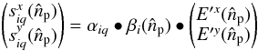 (24)where
 is the product matrix of the matrices αiq
and
is the product matrix of the matrices αiq
and  .
.
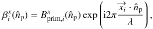
We have introduced the matrices  and αiq which characterize completely the
instrument. A matrix
is defined for each channel of pointings (p) and horns (i) and includes the primary beam
and αiq which characterize completely the
instrument. A matrix
is defined for each channel of pointings (p) and horns (i) and includes the primary beam
 , the horn position
and the direction of pointing
, the horn position
and the direction of pointing 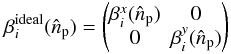 (25)with
 (26)and
 (27)A matrix
αiq is defined for each channel of horns
(i) and bolometers (q) and includes the geometrical phases induced by the beam combiner,
the beams of the secondary horns
(27)A matrix
αiq is defined for each channel of horns
(i) and bolometers (q) and includes the geometrical phases induced by the beam combiner,
the beams of the secondary horns  , and the
gain gq of the bolometer2
, and the
gain gq of the bolometer2 (28)with
![Mathematical equation: \begin{equation} \alpha_{iq}^{x}=g_q \int B^x_{\rm sec}(\hat{d}_q)\exp \left [ {\rm i}2\pi\frac{\overrightarrow{x}_i\cdot \hat{d}_q}{\lambda} \right ] J(\nu)\Theta(\hat{d}-\hat{d}_q){\rm d}\nu {\rm d}\hat{d}_q, \end{equation}](/articles/aa/full_html/2013/02/aa20429-12/aa20429-12-eq95.png) (29)and
(29)and
![Mathematical equation: \begin{equation} \alpha_{iq}^{y}=g_q \int B^y_{\rm sec}(\hat{d}_q)\exp \left[ {\rm i} 2\pi\frac{\overrightarrow{x}_i\cdot \hat{d}_q}{\lambda} \right ]J(\nu)\Theta(\hat{d}-\hat{d}_q){\rm d}\nu {\rm d}\hat{d}_q . \end{equation}](/articles/aa/full_html/2013/02/aa20429-12/aa20429-12-eq96.png) (30)The detector direction as
viewed from the optical center of the optical combiner is given by the unit vector
,
and λ is the wavelength of the instrument. The integrations are over the
surface of each individual bolometer modeled with the top-hat like function
(30)The detector direction as
viewed from the optical center of the optical combiner is given by the unit vector
,
and λ is the wavelength of the instrument. The integrations are over the
surface of each individual bolometer modeled with the top-hat like function
 3, and on bandwidths of the instrument
J(ν) with ν the frequency.
3, and on bandwidths of the instrument
J(ν) with ν the frequency.
We assume that there is no cross-polarization because the matrices
and αiq are written for an ideal case so that
there is no dependence on the direction of polarization. The power measured by one
polarized bolometer located at
in the focal plane of the beam combiner is then  (31)where
 is given in Eq. (24).
Without systematics, Eq. (31) can be
written as  (32)where the
synthesized beam
(32)where the
synthesized beam  for the detector
q is formed by the arrangement of the primary horns array as
for the detector
q is formed by the arrangement of the primary horns array as
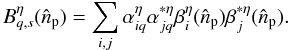 (33)The synthesized beam
depends on the sky direction
(33)The synthesized beam
depends on the sky direction  ,
so the synthesized image is the convolution of the sky and of the electric field through
the synthesized beam.
,
so the synthesized image is the convolution of the sky and of the electric field through
the synthesized beam.
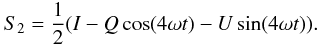
One can rewrite Eq. (31) to exhibit the
modulation of the polarization induced by the half-wave plate as  (34)where
ϵx = 1 for the polarization
x, ϵy = −1 for the
polarization y, and where
(34)where
ϵx = 1 for the polarization
x, ϵy = −1 for the
polarization y, and where  are the
synthesized images on the focal plane for each Stokes parameter
X = {I,Q,U}. The cosine and sine coefficients come
from the modulation induced by the rotating half-wave plate.
are the
synthesized images on the focal plane for each Stokes parameter
X = {I,Q,U}. The cosine and sine coefficients come
from the modulation induced by the rotating half-wave plate.
Systematic effects arising at any level of the detection can be modeled by associating a
Jones matrix to each horn i Jhorn,i
and a Jones matrix of the half-wave plate Jhwp. They
can be introduced as defined in Eq. (7),
and Eq. (24) becomes 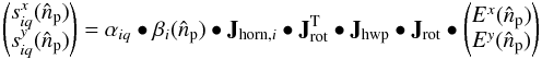 (35)where
 is the incident electric field,
Jhorn,i the Jones matrix of the
horn i, Jhwp the Jones matrix of the
half-wave plate, and Jrot the rotation matrix induced
by the rotation of the half-wave plate.
is the incident electric field,
Jhorn,i the Jones matrix of the
horn i, Jhwp the Jones matrix of the
half-wave plate, and Jrot the rotation matrix induced
by the rotation of the half-wave plate.
3.2. Self-calibration procedure
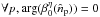
During the self-calibration mode, which is distinct from the ordinary data-taking mode, the instrument scans a polarized source and measures the nh(nh − 1)/2 synthesized images one by one from all baselines or only a fraction of them. In the QUBIC design, this can be achieved using switches located between the back-to-back horns. The switches are used as shutters that are operated independently for all channels and are only required during the calibration phase. One can modulate on/off a single pair of horns while leaving all the others open in order to access the synthesized images measured by each pair of horns alone. This procedure requires the knowledge of the individual primary beams of each horn. The maps of the primary beams can be obtained independently through scanning an external unpolarized source.
By repeating this with all baselines, all bolometers, and all directions of pointing, one can construct a system of equations whose unknowns are
-
1.
the complex coefficients
 ,
defined for each horn i, each bolometer q, and for
each polarization η which correspond to
4nhnq
parameters,
,
defined for each horn i, each bolometer q, and for
each polarization η which correspond to
4nhnq
parameters, -
2.
the horn location
(2nh parameters), -
3.
the direction of pointing
(2np parameters), -
4.
the complex horns systematic effects gx,i, gy,i, ex,i, ey,i defined for each horn i and for each polarization η (8nh parameters),
-
5.
the complex half-wave plate systematic effects hx, hy,ξx,ξy (8 parameters).
For an instrument with nh horns,
nq bolometers and for a scan
of np pointings, the number of unknowns is  (36)During the
self-calibration procedure, the number of constraints is given by the measurements, i.e.
the synthesized images. One has the
nh(nh − 1)/2
measured synthesized images for each
bolometer nq, each pointing
np, each Stokes parameter, and the two focal planes. The
number of constraints is given by
(36)During the
self-calibration procedure, the number of constraints is given by the measurements, i.e.
the synthesized images. One has the
nh(nh − 1)/2
measured synthesized images for each
bolometer nq, each pointing
np, each Stokes parameter, and the two focal planes. The
number of constraints is given by  (37)The problem becomes
easily overdetermined: for an instrument with nh = 9,
nq = 4, and
np = 10, the number of constraints is 8640 and the number of
unknowns is 262. It can be solved with a least squares algorithm.
(37)The problem becomes
easily overdetermined: for an instrument with nh = 9,
nq = 4, and
np = 10, the number of constraints is 8640 and the number of
unknowns is 262. It can be solved with a least squares algorithm.
The first module of the QUBIC instrument will consist of 400 primary horns and two 1024 element bolometer arrays. The number of constraints could be reduced if the self-calibration is performed not on the nh(nh − 1)/2 baselines but on a fraction of baselines. This is shown in the following.
Closing all the switches except two would actually dramatically change the thermal load
on the cryostat, which could affect the bolometric measurements. Fortunately, there is a
trick explained in Appendix A that allows  to be indirectly measured
while minimally changing the thermal load. One can show that
to be indirectly measured
while minimally changing the thermal load. One can show that  (38)where
 is the quantity measured by
a bolometer q when all the switches are open except the
i and j, and
is the quantity measured by
a bolometer q when all the switches are open except the
i and j, and  ,
,
 are the powers measured
when all the switches are open except respectively i or
j. Measuring these three terms therefore allows measuring
while keeping the thermal load
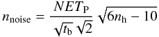
almost constant. However, this also increases the noise. The noise on each term is
therefore
are the powers measured
when all the switches are open except respectively i or
j. Measuring these three terms therefore allows measuring
while keeping the thermal load
almost constant. However, this also increases the noise. The noise on each term is
therefore 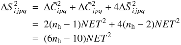 where
NET is the noise equivalent temperature of the bolometers, and
T the temperature of the 100% polarized source.
where
NET is the noise equivalent temperature of the bolometers, and
T the temperature of the 100% polarized source.
3.3. Numerical simulation
We have numerically implemented the method to check if the nonlinear system could be solved. We generate the instrument with a set of ideal parameters (horn locations, directions of pointing, primary and secondary beams, detector locations, etc.), and a set of parameters randomly corrupted by systematic errors (horn location errors, pointing errors, assymetries of beams, bolometer location errors, diagonal and nondiagonal terms of the Jones matrices, etc.). The widths of the random deviation of all corrupted parameters around their ideal value are given in Table 1. These values of corruption are independent Gaussian errors added to each parameter and each range of error is fixed according to the tolerance we impose on components.
Range for systematic errors for each parameter.
The primary beams  are assumed to be known
perfectly so their values are not varied in the simulation; however, the matrix
are assumed to be known
perfectly so their values are not varied in the simulation; however, the matrix
 varies as the horn locations
and the pointing directions
are unknowns of the system. In the simulation, the angular position of the half-wave plate
is drawn at random. A random angular position of the half-wave plate is given for each
measurement.
varies as the horn locations
and the pointing directions
are unknowns of the system. In the simulation, the angular position of the half-wave plate
is drawn at random. A random angular position of the half-wave plate is given for each
measurement.
To get a solvable system, one must add some normalization constraints for the
coefficients  and
, which do not change the
modeling of systematic errors. They mean that the self-calibration only allows for
relative calibration of these parameters. One can add
and
, which do not change the
modeling of systematic errors. They mean that the self-calibration only allows for
relative calibration of these parameters. One can add
-
1.
an absolute calibration of the global gain of the instrument,
 .
.
-
2.
a convention on the phase of the
coefficients,  .
A rotation of global phase φq applied
to the coefficients for one
bolometer q does not modify Eqs. (24) and (31) and
therefore the observations.
.
A rotation of global phase φq applied
to the coefficients for one
bolometer q does not modify Eqs. (24) and (31) and
therefore the observations. -
3.
a convention on the primary beams,
 . Multiplying the
coefficients by a term defined as
cieφi
and dividing the coefficients by the same
term does not modify Eqs. (24) and
(31) and therefore the
observations.
. Multiplying the
coefficients by a term defined as
cieφi
and dividing the coefficients by the same
term does not modify Eqs. (24) and
(31) and therefore the
observations. -
4.
a convention on the phase of the
coefficients,
 . A rotation of global
phase
. A rotation of global
phase  applied to the coefficients for one
pointing p does not modify Eqs. (24)
and (31) and the observations.
applied to the coefficients for one
pointing p does not modify Eqs. (24)
and (31) and the observations.
-
5.
an absolute calibration of the overall gain of the horns, gx,0 = 1. It means that the self-calibration procedure only allows a relative calibration of the gain terms.
We compute the corrupted synthesized images and add Gaussian statistic noise given by
 (39)where
the noise equivalent temperature of the bolometers NET is taken to be
300 μK s1/2, the temperature of
the 100% polarized source is T = 100 K, and the time spent on each
baseline on the calibration mode is tb = 1 s. The usual
convention is to give the NET for unpolarized detectors, but it is convenient in our case
to use quantities with polarization. In this case, the NET is given by
(39)where
the noise equivalent temperature of the bolometers NET is taken to be
300 μK s1/2, the temperature of
the 100% polarized source is T = 100 K, and the time spent on each
baseline on the calibration mode is tb = 1 s. The usual
convention is to give the NET for unpolarized detectors, but it is convenient in our case
to use quantities with polarization. In this case, the NET is given by
 .
.
We solve the nonlinear system with a standard nonlinear least-squares method based on a Levenberg-Marquardt algorithm. The ideal coefficients (without systematic errors) are used as starting guess for the different parameters.
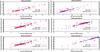 |
Fig. 2 Results of the self-calibration simulation for the synthesized images
|


3.4. Results
To be able to have a large number of realizations, we run the simulation for an array of nine primary horns, nine bolometers, and ten pointings for 100 realizations. Figure 2 shows the result of the self-calibration simulation. The six plots are scatter plots of ideal vs. real synthesized images in red and of recovered vs. real synthesized images in blue for the X and Y focal planes and each Stokes parameter I, Q, and U. The synthesized images are computed with Eq. (31), the ideal synthesized images are the synthesized images without systematic effects, the real synthesized images are the simulated measurements, and the recovered synthesized images are computed with the output parameters of the self-calibration simulation. The six plots show the advantage of the self-calibration method.
This method allows access to the systematic effects of the horns and of the half-wave
plate. It also allows calibrating the parameters and
 that completely characterize the instrument for each channel of pointings, horns, and
bolometers.
that completely characterize the instrument for each channel of pointings, horns, and
bolometers.
In running the simulation, one can find that the residual error on each output parameter will depend on the number of horns, bolometers, pointings, baselines per pointings, and on the time spent measuring each baseline. Adding more horns, pointings, bolometers, and baselines increases the mathematical constraints on a given measurement, it allows to form new baselines and adds redundancy on the horn array. Figure 3 shows that the residual diagonal term error of the Jones matrix of the half-wave plate improves as the number of baselines per pointing is higher. This result was obtained for a simulation with nine primary horns, nine bolometers and ten pointings for 40 realizations and for a time spent on each baseline tb = 1 s. The baselines measured for each pointing are chosen randomly. Similar plots are obtained with the other parameters defined in Table 2.
One can put together these variables and define a power law that allows calculating the
residual error on each parameter defined in Table 1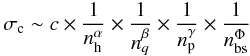 (40)with
c a constant and α, β,
γ, Φ the exponent of the number of
horns nh, bolometers nq,
pointings np, and the percent of baselines per pointing
nbs.
(40)with
c a constant and α, β,
γ, Φ the exponent of the number of
horns nh, bolometers nq,
pointings np, and the percent of baselines per pointing
nbs.
The values for each index are summarized in Table 2 for two different measuring times per baseline tb = 1 and tb = 100 s.
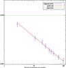 |
Fig. 3 Results of the self-calibration simulation for the diagonal terms of the Jones
matrix of the half-wave plate and a time spent per
baseline tb = 1 s. This plot represents the residual
error on these parameters as a function of the percent of baselines per pointing.
The red line represents a power law of the shape
|

One can observe in Table 2 that the error on the different reconstructed parameters is better when the time spent on each baseline is longer. Figure 4 represents the residual half-wave plate gain error as a function of the time spent on each baseline during the calibration mode. It shows that the limitation of the accuracy achieved on the systematic parameters is given by the time spent on calibration mode for each baseline tb.
The first QUBIC module will contain 400 primary horns, or 79800 baselines; therefore, we need to spend about 22h on calibration in order to measure all the baselines during one second. This lapse of time could, however, be much reduced with a small information loss if the self-calibration procedure was not performed on all baselines. The accuracy on the output parameters also depends on the number of baselines per measurement as illustrated in Fig. 3. It will be important to determine which is the most interesting strategy for the QUBIC instrument.
Using the law given by Eq. (40), one can extrapolate the result given in Table 2 to the residual error for the QUBIC instrument with 400 horns, 2 × 1024 bolometers, and 1000 pointings for two different measuring times per baseline tb = 1 and tb = 100 s. The result is given in Table 3. The values of the standard deviation between the corrupted and reconstructed parameters are obtained by replacing in Eq. (40) the values of exponent given in Table 2 applied to the design of the QUBIC instrument. It shows a very significant improvement on the level of the residual systematics after self-calibration, even for 1 s.
Results of the self-calibration simulation for an instrument with 9 horns, 9 bolometers, and 10 pointings.
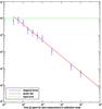 |
Fig. 4 Results of the self-calibration simulation for the diagonal terms of the Jones
matrix of the half-wave plate. We show the residual error (in blue) on these
parameters as a function of the measuring time spent on each baseline on the
calibration mode. The red line represents a power law of the shape
|

3.5. Finding limits
Accordingly Eq. (34), in an ideal case,
in the absence of systematic effects, the powers measured on the x and
y polarized focal planes after demodulation of the half-wave plate are
![Mathematical equation: \begin{eqnarray} \left ( \begin{array}{c} T_{\rm O}^\eta \\[1mm] T_{\rm C}^\eta \\[1mm] T_{\rm S}^\eta \end{array} \right ) &=& \left ( \begin{array}{c} S_I^\eta \\[1mm] S_Q^\eta \\[1mm] S_U^\eta \end{array} \right ) = \int \left ( \begin{array}{c c c} B^\eta_{q,s}(\hat{n}_{\rm p})& 0& 0\\[1mm] 0 & \epsilon^\eta B^\eta_{q,s}(\hat{n}_{\rm p}) & 0\\[1mm] 0&0&\epsilon^\eta B^\eta_{q,s}(\hat{n}_{\rm p}) \end{array} \right ) \nonumber\\ &&\bullet \left ( \begin{array}{c} I(\hat{n}_{\rm p}) \\[1mm] Q(\hat{n}_{\rm p}) \\[1mm] U(\hat{n}_{\rm p}) \end{array} \right ) {\rm d}\nu {\rm d}\hat{d}_qd\hat{n}_{\rm p} \label{eq:eq43} \end{eqnarray}](/articles/aa/full_html/2013/02/aa20429-12/aa20429-12-eq198.png) (41)with
ϵx = 1 for the polarization
x, ϵy = −1 for the
polarization y, TO,
TC, and TS refer to a constant,
cosine, and sine terms obtained after the demodulation of the half-wave plate,
SI,
SQ, and
SU refer to the synthesized images for
each Stokes parameter I, Q, and U and
(41)with
ϵx = 1 for the polarization
x, ϵy = −1 for the
polarization y, TO,
TC, and TS refer to a constant,
cosine, and sine terms obtained after the demodulation of the half-wave plate,
SI,
SQ, and
SU refer to the synthesized images for
each Stokes parameter I, Q, and U and
 the synthesized beam. The
integrations are performed over the bandwidth of the instrument, over the surface of the
bolometer, and over the sky direction.
the synthesized beam. The
integrations are performed over the bandwidth of the instrument, over the surface of the
bolometer, and over the sky direction.
For a real instrument, in the case where the half-wave plate is located before the horns,
leakages from Q to U and from U
to Q appear. Using the self-calibration simulation, one can estimate
the leakage from Q into U and from U
into Q by calculating the standard deviation of the difference between
the ideal and corrupted parameters  ,
,
 ,
,
 ,
,
 , and
, and
 (without
self-calibration) and of the difference between the corrupted and recovered parameters
(without
self-calibration) and of the difference between the corrupted and recovered parameters
 ,
,
 ,
,
 , and
, and
 (with
self-calibration).
(with
self-calibration).
In the case without self-calibration, Eq. (41) becomes ![Mathematical equation: \begin{equation} \begin{pmatrix} \Delta T_{\rm O} \\[1.5mm] \Delta T_{\rm C} \\[1.5mm] \Delta T_{\rm S} \end{pmatrix}= \begin{pmatrix} \sigma^{I}_{{\rm id}-{\rm corr}}& 0& 0\\[1.5mm] 0 &\sigma^{Q}_{{\rm id}-{\rm corr}} & \sigma^{UQ}_{{\rm id}-{\rm corr}}\\[1.5mm] 0&\sigma^{QU}_{{\rm id}-{\rm corr}}&\sigma^{U}_{{\rm id}-{\rm corr}} \end{pmatrix} \bullet \begin{pmatrix} I(\hat{n}_{\rm p}) \\[1.5mm] Q(\hat{n}_{\rm p}) \\[1.5mm] U(\hat{n}_{\rm p}) \end{pmatrix} \label{eq:eq44}. \end{equation}](/articles/aa/full_html/2013/02/aa20429-12/aa20429-12-eq215.png) (42)In the case with
self-calibration, Eq. (41) becomes
(42)In the case with
self-calibration, Eq. (41) becomes
![Mathematical equation: \begin{equation} \begin{pmatrix} \Delta T_{\rm O} \\[1.5mm] \Delta T_{\rm C} \\[1.5mm] \Delta T_{\rm S} \end{pmatrix}= \begin{pmatrix} \sigma^{I}_{{\rm corr}-{\rm rec}}& 0& 0\\[1.5mm] 0 &\sigma^{Q}_{{\rm corr}-{\rm rec}} & \sigma^{UQ}_{{\rm corr}-{\rm rec}}\\[1.5mm] 0&\sigma^{QU}_{{\rm corr}-{\rm rec}}&\sigma^{U}_{{\rm corr}-{\rm rec}} \end{pmatrix} \bullet \begin{pmatrix} I(\hat{n}_{\rm p}) \\[1.5mm] Q(\hat{n}_{\rm p}) \\[1.5mm] U(\hat{n}_{\rm p}) \end{pmatrix}. \label{eq:eq45} \end{equation}](/articles/aa/full_html/2013/02/aa20429-12/aa20429-12-eq216.png) (43)With Eqs. (42) and (43), one can observe that instrument errors and systematic effects
induce leakage from Q to U and from U
to Q but also alter the polarization amplitude. It is assumed that
there is no correlation of the errors in the synthesized beam
across the bolometers, and the
simulation is realized for a point source so that the sky convolution can be ignored.
(43)With Eqs. (42) and (43), one can observe that instrument errors and systematic effects
induce leakage from Q to U and from U
to Q but also alter the polarization amplitude. It is assumed that
there is no correlation of the errors in the synthesized beam
across the bolometers, and the
simulation is realized for a point source so that the sky convolution can be ignored.
Results of the self-calibration simulation for the QUBIC instrument with 400 horns, 2 × 1024 bolometers array, 1000 pointings, and all baseline measurements.
It is interesting to focus on the B-mode power spectrum in order to estimate the E-B
mixing and to constrain the E-mode leakage in the B-mode power spectrum. In general, one
can define the vector  that defines the errors on Stokes parameters
 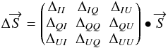 (44)where
 , and
, and
 is the vector of
measured Stokes parameters and
is the vector of
measured Stokes parameters and  is the vector of the
Stokes parameters obtained with the self-calibration method. For the QUBIC instrument,
there is no leakage of I to Q and U
because the half-wave plate is in front of the instrument so, Eq. (44) becomes
is the vector of the
Stokes parameters obtained with the self-calibration method. For the QUBIC instrument,
there is no leakage of I to Q and U
because the half-wave plate is in front of the instrument so, Eq. (44) becomes 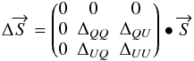 (45)where
ΔQQ, ΔQU,
ΔUQ, and ΔUU are the errors
between the synthesized beam without the self-calibration method and the one after
applying the self-calibration method. Following Appendix B and Eq. (45), one can write the error terms as
ΔQQ = 1 + ϵ,
ΔQU = ρ,
ΔUQ = −ρ, and
ΔUU = 1 + ϵ where the complex term
ϵ changes the amplitude of polarization and ρ mixes
both the Q and U Stokes parameters. One can define the
error matrix on the Q and U Stokes parameters as
Ms − 11 where the matrix
Ms is given by
(45)where
ΔQQ, ΔQU,
ΔUQ, and ΔUU are the errors
between the synthesized beam without the self-calibration method and the one after
applying the self-calibration method. Following Appendix B and Eq. (45), one can write the error terms as
ΔQQ = 1 + ϵ,
ΔQU = ρ,
ΔUQ = −ρ, and
ΔUU = 1 + ϵ where the complex term
ϵ changes the amplitude of polarization and ρ mixes
both the Q and U Stokes parameters. One can define the
error matrix on the Q and U Stokes parameters as
Ms − 11 where the matrix
Ms is given by
 (46)To go further, one can
estimate the leakage from E to B-mode and give a constraint on the value of the
tensor-to-scalar ratio r. An error in diagonal terms
ΔQQ and ΔUU will affect the
amplitude of the E and B-mode power spectrum. The nondiagonal terms
ΔQU and ΔUQ result in a
leakage from the E to B-mode power spectrum (or the B to E-mode power spectrum). To have a
constraint on the B-mode, as the E-mode is far above that of the B-mode in amplitude, one
can use the equation derived by (Rosset et al. 2010) obtained with the first-order approximation
(46)To go further, one can
estimate the leakage from E to B-mode and give a constraint on the value of the
tensor-to-scalar ratio r. An error in diagonal terms
ΔQQ and ΔUU will affect the
amplitude of the E and B-mode power spectrum. The nondiagonal terms
ΔQU and ΔUQ result in a
leakage from the E to B-mode power spectrum (or the B to E-mode power spectrum). To have a
constraint on the B-mode, as the E-mode is far above that of the B-mode in amplitude, one
can use the equation derived by (Rosset et al. 2010) obtained with the first-order approximation  (47)where
ΔClBB is the error on the B-mode power
spectrum ClBB and
ClEE is the E-mode power spectrum, and we
suppose ϵ is small. One can refer to Appendix B for the explicit
details of this equation. It shows that the uncertainty on parameter ρ
must be lower than 0.5% to have a leakage from E to B-mode lower than 10% of the expected
B-mode power spectrum ClBB for a
tensor-to-scalar ratio of r = 0.01 for
l < 100.
(47)where
ΔClBB is the error on the B-mode power
spectrum ClBB and
ClEE is the E-mode power spectrum, and we
suppose ϵ is small. One can refer to Appendix B for the explicit
details of this equation. It shows that the uncertainty on parameter ρ
must be lower than 0.5% to have a leakage from E to B-mode lower than 10% of the expected
B-mode power spectrum ClBB for a
tensor-to-scalar ratio of r = 0.01 for
l < 100.
From Eq. (47), one can estimate the leakage from the E-mode into the B-mode power spectrum given by the term ρ2ClEE. Figure 5 represents the error on the B-mode power spectrum ΔCl as a function of the multipoles. The leakage from the E-mode into the B-mode is therefore significantly reduced by applying the self-calibration procedure, even with a modest 1s per baseline (corresponding to a full day dedicated to self-calibration). The leakage can be further reduced by spending more time on self-calibration.
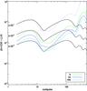 |
Fig. 5 ΔCl due to leakage from E-mode for different times on measurements per baseline tb = 1 s, 10 s and, 100 s for the QUBIC instrument. The colored solid lines represent the leakage after applying the self-calibration method for different measuring times per baseline. The dashed line represents the error on the B-mode power spectrum without self-calibration method. The black lines are the primordial B-mode spectrums for r = 10-1, r = 10-2, and r = 10-3. |
4. Conclusion
Bolometric interferometry differs considerably from standard radio interferometry in the sense that its primary goal is not to reach a good angular resolution but to achieve high statistical sensitivity and good control of systematic effects. In this perspective, redundancy turns out to be the crucial property to fulfill these two objectives, as shown in Charlassier et al. (2009) and in the present article.
In this paper, we have shown that with a polarized calibration source and the use of the successive observation of this source with all pairs of horns of the interferometer (self-calibration), one can have low and controllable instrumental systematic effects. Redundant baselines should give the same signal if they are free of systematics. By modeling the instrument systematics with a set of parameters (Jones matrices, location of the horns, beams), one can use the measurements of the different baselines to solve a nonlinear system that allows the systematic effects parameters to be determined with an accuracy that, besides the correctness of the modelling, is only limited by the photon noise, hence by the time spent on self-calibration. The more horns and bolometers in the array, the more efficient the self-calibration procedure.
The resolution of the system is CPU-intensive for large bolometric interferometers and should be implemented on massively parallel computers in the future. Using simulations with various horns and bolometer arrays of moderate sizes, we have obtained a scaling law that allows us to extrapolate the accuracy of self-calibration to the QUBIC instrument with 400 horns, 2 × 1024 bolometer arrays and 1000 pointing directions towards the calibration source. We find that with a few seconds per baseline (corresponding to a few days spent on self-calibration), knowledge of the instrumental systematic effects parameters can be improved by at least two orders of magnitude, allowing minimization of the leakage from E into B polarization down to a tolerable level. This can be improved by spending more time on self-calibration.
The idea of developing bolometric interferometry was motivated by bringing together the imager exquisite sensitivity allowed by bolometer arrays and the ability to handle instrumental systematic effects allowed by interferometers. Bolometric interferometers have been shown to have a sensitivity similar to that of imagers (Hamilton 2008; QUBIC collaboration 2010), while we have shown in the present article that the self calibration allows achieving an excellent handling of systematic effects that has no equivalent with an imager.
If A and B are 2 × 2 matrices
defined as and , the matrix direct product of A and
B is 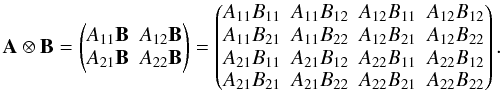
The expressions written here are only valid in the quasi-normal incidence regime. This
is not an issue, because in the next section we see that we reconstruct the actual value
of  regardless of
its exact expression.
regardless of
its exact expression.
In the case of the QUBIC instrument, the wavelength is within an order of magnitude of the detector size, consequently the field rather than the flux is being integrated over the bolometer area to take the acceptance diffraction-limited beam into account.
Acknowledgments
The authors are grateful to the QUBIC collaboration and Craig Markwardt for MPFIT. They would like to thank Gael Roudier for his help and the referee for an attentive reading. This work was supported by Agence Nationale de la Recherche (ANR), Centre National de la Recherche Scientifique (CNRS), and la région d’Ile de France.
References
- Bock, J., Church, S., Devlin, M., et al. 2006 [arXiv:astro-ph/0604101] [Google Scholar]
- Bunn, E. F. 2007, Phys. Rev. D, 75, 083517 [Google Scholar]
- Charlassier R. 2010, Ph.D., University Paris-Diderot [Google Scholar]
- Charlassier, R., Hamilton, J., Bréelle, E., et al. 2009, A&A, 497, 963 [NASA ADS] [CrossRef] [EDP Sciences] [Google Scholar]
- Charlassier, R., Bunn, E. F., Hamilton, J., Kaplan, J., & Malu, S. 2010, A&A, 514, A37 [NASA ADS] [CrossRef] [EDP Sciences] [Google Scholar]
- Hamilton, J. -C., Charlassier, R., Cressiot, C., et al. 2008, A&A, 491, 923 [NASA ADS] [CrossRef] [EDP Sciences] [Google Scholar]
- Hu, W., Hedman, M. M., & Zaldarriaga, M. 2003, Phys. Rev. D, 67, 043004 [NASA ADS] [CrossRef] [Google Scholar]
- Hyland, P., Follin, B., & Bunn, E. F. 2009, MNRAS, 393, 53 [NASA ADS] [CrossRef] [Google Scholar]
- Kovac, J., Leitch, E. M., Pryke, C., et al. 2002, Nature, 420, 772 [NASA ADS] [CrossRef] [PubMed] [Google Scholar]
- Liu, A., Tegmark, M., Morrison, S., Lutomirski, A., & Zaldarriaga, M. 2010, MNRAS, 408, 1029 [NASA ADS] [CrossRef] [Google Scholar]
- Markwardt, C. B. 2009, in ASP Conf. Ser. 411, eds. D. A. Bohlender, D. Durand, & P. Dowler, 251 [Google Scholar]
- Noordam, J. E., & de Bruyn, A. G. 1982, Nature, 299, 597 [NASA ADS] [CrossRef] [Google Scholar]
- O’Dea, D., Challinor, A., & Johnson, B. R. 2007, MNRAS, 376, 1767 [NASA ADS] [CrossRef] [Google Scholar]
- Pearson, T. J., & Readhead, A. C. S. 1984, ARA&A, 22, 97 [NASA ADS] [CrossRef] [Google Scholar]
- Readhead, A. C. S., Myers, S. T., Pearson, T. J., et al. 2004, Science, 306, 836 [NASA ADS] [CrossRef] [PubMed] [Google Scholar]
- Rosset, C., Tristram, N., Ponthieu, N., et al. 2010, A&A, 520, A13 [NASA ADS] [CrossRef] [EDP Sciences] [Google Scholar]
- Tegmark, M., & Zaldarriaga, M. 2009, Phys. Rev. D, 79, 083530 [NASA ADS] [CrossRef] [Google Scholar]
- Tegmark, M., & Zaldarriaga, M. 2012, Phys. Rev. D, 82, 103501 [NASA ADS] [CrossRef] [Google Scholar]
- The QUBIC Collaboration 2010, Astropart. Phys., 34 [Google Scholar]
- Timbie, P. T., Tucker, G. S., Ade, P. A. R., et al. 2006, New Astron. Rev., 50, 999 [NASA ADS] [CrossRef] [Google Scholar]
- Tucker, G. S., Kim, J., Timbie, P., et al. 2003, New Astron. Rev., 47, 1173 [NASA ADS] [CrossRef] [Google Scholar]
- Wieringa, M. 1991, in IAU Colloq. 131: Radio Interferometry. Theory, Techniques, and Applications, eds. T. J. Cornwell, & R. A. Perley, ASP Conf. Ser., 19, 192196 [Google Scholar]
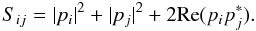
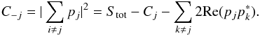
Appendix A: Measuring the bolometer power for two opened horns is equivalent to measuring the bolometer power when all horns are open except the horn i and j
The power collected by the bolometer q for the opened
horns i and j without polarization is
 (A.1)which can be written as
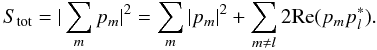
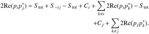
 (A.2)The total power measured
for all the baselines can be expressed as
(A.2)The total power measured
for all the baselines can be expressed as
 (A.3)The power measured by a
bolometer q for all horns opened except the horn i is
(A.3)The power measured by a
bolometer q for all horns opened except the horn i is
 (A.4)The power measured by a
bolometer q for all horns opened except the horn j is
(A.4)The power measured by a
bolometer q for all horns opened except the horn j is
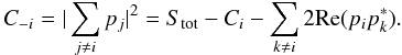
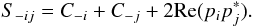
 (A.5)The power measured by a
bolometer q for all baselines opened, except the baseline formed by the horns
i and j, is
(A.5)The power measured by a
bolometer q for all baselines opened, except the baseline formed by the horns
i and j, is
 (A.6)with
 Finally,
one can find
Finally,
one can find  (A.7)So:
 (A.8)
(A.8)
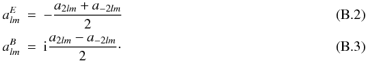
Appendix B: Error on E and B-mode power spectra
One can define the Stokes parameters in spin-2 spherical harmonics base
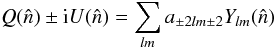 (B.1)where Q
and U are defined at each
direction
(B.1)where Q
and U are defined at each
direction  .
.
It is convenient to introduce the linear combinations
 One
can define the two scalar fields
One
can define the two scalar fields  Using
the coefficients
Using
the coefficients  and
and
 , one can
construct the angular power spectrum
, one can
construct the angular power spectrum  and
and
 as
as
 One
can express the Q and U Stokes parameters as a function
of the coefficients
and
One
can express the Q and U Stokes parameters as a function
of the coefficients
and ![Mathematical equation: \appendix \setcounter{section}{2} \begin{eqnarray} Q(\hat{n}) &= &\frac{1}{2} \sum_{l,m}\Bigg [\Bigg ({\rm i}a^{\rm B}_{lm}-a^{\rm E}_{lm} \Bigg )_{-2}Y_{lm}(\hat{n})+ \Bigg (-{\rm i}a^{\rm B}_{lm}-a^{\rm E}_{lm} \Bigg )_{+2}Y_{lm}(\hat{n}) \Bigg ] \nonumber \\ \\ U(\hat{n})& = &\frac{1}{2}\sum_{l,m}\Bigg [{\rm i} \Bigg ({\rm i} a^{\rm B}_{lm}-a^{\rm E}_{lm} \Bigg )_{-2}Y_{lm}(\hat{n})+\Bigg (-{\rm i}a^{\rm B}_{lm}-a^{\rm E}_{lm} \Bigg )_{+2}Y_{lm}(\hat{n}) \Bigg ]. \nonumber \\ \end{eqnarray}](/articles/aa/full_html/2013/02/aa20429-12/aa20429-12-eq287.png) Using
Eqs. (B.4), (B.5), (B.8), and (B.9), one can express the
coefficients
Using
Eqs. (B.4), (B.5), (B.8), and (B.9), one can express the
coefficients  and
and  as a function
of the Stokes parameters Q
and U
as a function
of the Stokes parameters Q
and U (B.10)where the
integration is taken over the whole sky, and
(B.10)where the
integration is taken over the whole sky, and
 (B.11)In the case of a
bolometric interferometer, globar errors on synthesized beam will affect the amplitude of
polarization and mix the Q and U Stokes parameters.
(B.11)In the case of a
bolometric interferometer, globar errors on synthesized beam will affect the amplitude of
polarization and mix the Q and U Stokes parameters.
To model systematic errors, one can introduce a Jones matrix that describes the
propagation of radiation through a receiver
![Mathematical equation: \appendix \setcounter{section}{2} \begin{equation} \overrightarrow{E_r}=\mathbf{J}\overrightarrow{E}= \begin{pmatrix} 1-g_{x} & e_{x} \\[1mm] e_{y} & 1-g_{y} \end{pmatrix} \overrightarrow{E} \end{equation}](/articles/aa/full_html/2013/02/aa20429-12/aa20429-12-eq292.png) (B.12)where
the gain gη and the leakage
eη are complex values.
(B.12)where
the gain gη and the leakage
eη are complex values.
From this relation, one can construct the Mueller matrix M,
which tells us how the Stokes vector
transforms 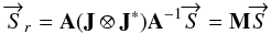 (B.13)
![Mathematical equation: \begin{equation*} \textrm{where}~ \mathbf{A}= \begin{bmatrix} 1 & 0 & 0 & 1\\[1.2mm] 1 & 0 & 0 & -1 \\[1.2mm] 0 & 1 & 1 & 0\\[1.2mm] 0 & i & -i & 0\\[1.2mm] \end{bmatrix} \end{equation*}](/articles/aa/full_html/2013/02/aa20429-12/aa20429-12-eq297.png) and
is the outgoing Stokes
vector and
M = A(J ⊗ J ∗ )A-1
is the resulting error matrix.
and
is the outgoing Stokes
vector and
M = A(J ⊗ J ∗ )A-1
is the resulting error matrix.
We are only interested in the Q and U Stokes
parameters. In this case, the error matrix M becomes
![Mathematical equation: \appendix \setcounter{section}{2} \begin{equation} \mathbf{M} = \begin{pmatrix} M_{QQ} & M_{QU} \\[1mm] M_{UQ} & M_{UU} \end{pmatrix}. \end{equation}](/articles/aa/full_html/2013/02/aa20429-12/aa20429-12-eq299.png) (B.14)The first order of this
matrix M is
(B.14)The first order of this
matrix M is ![Mathematical equation: \appendix \setcounter{section}{2} \begin{eqnarray*} M_{QQ}&=&1+g_x+g_y+g_x^*+g_y^* \\[1.2mm] M_{UQ}&=&e_y+e_y^*-e_x-e_x^* \\[1.2mm] M_{QU}&=&e_x+e_x^*-e_y-e_y^* \\[1.2mm] M_{UU}&=&1+g_x+g_y+g_x^*+g_y^*. \end{eqnarray*}](/articles/aa/full_html/2013/02/aa20429-12/aa20429-12-eq300.png) One
can generalize this error matrix for Jones matrix of any component and rewrite it as
Ms − 11 where
One
can generalize this error matrix for Jones matrix of any component and rewrite it as
Ms − 11 where
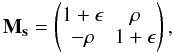 (B.15)where the complex
term ϵ describes the error of the amplitude of polarization and the
complex term ρ mixes the Q and U Stokes
parameters.
(B.15)where the complex
term ϵ describes the error of the amplitude of polarization and the
complex term ρ mixes the Q and U Stokes
parameters.
In this case, Eq. (B.10) becomes
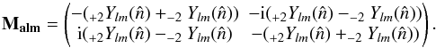
![Mathematical equation: \appendix \setcounter{section}{2} \begin{equation} \begin{pmatrix} a^{{\rm E},{\rm meas}}_{lm} \\[1.5mm] a^{{\rm B},{\rm meas}}_{lm} \end{pmatrix} = \mathbf{M_{\rm alm}}\mathbf{M_s} \begin{pmatrix} Q(\hat{n}) \\[1.5mm] U(\hat{n}) \end{pmatrix} \end{equation}](/articles/aa/full_html/2013/02/aa20429-12/aa20429-12-eq302.png) (B.16)where
the coefficients
(B.16)where
the coefficients  and
and  include systematic effects.
In terms of power spectra, an error in polarization amplitude will affect the amplitude of the E and B-mode power spectra,
and an error that mixes the Q and U Stokes parameters leads to a leakage from the E to B-mode (and from the B to E-mode).
One can easily find that with systematic effects, the coefficients
and can be
expressed as 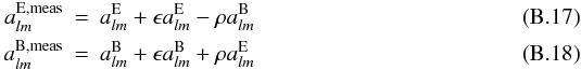 where
ϵ is the error in amplitude and ρ the error of
polarization leakage. Using Eqs. (B.6) and (B.7), one can obtain
where
ϵ is the error in amplitude and ρ the error of
polarization leakage. Using Eqs. (B.6) and (B.7), one can obtain
 (B.19)
 (B.20)where we suppose
ϵ is small,
ClEE,meas and
ClBB,meas are the E and
B-mode power spectra including systematic effects,
ClEE and
ClBB the input power spectra, the complex
term ϵ describes the error of amplitude of the B-mode power spectrum,
and the complex term ρ results in a leakage from the E to B-mode power
spectrum.
(B.20)where we suppose
ϵ is small,
ClEE,meas and
ClBB,meas are the E and
B-mode power spectra including systematic effects,
ClEE and
ClBB the input power spectra, the complex
term ϵ describes the error of amplitude of the B-mode power spectrum,
and the complex term ρ results in a leakage from the E to B-mode power
spectrum.
To focus on the B-mode, one can define the error on
ClBB power spectrum
 (B.21)
All Tables
Results of the self-calibration simulation for an instrument with 9 horns, 9 bolometers, and 10 pointings.
Results of the self-calibration simulation for the QUBIC instrument with 400 horns, 2 × 1024 bolometers array, 1000 pointings, and all baseline measurements.
All Figures
|
Fig. 1 Design of the QUBIC instrument. |
| In the text | |
|
Fig. 2 Results of the self-calibration simulation for the synthesized images
|
| In the text | |
|
Fig. 3 Results of the self-calibration simulation for the diagonal terms of the Jones
matrix of the half-wave plate and a time spent per
baseline tb = 1 s. This plot represents the residual
error on these parameters as a function of the percent of baselines per pointing.
The red line represents a power law of the shape
|
| In the text | |
|
Fig. 4 Results of the self-calibration simulation for the diagonal terms of the Jones
matrix of the half-wave plate. We show the residual error (in blue) on these
parameters as a function of the measuring time spent on each baseline on the
calibration mode. The red line represents a power law of the shape
|
| In the text | |
|
Fig. 5 ΔCl due to leakage from E-mode for different times on measurements per baseline tb = 1 s, 10 s and, 100 s for the QUBIC instrument. The colored solid lines represent the leakage after applying the self-calibration method for different measuring times per baseline. The dashed line represents the error on the B-mode power spectrum without self-calibration method. The black lines are the primordial B-mode spectrums for r = 10-1, r = 10-2, and r = 10-3. |
| In the text | |
Current usage metrics show cumulative count of Article Views (full-text article views including HTML views, PDF and ePub downloads, according to the available data) and Abstracts Views on Vision4Press platform.
Data correspond to usage on the plateform after 2015. The current usage metrics is available 48-96 hours after online publication and is updated daily on week days.
Initial download of the metrics may take a while.