| Issue |
A&A
Volume 550, February 2013
|
|
|---|---|---|
| Article Number | A53 | |
| Number of page(s) | 16 | |
| Section | Planets and planetary systems | |
| DOI | https://doi.org/10.1051/0004-6361/201220146 | |
| Published online | 24 January 2013 | |
New analytical expressions of the Rossiter-McLaughlin effect adapted to different observation techniques ⋆
1
Centro de Astrofísica, Universidade do Porto
Rua das Estrelas
4150-762
Porto
Portugal
2
Astronomie et Systèmes Dynamiques, IMCCE-CNRS UMR 8028,
Observatoire de Paris, UPMC, 77 Av.
Denfert-Rochereau, 75014
Paris,
France
3
Department of Astronomy and Astrophysics, University of
Chicago, 5640 South Ellis
Avenue, Chicago,
IL
60637,
USA
e-mail: This email address is being protected from spambots. You need JavaScript enabled to view it.
4
Departamento de Física e Astronomia, Faculdade de Ciências,
Universidade do Porto, Rua do Campo
Alegre, 4169-007
Porto,
Portugal
Received:
31
July
2012
Accepted:
31
October
2012
Abstract
The Rossiter-McLaughlin (hereafter RM) effect is a key tool for measuring the projected spin-orbit angle between stellar spin axes and orbits of transiting planets. However, the measured radial velocity (RV) anomalies produced by this effect are not intrinsic and depend on both instrumental resolution and data reduction routines. Using inappropriate formulas to model the RM effect introduces biases, at least in the projected velocity Vsini⋆ compared to the spectroscopic value. Currently, only the iodine cell technique has been modeled, which corresponds to observations done by, e.g., the HIRES spectrograph of the Keck telescope. In this paper, we provide a simple expression of the RM effect specially designed to model observations done by the Gaussian fit of a cross-correlation function (CCF) as in the routines performed by the HARPS team. We derived a new analytical formulation of the RV anomaly associated to the iodine cell technique. For both formulas, we modeled the subplanet mean velocity vp and dispersion βp accurately taking the rotational broadening on the subplanet profile into account. We compare our formulas adapted to the CCF technique with simulated data generated with the numerical software SOAP-T and find good agreement up to Vsini⋆ ≲ 20 km s-1. In contrast, the analytical models simulating the two different observation techniques can disagree by about 10σ in Vsini⋆ for large spin-orbit misalignments. It is thus important to apply the adapted model when fitting data.
Key words: techniques: spectroscopic / instrumentation: spectrographs / planetary systems / methods: analytical / methods: data analysis
A public code implementing the expressions derived in this paper is available at http://www.astro.up.pt/resources/arome. A copy of the code is also available at the CDS via anonymous ftp to cdsarc.u-strasbg.fr (130.79.128.5) or via http://cdsarc.u-strasbg.fr/viz-bin/qcat?J/A+A/550/A53
© ESO, 2013
1. Introduction
Transiting planets produce radial velocity (RV) anomalies when crossing the disk of their star. This mechanism, known as the Rossiter-McLaughlin effect (hereafter RM effect), is due to the stellar proper rotation and the fact that during a transit, a planet successively covers different portions of the stellar disk with different average velocities along the line of sight (Holt 1893; Rossiter 1924; McLaughlin 1924). The RM effect has gained importance in the exoplanet community since it allows the measurement of the projected angle between the stellar spin-axis and the orbit of the planet.
 |
Fig. 1 Simplified illustration of different methods to compute the Rossiter-McLaughlin effect. vH10, viodine, and vCCF represent the result of the hypothesis made in Hirano et al. (2010), the result of the data reduction done with the iodine cell technique, and the result of the data reduction done with the CCF technique, respectively. |
The first measurements of the RM effect induced by a transiting planet were performed almost simultaneously with two different instruments on the same bright star HD 209458. Queloz et al. (2000) observed the signal with the ELODIE spectrograph on the 193 cm telescope of the Observatoire de Haute Provence, while Bundy & Marcy (2000) used the HIRES spectrograph on the Keck telescope. As explained later on, the choice of the instrument and, more particularly, the subsequent reduction analysis, have a non negligible impact on the resulting shape of signal. It is thus interesting to see that the two kinds of instrument, coupled with their own data treatment, which are still employed today, have been used in parallel since the beginning.
The first planet-host stars studied with this technique were all compatible with low obliquity. It was along the lines of the model of planet migration in a protoplanetary disk. But then, several misaligned systems have been detected, starting with XO-3 with an angle initially announced at 70° ± 15° (Hébrard et al. 2008) and then refined to 37.3° ± 3° (Winn et al. 2009), yet still significantly misaligned. With the growth of the sample, a first correlation appeared showing that the hottest stars tend to be more misaligned (Winn et al. 2010). Additionally, a first statistical comparison between observations and theoretical predictions have been performed (Triaud et al. 2010), suggesting that some of the hot Jupiters might be the result of the interaction with a stellar companion, leading to a Lidov-Kozai mechanism, characterized by phases of large eccentricity and inclination and followed by a circularization by tides raised on the planet as it approaches the star (Wu & Murray 2003; Fabrycky & Tremaine 2007). Other scenarios have then been developed to explain the formation of hot Jupiters, such as planet-planet scattering (Rasio & Ford 1996; Beaugé & Nesvorný 2012), the crossing of secular resonances (Wu & Lithwick 2011), or the Lidov-Kozai mechanism produced by a planetary companion (Naoz et al. 2011; Nagasawa & Ida 2011). A new trend between age and obliquity has also been found (Triaud 2011) suggesting that tidal dissipation may play an important role in the evolution of those systems, as confirmed by Albrecht et al. (2012).
Accurate modelings of the RM effect are thus needed to get reliable information on the current obliquity of stars and to test theoretical predictions. In the literature, one can find several analytical expressions to model this effect (Kopal 1942; Ohta et al. 2005; Giménez 2006; Hirano et al. 2010, 2011). They are not all identical because they model different techniques of radial velocity measurements.
This raises an issue that should be considered with caution. RVs measured by different techniques or even by different instruments using the same algorithm can differ by more than a constant offset. To illustrate this point, we consider a random variable with a given probability distribution function (PDF), and ask what its average value is. The term average is vague and can mean different quantities: mean, median, mode, etc. Nevertheless, if the PDF is symmetrical, any of these quantities lead to the same result, eventually with different robustnesses with respect to noise. But if the PDF is not symmetrical, each estimator of the average value provides different results that cannot be compared directly. The situation is similar in RV observations, as noticed by Hirano et al. (2010). There are at least two different ways to measure RVs. One relies on the iodine cell technique which consists in fitting an observed spectrum with a modeled one that is Doppler-shifted (Butler et al. 1996). The other is based on a Gaussian fit to a cross-correlation function (CCF) (Baranne et al. 1996; Pepe et al. 2002). The former technique is applied to observations made with HIRES on the Keck telescope or with HDS at the Subaru telescope, while the latter is the routine of, e.g., SOPHIE at the Observatoire de Haute Provence or HARPS at La Silla Observatory. If stars are affected by neither spots nor transiting planets, their spectral lines have constant shapes, and thus the RVs derived by any instruments may only differ by a constant offset. In contrast, spectral lines are deformed during transits, and these deformations vary with time. As a consequence, each analysis routine is expected to lead to a different signal. In turn, it is important to have an analytical model adapted to each analysis routine in order to interpret RM data. Moreover, it also means that one should not combine RM measurements from different instruments.
The first analytical expressions of the RM effect were derived by Kopal (1942), Ohta et al. (2005),
and Giménez (2006). They all computed the weighted
mean velocity, hereafter called vmean, along the line of sight
of the stellar surface uncovered by the planet. This mean velocity, weighted by the surface
intensity, leads to an exact expression of the form  (1)where
f is the fraction of the flux blocked by the planet disk
and vp is the average velocity of the surface of the star
covered by the planet. This expression is simple and exact. There is no assumption behind
it. But, it does not correspond to the quantity that is actually measured in the
observations by either the iodine cell technique, or by the Gaussian fit of the CCF. Thus,
the analytical prediction vmean is systematically biased when
compared directly with observations. The difference increases for high stellar rotational
velocities.
(1)where
f is the fraction of the flux blocked by the planet disk
and vp is the average velocity of the surface of the star
covered by the planet. This expression is simple and exact. There is no assumption behind
it. But, it does not correspond to the quantity that is actually measured in the
observations by either the iodine cell technique, or by the Gaussian fit of the CCF. Thus,
the analytical prediction vmean is systematically biased when
compared directly with observations. The difference increases for high stellar rotational
velocities.
To solve this problem, Hirano et al. (2010) propose
a new analytical expression closely related to the reduction algorithm of the iodine cell
technique (see Fig. 1). This method consists in fitting
a shifted spectrum outside of transits, which is modeled, here, by a single averaged
spectral line and noted1 ,
with the line profile detected during a transit ℱtransit(v), via
the Doppler shift
,
with the line profile detected during a transit ℱtransit(v), via
the Doppler shift  .
The quantity provided by the formulas of Hirano et al.
(2010) is the value, hereafter denoted vH10, of the
velocity
that maximizes the cross-correlation between the two line profiles
.
The quantity provided by the formulas of Hirano et al.
(2010) is the value, hereafter denoted vH10, of the
velocity
that maximizes the cross-correlation between the two line profiles
 . We show
in Sect. 3.1 that if ℱstar is an even
function, the maximization of the cross-correlation
. We show
in Sect. 3.1 that if ℱstar is an even
function, the maximization of the cross-correlation  is indeed identical to the minimization of the chi-square associated to the fit of
ℱtransit(v) by .
In that case, the result depends on the actual shape of the line profiles, as observed in
practice. In the simplest case where the line profiles of both the nonrotating and the
rotating star are Gaussian, this method leads to (Hirano
et al. 2010)
is indeed identical to the minimization of the chi-square associated to the fit of
ℱtransit(v) by .
In that case, the result depends on the actual shape of the line profiles, as observed in
practice. In the simplest case where the line profiles of both the nonrotating and the
rotating star are Gaussian, this method leads to (Hirano
et al. 2010)  (2)where
β⋆ and βp are
the dispersion of the Gaussian profiles ℱstar(v) and
ℱpla(v − vp) respectively2.
ℱpla(v − vp) is the line profile
of the light blocked by the planet centered on vp. Although this
expression is the result of an expansion in both f and
vp, it gives a better representation of the measured radial
velocity. Hirano et al. (2010) also provide more
complex expressions in the case of Voigt profiles, and in Hirano et al. (2011), additional effects are taken into account such as
macro-turbulence. But the result is not expressed as a simple analytical formula and it
requires several numerical integrations.
(2)where
β⋆ and βp are
the dispersion of the Gaussian profiles ℱstar(v) and
ℱpla(v − vp) respectively2.
ℱpla(v − vp) is the line profile
of the light blocked by the planet centered on vp. Although this
expression is the result of an expansion in both f and
vp, it gives a better representation of the measured radial
velocity. Hirano et al. (2010) also provide more
complex expressions in the case of Voigt profiles, and in Hirano et al. (2011), additional effects are taken into account such as
macro-turbulence. But the result is not expressed as a simple analytical formula and it
requires several numerical integrations.
The model of Hirano et al. (2010, 2011) is well adapted to the iodine cell technique, but it still does not correspond to the analysis routines used on stabilized spectrographs, e.g., SOPHIE and HARPS (Baranne et al. 1996; Pepe et al. 2002). In these routines, the observed spectrum is first cross-correlated with a template spectrum. This gives the so-called cross-correlation function (CCF) which can be seen as a weighted average of all the spectral lines convolved with a rectangular function. Finally, the CCF is fitted by a Gaussian whose mean represents the observed radial velocity vCCF (see Fig. 1). Currently, there is no analytical expression of this quantity in the literature. The goal of this paper is to provide such an expression. As we will see, even in the general case where the spectral line profile ℱstar is not Gaussian, the resulting formula is as simple as Eq. (2) derived by Hirano et al. (2010) and exact in vp.
This paper is organized as follows. In Sect. 2, we analytically derive an unbiased expression vCCF modeling the RM effect as measured by, e.g., SOPHIE and HARPS. This formula is specially designed to simulate the radial velocity measurements obtained by fitting a Gaussian to a CCF. We first provide very generic expressions that relies only on the symmetry of the spectroscopic lines, and then, we give a much simpler formula corresponding to Gaussian subplanet line profiles. In Sect. 3, we propose a new expression viodine of the RM signal derived by the iodine technique. In comparison to the previous ones, it is analytical and valid for any spectroscopic Vsini⋆. Then, in Sect. 4, we detail the calculation of the parameters entering into our formulas vCCF and viodine, which are the flux fraction f occulted by the planet, the subplanet velocity vp, and the dispersion βp. In Sect. 5, we compare our analytical results with simulated data generated with SOAP-T, a modified version of the numerical code SOAP (Boisse et al. 2012), able to reproduce RM signals (Oshagh et al. 2013). We also analyze biases introduced by the application of a wrong model in the fit of RM signals. Finally, we conclude in Sect. 6.
2. Modeling of the RM effect measured by the CCF technique
2.1. General derivation
We derive a very general expression of the RM effect obtained using a Gaussian fit to the
CCF. As in Hirano et al. (2010), we only consider
the linear effect with respect to the flux ratio f. But the method can
easily be generalized to higher orders. We define ℱstar(v),
ℱpla(v − vp), and
ℱtransit(v) the line profile of the CCF produced by the
integrated stellar surface, by the part of the stellar surface covered by the planet, and
by the uncovered stellar surface, respectively. At this stage, the line profiles
ℱstar, ℱpla, and ℱtransit are not necessarily Gaussian.
The dependency of ℱpla is on
(v − vp) because this line is centered on
vp. By convention, ℱstar(v) and
ℱpla(v − vp) are normalized to
one. With this convention, even absorption spectral lines are positive.
We have
ℱtransit(v) = ℱstar(v) − fℱpla(v − vp).
Moreover, we denote  as the unit Gaussian profile with dispersion σ and centered on the origin
 (3)The fit of the CCF
measured during transit, ℱtransit(v), by a Gaussian
corresponds to the maximization of the likelihood
(3)The fit of the CCF
measured during transit, ℱtransit(v), by a Gaussian
corresponds to the maximization of the likelihood
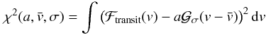 (4)with respect to the
normalization factor a, the mean velocity
,
and the dispersion σ. The partial derivatives read as
(4)with respect to the
normalization factor a, the mean velocity
,
and the dispersion σ. The partial derivatives read as 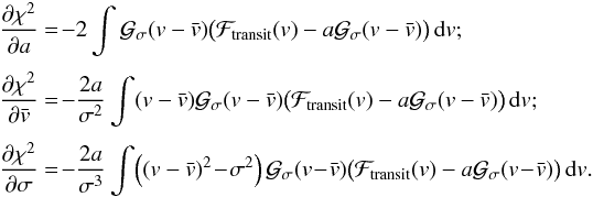 (5)We
now set all the derivatives to zero, express ℱtransit(v) as a
function of ℱstar(v) and ℱpla(v),
and reorder the terms. The system of Eqs. (5) is equivalent to
(5)We
now set all the derivatives to zero, express ℱtransit(v) as a
function of ℱstar(v) and ℱpla(v),
and reorder the terms. The system of Eqs. (5) is equivalent to 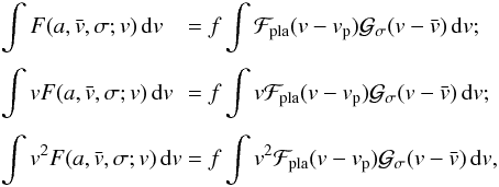 (6)with
 (7)To solve this system, we
apply the usual perturbation method. We develop the parameters in series of the flux ratio
f, i.e.,
a = a0 + fa1 + f2a2 + ...,
and idem for
and σ. At the zeroth order in f, the system (6) corresponds to the fit of
ℱstar(v) by a Gaussian. The effect of the planet is absent
from the fit, thus
(7)To solve this system, we
apply the usual perturbation method. We develop the parameters in series of the flux ratio
f, i.e.,
a = a0 + fa1 + f2a2 + ...,
and idem for
and σ. At the zeroth order in f, the system (6) corresponds to the fit of
ℱstar(v) by a Gaussian. The effect of the planet is absent
from the fit, thus  .
The other parameters a0 and σ0 are
those of the best Gaussian fit outside of transits.
.
The other parameters a0 and σ0 are
those of the best Gaussian fit outside of transits.
In a second step, we linearize the system (6) in the vicinity of the zeroth order solution. We thus compute the partial
derivatives of 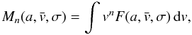 (8)appearing in the
left-hand side of (6), at
a = a0,
(8)appearing in the
left-hand side of (6), at
a = a0,
 ,
and σ = σ0. To avoid fastidious calculation,
we make the simple hypothesis that ℱstar(v) is symmetrical, or
more precisely, an even function of the velocity v. In practice, due to
the convective blue shift (CB), spectral lines are not perfectly symmetric. The net effect
of CB is a small deformation in RM signals with amplitude of order 1 m s-1
(Albrecht et al. 2012) that we neglect. Then,
,
and σ = σ0. To avoid fastidious calculation,
we make the simple hypothesis that ℱstar(v) is symmetrical, or
more precisely, an even function of the velocity v. In practice, due to
the convective blue shift (CB), spectral lines are not perfectly symmetric. The net effect
of CB is a small deformation in RM signals with amplitude of order 1 m s-1
(Albrecht et al. 2012) that we neglect. Then,
 and
and  are even functions of ,
while
are even functions of ,
while  is odd. As a result, the derivatives
  ,
,
 ,
∂M1/∂a,
and
∂M1/∂σ
taken at
,
∂M1/∂a,
and
∂M1/∂σ
taken at  vanish. Moreover, if the subplanet line profile is also an even function then the
integrals of the righthand side of the system (6) become simple convolutions at .
Then there is only
vanish. Moreover, if the subplanet line profile is also an even function then the
integrals of the righthand side of the system (6) become simple convolutions at .
Then there is only  ,\notag \\ \left(\Dron{M_1}{\vx}\right) \vx_1& &= \left[(v\,\Gfitb)*\Fpla\right](v_{\rm p}) ,\notag \\ \left(\Dron{M_2}{a}\right) a_1& +\left(\Dron{M_2}{\sigma}\right) \sigma_1 &= \left[(v^2\Gfitb)*\Fpla\right](v_{\rm p}) , \end{eqnarray}](/articles/aa/full_html/2013/02/aa20146-12/aa20146-12-eq57.png) (9)where
∗ denotes the convolution product. The first and the third lines are independent of the
mean velocity
(9)where
∗ denotes the convolution product. The first and the third lines are independent of the
mean velocity  .
Their resolution provides a correction to the amplitude and the width of the best Gaussian
fit during a transit. The second equation is the most interesting, since it contains the
quantity
we are looking for. By chance, this is also the simplest. The velocity anomaly obtained by
the Gaussian fit
.
Their resolution provides a correction to the amplitude and the width of the best Gaussian
fit during a transit. The second equation is the most interesting, since it contains the
quantity
we are looking for. By chance, this is also the simplest. The velocity anomaly obtained by
the Gaussian fit  is then
  \end{equation}](/articles/aa/full_html/2013/02/aa20146-12/aa20146-12-eq61.png) (10)where
(10)where
 should be computed at
(a0,0,σ0),
i.e.,
should be computed at
(a0,0,σ0),
i.e.,  . \label{eq.dM1dv} \end{eqnarray}](/articles/aa/full_html/2013/02/aa20146-12/aa20146-12-eq64.png) (11)The
convolution product taken at 0 on the righthand side of (11) is nothing else but M2, which cancels
by the definitions of a0 and σ0.
Thus the RM effect now reads as
(11)The
convolution product taken at 0 on the righthand side of (11) is nothing else but M2, which cancels
by the definitions of a0 and σ0.
Thus the RM effect now reads as ![Mathematical equation: \begin{equation} \vc = -\frac{4\sigma_0\sqrt{\pi}}{a_0} f \left[\left(v\,\Gfitb\right)*\Fpla)\right]\left(v_{\rm p}\right). \label{eq.solgen} \end{equation}](/articles/aa/full_html/2013/02/aa20146-12/aa20146-12-eq66.png) (12)This expression does
not depend directly on the stellar line profile ℱstar. The dependence only
occurs through the best Gaussian fit (a0 and
σ0), which is performed to derive the radial velocity. The
formula (12) is thus very powerful, since
it does not require any knowledge on ℱstar. Unfortunately, the
amplitude a0 of the best Gaussian fit in (12) is associated to a normalized line
profile ℱstar while, in practice, the area of a CCF is difficult to measure,
and ℱstar is never normalized. We thus provide the expression of
a0 as a function of ℱstar and the best Gaussian
fit
(12)This expression does
not depend directly on the stellar line profile ℱstar. The dependence only
occurs through the best Gaussian fit (a0 and
σ0), which is performed to derive the radial velocity. The
formula (12) is thus very powerful, since
it does not require any knowledge on ℱstar. Unfortunately, the
amplitude a0 of the best Gaussian fit in (12) is associated to a normalized line
profile ℱstar while, in practice, the area of a CCF is difficult to measure,
and ℱstar is never normalized. We thus provide the expression of
a0 as a function of ℱstar and the best Gaussian
fit  ,
,
 . \label{eq.a0} \end{equation}](/articles/aa/full_html/2013/02/aa20146-12/aa20146-12-eq68.png) (13)We emphasize that
a0 is independent of vp. As a
consequence, it does not affect the shape of the RM effect, but only slightly the
amplitude (a0 remains close to one). The computation of
a0 is detailed in Appendix B.
(13)We emphasize that
a0 is independent of vp. As a
consequence, it does not affect the shape of the RM effect, but only slightly the
amplitude (a0 remains close to one). The computation of
a0 is detailed in Appendix B.
2.2. Gaussian subplanet line profile
At this stage, the expression (12) is very general, and holds as long as the line profiles ℱstar(v) and ℱpla(v) are symmetric.
We now make the hypothesis that the subplanet line profile
ℱpla(v) is Gaussian. It should be stressed that, as long as
the planet radius is small compared to that of the star, the subplanet line profile is
only weakly affected by the stellar rotation (see Sect. 4) and thus, it is well approximated by that of the nonrotating star, which we
assume to be Gaussian. Then, the subplanet profile can be considered Gaussian, or equal to
the sum of two Gaussians if macro-turbulence is taken into account (see Appendix A). We denote βp as the
width of the subplanet line profile, i.e.,  .
In that case, the expression of the RM effect (12) becomes
.
In that case, the expression of the RM effect (12) becomes  (14)This is the main equation
of this paper. It represents a good compromise between simplicity and accuracy for the
modeling of RM signals measured by a Gaussian fit of the CCF.
(14)This is the main equation
of this paper. It represents a good compromise between simplicity and accuracy for the
modeling of RM signals measured by a Gaussian fit of the CCF.
2.3. Gaussian stellar line profile
For completeness, we give the expression in the case where the stellar line profile is a
normalized Gaussian with dispersion β⋆. The
best fit should give a0 = 1 and
σ0 = β⋆.
Then, we get 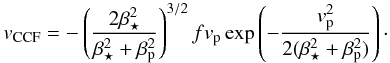 (15)This formula is
equivalent to vH10 (2) given by Hirano et al. (2010). More
precisely, Eq. (2) is the beginning of the
expansion of vCCF. Indeed, if the stellar line profile is
Gaussian, the two approaches are identical.
(15)This formula is
equivalent to vH10 (2) given by Hirano et al. (2010). More
precisely, Eq. (2) is the beginning of the
expansion of vCCF. Indeed, if the stellar line profile is
Gaussian, the two approaches are identical.
3. Modeling of the RM effect measured by the iodine cell technique
In this section, we first explain the equivalence between the iodine cell technique and the
maximization of the cross-correlation
(Hirano et al. 2010, 2011). The aim is to emphasize the hypotheses behind this equivalence
and, thus, to show its limitations. In a second step, we provide a general expression that
models the iodine cell technique. It should be stressed that the function
is different from the CCF of the previous section and is not used in the same way. It
involves the spectrum during transit and a modeled one without transit deformations. This
function
is computed to provide the RV at its maximum. On the other hand, the CCF is the
cross-correlation between the spectrum and a mask. The goal is to provide a single averaged
line that is then fitted by a Gaussian curve.
3.1. Link between the iodine cell technique and the maximization of
C( )
)
The analysis routine based on the iodine cell technique involves a fit with 13 parameters
of the observed spectrum by a modeled one that is Doppler-shifted (Butler et al. 1996). We assume that this can be approximated by the fit
of a single parameter ()
representing the Doppler shift between a modeled line profile
ℱstar(v) and the observed one (here during a transit)
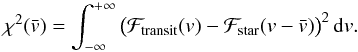
ℱtransit(v). The chi-square of this fit reads
 (16)The minimization of this
chi-square corresponds to
(16)The minimization of this
chi-square corresponds to  with
with 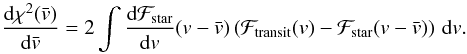 (17)The integral on the
righthand side can be split into the sum of two integrals
(17)The integral on the
righthand side can be split into the sum of two integrals
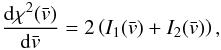 (18)where the first one,
 ,
is the cross-correlation of dℱstar/dv by
ℱtransit taken at ,
while the other is, after the change of variable
,
is the cross-correlation of dℱstar/dv by
ℱtransit taken at ,
while the other is, after the change of variable  ,
,
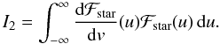 (19)If ℱstar
is even, its derivative is odd, and thus the integral I2
over R vanishes. In that case, only
(19)If ℱstar
is even, its derivative is odd, and thus the integral I2
over R vanishes. In that case, only
 (20)remains,
where ⋆ denotes the cross-correlation product defined by
(20)remains,
where ⋆ denotes the cross-correlation product defined by
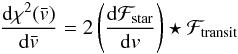
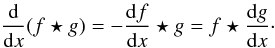
 = \int_{-\infty}^{+\infty} f(y-x)g(y)\,{\rm d}y . \end{equation}](/articles/aa/full_html/2013/02/aa20146-12/aa20146-12-eq87.png) (21)We then use the property
of the derivative of the cross-correlation of two functions
(21)We then use the property
of the derivative of the cross-correlation of two functions
 (22)By
identification, we obtain
(22)By
identification, we obtain 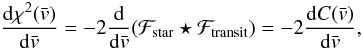 (23)where
is defined as in Hirano et al. (2010). Thus, the
minimization of the chi-square involved in the iodine cell technique is indeed equivalent
to the maximization of the cross-correlation
as computed in Hirano et al. (2010). This result
holds as long as the complicated fit with 13 parameters can be modeled by the fit of the
single parameter ,
and if the modeled line profile is symmetrical. The second condition may not be true in
general. If the asymmetry is not too strong, the integral I2
would be a small perturbation, and the result obtained by the maximization of the
cross-correlation
should differ from the minimization of the chi-square by only a small constant.
(23)where
is defined as in Hirano et al. (2010). Thus, the
minimization of the chi-square involved in the iodine cell technique is indeed equivalent
to the maximization of the cross-correlation
as computed in Hirano et al. (2010). This result
holds as long as the complicated fit with 13 parameters can be modeled by the fit of the
single parameter ,
and if the modeled line profile is symmetrical. The second condition may not be true in
general. If the asymmetry is not too strong, the integral I2
would be a small perturbation, and the result obtained by the maximization of the
cross-correlation
should differ from the minimization of the chi-square by only a small constant.
3.2. General expression of the RM effect
To derive a general expression of the RV signal measured by the iodine technique, we use
the same model as Hirano et al. (2010), which
consists in maximizing
where ![Mathematical equation: \begin{equation} C(\vx) = \int \Fstar(v-\vx) \big[\Fstar(v)-f\Fpla(v-v_{\rm p})\big]\,{\rm d}v . \end{equation}](/articles/aa/full_html/2013/02/aa20146-12/aa20146-12-eq90.png) (24)Then, the condition
(24)Then, the condition
 leads to
  = f \int \frac{{\rm d}\Fstar}{{\rm d}v}(v-\vx) \Fpla(v-v_{\rm p})\,{\rm d}v . \end{equation}](/articles/aa/full_html/2013/02/aa20146-12/aa20146-12-eq92.png) (25)As in the previous
section, we expand
in series of f:
(25)As in the previous
section, we expand
in series of f:  At the zeroth order, we get
  = 0. \end{equation}](/articles/aa/full_html/2013/02/aa20146-12/aa20146-12-eq94.png) (26)If
ℱstar(v) is an even function, this equality gives
.
Otherwise,
(26)If
ℱstar(v) is an even function, this equality gives
.
Otherwise,  would be a small constant, depending only on the shape of the spectral lines, but not on
vp. Here, we assume that
.
At the first order in the flux ratio f, assuming that ℱpla is
even, we obtain, with
would be a small constant, depending only on the shape of the spectral lines, but not on
vp. Here, we assume that
.
At the first order in the flux ratio f, assuming that ℱpla is
even, we obtain, with  ,
,
, \label{eq.vdconv} \end{equation}](/articles/aa/full_html/2013/02/aa20146-12/aa20146-12-eq97.png) (27)where
(27)where
![Mathematical equation: \begin{equation} A_0 = \frac{{\rm d}}{{\rm d}\vx}\left[\frac{{\rm d}\Fstar}{{\rm d}v}\star\Fstar\right]_{\vx=0} = \int_{-\infty}^{+\infty} \left(\frac{{\rm d}\Fstar}{{\rm d}v}\right)^2\,{\rm d}v . \end{equation}](/articles/aa/full_html/2013/02/aa20146-12/aa20146-12-eq98.png) (28)This result is more
complex than (12) because it involves the
derivatives of the stellar line profile ℱstar instead of the derivatives of a
best Gaussian fit
which are analytical. Of course, if ℱstar is Gaussian, we retrieve the result
of the previous section (see Sect. 2.3).
(28)This result is more
complex than (12) because it involves the
derivatives of the stellar line profile ℱstar instead of the derivatives of a
best Gaussian fit
which are analytical. Of course, if ℱstar is Gaussian, we retrieve the result
of the previous section (see Sect. 2.3).
In Appendix C, we provide an analytical expression of the numerator of viodine (27) in the case where the subplanet line profile is Gaussian and for a general limb-darkening law.
4. Parameters of the subplanet line profile
The expressions of the RM effect (14) and
(27) depend on the fraction
f of the flux covered by the planet, the subplanet velocity
vp, and the dispersion βp. There
are two approaches to evaluate them. On the one hand, both the flux fraction
f and the mean velocity vp can be computed
exactly as a series of Jacobi polynomials (Giménez
2006). This is useful in the case of binary transits where the occulting object is
big. On the other hand, only the flux fraction f is derived exactly using
analytical algorithms such as the one given by (Mandel
& Agol 2002), while vp
and βp are estimated assuming uniform intensity below the
planet (Hirano et al. 2010, 2011). Then, if  are the averaged coordinates over the surface of the star covered by the planet, and
normalized to the radius of the star,
are the averaged coordinates over the surface of the star covered by the planet, and
normalized to the radius of the star,  ,
while βp is constant and represents the width
β0 of the nonrotating star line profile.
,
while βp is constant and represents the width
β0 of the nonrotating star line profile.
Here, we choose a compromise between the two approaches and take the slope and the curvature of the intensity below the planet into account. This gives a better estimate of vp and βp in comparison to the uniform subplanet intensity hypothesis. But also it turns out that the method provides a simple and accurate expression for the flux fraction f. Another advantage of this method is that it can be easily applied to more complex problems where the gravity-darkening or the tidal deformations of both the planet and the star are taken into account.
4.1. Method
To describe the method, we take the example of the computation of the flux fraction
f. The expression of f reads as
 (29)where
 is the surface of the stellar disk covered by the planet normalized by the square of the
radius of the star. I(x,y) is the normalized
limb-darkening of the star expressed as a function of the normalized coordinates
(x,y). For the moment, we do not need to give its expression.
is the surface of the stellar disk covered by the planet normalized by the square of the
radius of the star. I(x,y) is the normalized
limb-darkening of the star expressed as a function of the normalized coordinates
(x,y). For the moment, we do not need to give its expression.
A very rough approximation of f is obtained assuming uniform intensity
below the planet. In that case, we obtain  (30)where
 (31)are the coordinates of
the barycenter of the portion of the stellar disk covered by the planet. The formula
(30) works well for very small planets
but only during full transits (e.g. Mandel & Agol
2002). Close to the limb, the intensity I(x,y)
varies strongly with position and this approximation is not valid anymore. To overcome
this issue, we propose to make an expansion of the limb-darkening profile
I(x,y) in the vicinity of
.
We get
(31)are the coordinates of
the barycenter of the portion of the stellar disk covered by the planet. The formula
(30) works well for very small planets
but only during full transits (e.g. Mandel & Agol
2002). Close to the limb, the intensity I(x,y)
varies strongly with position and this approximation is not valid anymore. To overcome
this issue, we propose to make an expansion of the limb-darkening profile
I(x,y) in the vicinity of
.
We get 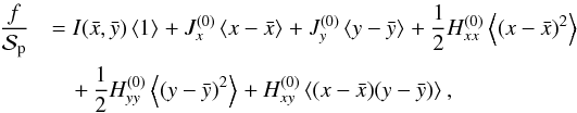 (32)where
for any function f(x,y),
(32)where
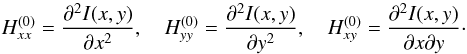
for any function f(x,y), 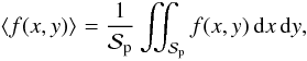 (33)where
 and
and
 are the components of the
Jacobian of the surface intensity I(x,y) computed at
.
Similarly, the components of the Hessian are
are the components of the
Jacobian of the surface intensity I(x,y) computed at
.
Similarly, the components of the Hessian are
 (34)By construction,
 and
and  are defined by
  ,
and
,
and  .
Thus, the linear terms in factor of the Jacobian
.
Thus, the linear terms in factor of the Jacobian  cancel in (32). At that point, only
 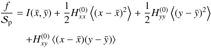 (35)remains.
The first term in (35) corresponds to the
rough approximation derived in Eq. (30).
The other terms provide a correction proportional to the square of the normalized planet
radius
(r = Rp/R⋆)
and are expected to be small.
(35)remains.
The first term in (35) corresponds to the
rough approximation derived in Eq. (30).
The other terms provide a correction proportional to the square of the normalized planet
radius
(r = Rp/R⋆)
and are expected to be small.
4.2. Subplanet velocity
The above method applied to I(x,y) to get the flux
fraction f can be adapted to any other function. For example, the
subplanet velocity is defined by 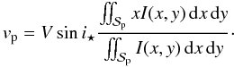 (36)We denote
 ,
,
 ,
and
,
and  as the components of the Hessian of xI(x,y) at the
averaged position
(31). Using the expression of
f (35), at first order
in r2, we get
as the components of the Hessian of xI(x,y) at the
averaged position
(31). Using the expression of
f (35), at first order
in r2, we get 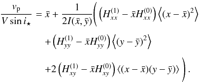 (37)The
denominator
(37)The
denominator  in (37), as well as the terms in
 ,
,
 ,
and
,
and  ,
come from the expansion of the denominator of (36).
,
come from the expansion of the denominator of (36).
4.3. Width of the subplanet line profile
The width of the subplanet line profile βp is a combination
of the width of the nonrotating line profile β0 and a
correction δβp due to the rotational
broadening  (38)We define
 as the average of the square of the subplanet velocity
  (39)With this
notation, we have
(39)With this
notation, we have  (40)Noting
 ,
,
 ,
and
,
and  ,
the components of the Hessian of
x2I(x,y) at the averaged
coordinates ,
the expression of
reads as
,
the components of the Hessian of
x2I(x,y) at the averaged
coordinates ,
the expression of
reads as 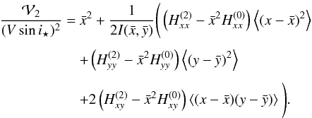 (41)At
first order, the
(41)At
first order, the  in
(39) cancels with the square of
in the expression of vp (37). Thus, at first order,
δβp vanishes and the width of the subplanet
profile is equal to the width of the nonrotating star β0.
However, the quadratic terms do not cancel, and this provides an estimation of the
contribution of the rotational broadening to the actual width of the subplanet profile.
in
(39) cancels with the square of
in the expression of vp (37). Thus, at first order,
δβp vanishes and the width of the subplanet
profile is equal to the width of the nonrotating star β0.
However, the quadratic terms do not cancel, and this provides an estimation of the
contribution of the rotational broadening to the actual width of the subplanet profile.
4.4. Limb-darkening and its derivatives
As we saw above, the determination of the subplanet profile depends on the limb-darkening
law and its second derivatives. In this section, we provide generic formulas assuming that
the limb-darkening law is a linear combination of functions
Iα(x,y) defined by
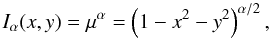 (42)where
 is the cosine of the angle between the normal of the stellar surface at
(x,y) and the observer.
is the cosine of the angle between the normal of the stellar surface at
(x,y) and the observer.
The second derivatives  ,
,
 ,
and
,
and  of
xnIα(x,y)
are given Table 1. These are the ones that are
needed to compute the flux fraction f, the subplanet velocity
vp and the dispersion βp. In
practice, only the cases n = 0,1,2 are
used.
of
xnIα(x,y)
are given Table 1. These are the ones that are
needed to compute the flux fraction f, the subplanet velocity
vp and the dispersion βp. In
practice, only the cases n = 0,1,2 are
used.
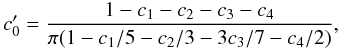
From these general formulas, one can derive the expressions for the quadratic
limb-darkening which reads as 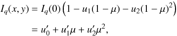 (43)with
Iq(0) the central intensity such that
Iq(x,y) is normalized to
one. By identification, we get
(43)with
Iq(0) the central intensity such that
Iq(x,y) is normalized to
one. By identification, we get  (44)Equivalently,
the so-called nonlinear limb-darkening is usually expressed as
(44)Equivalently,
the so-called nonlinear limb-darkening is usually expressed as
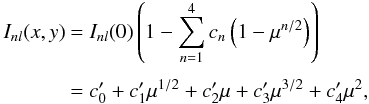 (45)with
 (46)and for
1 ≤ n ≤ 4,
(46)and for
1 ≤ n ≤ 4, 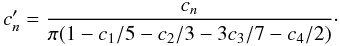 (47)The
normalizations in (44), (46), and (47) have been deduced from the integral of each
Iα(x,y) over the entire
disk of the star
(47)The
normalizations in (44), (46), and (47) have been deduced from the integral of each
Iα(x,y) over the entire
disk of the star 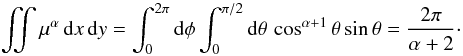 (48)
(48)
4.5. Averaged coordinates and covariances
The last quantities that need to be computed in order to get the subplanet line profiles
are the averaged coordinates  ,
,
 , the
variances
, the
variances  ,
,
 ,
and the covariance
,
and the covariance  .
For that, we distinguish two cases.
.
For that, we distinguish two cases.
4.5.1. During a full transit
In the case of a full transit, i.e., when the disk of the planet is fully inside the
disk of the star, the problem gets simpler since the integrals (33) have to be computed over a uniform disk
of area  and centered on the coordinates
(x0,y0) of
the planet. We get
and centered on the coordinates
(x0,y0) of
the planet. We get  ,
and
,
and  (49)
(49)
4.5.2. During ingress or egress
If the disk of the planet is crossing the limb of the star, the area where the integrals of the form (33) are computed is not circular (see the shaded area in Fig. 2). In that case, we use the very powerful method of Pál (2012), which gives expressions that also work also for mutual transits.
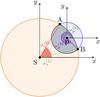 |
Fig. 2 Definition of the angles |
We recall briefly the method that relies on Green’s theorem converting an integral over
a surface into an integral over the contour of that surface:  (50)In this equation,
 is the boundary of
  ,
and ω(x,y) the exterior derivative of
f(x,y) = (fx,fy)
defined by
,
and ω(x,y) the exterior derivative of
f(x,y) = (fx,fy)
defined by  (51)When the planet is
crossing the limb of the star, the boundary is the union of two circular arcs. One of
them follows the edge of the planet centered on
(x0,y0) with
radius r. The coordinates of any points of this arc and the tangent
vectors are of the form
(51)When the planet is
crossing the limb of the star, the boundary is the union of two circular arcs. One of
them follows the edge of the planet centered on
(x0,y0) with
radius r. The coordinates of any points of this arc and the tangent
vectors are of the form  (52)The
angle ϕ varies between two limits
(52)The
angle ϕ varies between two limits
 and
and
 ,
corresponding to the intersections A and B between the
circumferences of the planet and of the star, respectively (see Fig. 2). The second arc fellows the edge of the star and is
parameterized by the coordinates
,
corresponding to the intersections A and B between the
circumferences of the planet and of the star, respectively (see Fig. 2). The second arc fellows the edge of the star and is
parameterized by the coordinates
 (53)with
ϕ going from
(53)with
ϕ going from  to
to
 associated to the intersections B and A, respectively.
More generally, if we denote
(xj,yj)j = p,s
as the centers of the arcs, and
(rj)j = p,s
as their radii such that  (54)we obtain (Pál 2012)
 (55)Here,
we are interesting in the cases where ω(x,y) stands
for 1, x, y, x2,
y2, or xy. The field vectors
f(x,y) associated to those
ω(x,y) are not uniquely determined. We choose
(55)Here,
we are interesting in the cases where ω(x,y) stands
for 1, x, y, x2,
y2, or xy. The field vectors
f(x,y) associated to those
ω(x,y) are not uniquely determined. We choose
 , (− xy,0),
(0,xy), (− x2y,0),
(0,xy2), and
, (− xy,0),
(0,xy), (− x2y,0),
(0,xy2), and
 ,
respectively. We denote
ωij = xiyj
and fij(x,y)
as the functions whose exterior derivative is
ωij. The integral of
fij along a circular arc
reads as
,
respectively. We denote
ωij = xiyj
and fij(x,y)
as the functions whose exterior derivative is
ωij. The integral of
fij along a circular arc
reads as  (56)Since
the fij are polynomials in
x and y, the
Fij can be computed using the
recurrence relations provided by Pál (2012). The
results are displayed in Table 2 for
i = 0,1,2, and
j = 0,1,2. From them, one can
derive the quantities present in the expressions of the flux fraction
f, the subplanet velocity vp and the width
βp:
(56)Since
the fij are polynomials in
x and y, the
Fij can be computed using the
recurrence relations provided by Pál (2012). The
results are displayed in Table 2 for
i = 0,1,2, and
j = 0,1,2. From them, one can
derive the quantities present in the expressions of the flux fraction
f, the subplanet velocity vp and the width
βp:
 (57)
(57)
5. Comparison with simulations
5.1. Transit light curve
Although it was not the main goal of this present work, in the derivation of a precise modeling of the RM effect, we obtained a new expression of the flux fraction f occulted by a planet during a transit (see Eq. (35)). In comparison to existing formulas that are exact (e.g. Mandel & Agol 2002; Pál 2012), the one of this paper relies on an expansion of the intensity in the vicinity of the averaged position of the planet. We thus expect our formulation to be less precise.
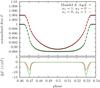 |
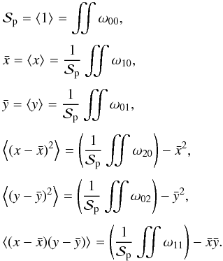
Fig. 3 Transit light curves for r = 0.1 and quadratic limb-darkening with two sets of coefficients u1, u2. The solid curves in red and in green are obtained from the approximation (35), while the black open circles are computed using the routine of Mandel & Agol (2002). |
Figure 3 shows the comparison between the approximation (35) and the exact formula derived by Mandel & Agol (2002). By eye, it is not possible to distinguish between the two approaches. In the residuals, however, we can see that the maximum of deviation occurs close to the limb, more exactly, when the edge of the planet is tangent to that of the star. Indeed, at the border of the star, the limb-darkening becomes steeper and steeper, and the derivatives ∂xIα(x,y) and ∂yIα(x,y) even go to infinity for α < 2. Nevertheless, this singularity is smoothed out by the decrease in the overlapping area between the planet and the star disks during ingress and egress.
One advantage of the present formula is that it can be easily generalized to more complex problems, as in the cases of a distorted planet, distorted star, important gravity limb-darkening, and so on. For our purpose, it provides an accurate enough estimation of the flux that can be used to derive the RM effect.
5.2. Subplanet profile
We checked the accuracy of our new formulas of the subplanet velocity
vp (37) and
the width  with
δβp given by (40). For that, we used the software called SOAP, for Spot Oscillation
And Planet (Boisse et al. 2012), to produce
artificial data as close as possible to real observations. This code is a numerical tool
that models radial velocity and photometry observations of stars with spots. It has been
updated recently to also model the effect of a planet transiting a spotted star, and was
renamed SOAP-T (Oshagh et al. 2013). Briefly, the
code divides the disk of the star into a grid. To each cell of that grid, a Gaussian
profile with a width β0 and amplitude
I(x,y) (in our notation) is assigned. This represents
the intrinsic line profile of the nonrotating star as detected by the instrument. These
lines are then shifted in velocity according to their position with respect to the
spin-axis and the Vsini⋆
of the star. All the lines of the cells uncovered by any spots or planets are added
together to produce an artificial CCF that is then fitted by a Gaussian to derive a radial
velocity.
with
δβp given by (40). For that, we used the software called SOAP, for Spot Oscillation
And Planet (Boisse et al. 2012), to produce
artificial data as close as possible to real observations. This code is a numerical tool
that models radial velocity and photometry observations of stars with spots. It has been
updated recently to also model the effect of a planet transiting a spotted star, and was
renamed SOAP-T (Oshagh et al. 2013). Briefly, the
code divides the disk of the star into a grid. To each cell of that grid, a Gaussian
profile with a width β0 and amplitude
I(x,y) (in our notation) is assigned. This represents
the intrinsic line profile of the nonrotating star as detected by the instrument. These
lines are then shifted in velocity according to their position with respect to the
spin-axis and the Vsini⋆
of the star. All the lines of the cells uncovered by any spots or planets are added
together to produce an artificial CCF that is then fitted by a Gaussian to derive a radial
velocity.
With SOAP-T, we produced the CCF of a star with a transiting planet at different positions of the planet on the disk. We also generated the CCF of the same star while the planet is not transiting, and by taking the difference, we got the subplanet profile. Such profiles are displayed in Fig. 4 for different values of Vsini⋆. Unless specified explicitly, here, and in all the following simulations, the star is a solar-type star with a quadratic limb-darkening law whose coefficients are u1 = 0.38, u2 = 0.3, and an intrinsic line width without rotation of β0 = 3 km s-1. The planet is a Jupiter evolving in the equatorial plane of its star, its radius is r = Rp/Rstar = 0.1099. In Fig. 4, the subplanet line profiles of low rotating stars are Gaussian. This results from the hypothesis of SOAP-T, which assumes Gaussian intrinsic line profiles. But we observe that the Gaussian shape holds even for Vsini⋆ = 20 km s-1, which validates our assumption leading to Eq. (14).
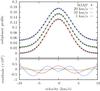 |
Fig. 4 Example of subplanet line profiles obtained with SOAP-T (circles), compared with Gaussian profiles (curves) for different stellar Vsini⋆. |
To each of the artificial subplanet profiles generated with SOAP-T, we also computed the mean velocity vp and the dispersion βp, to be compared with our formulas (37) and (40). Figure 5 shows the results for vp after normalization to remove the effect of the Vsini⋆ of the star. We checked that the figure is indeed unchanged up to Vsini⋆ = 20 km s-1. The numerical outputs obtained with SOAP-T are plotted against two different analytical approximations denoted S0 and S2. In S0, the surface brightness of the star is taken uniform below the disk of the planet, while in S2, the second derivatives are taken into account as in (37). We observe that where the error is maximal, close to the limb, S2 improves the determination of vp by about a factor 3 with respect to S0. In the case r = 0.1 and Vsini⋆ = 10 km s-1, the maximal error provided by S2 is about 20 m/s which represents a relative difference of 0.2%.
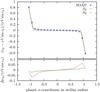 |
Fig. 5 Subplanet velocity vp produced with SOAP-T (blue points), approximation S0 assuming uniform intensity below the disk of the planet (red curve), and approximation S2 taking the second derivatives of the stellar surface brightness into account, Eq. (37) (green curve). |
In the case of the dispersion βp, the difference between the
estimation derived assuming uniform (S0) and nonuniform
(S2) brightness below the planet disk is more evident (see
Fig. 6). Indeed, in the former case,
βp remains constant and equal to the width
β0 of the nonrotating star line profile, while we observe
that for the simulated and the modeled line profiles, the shape of
βp as a function of the orbital phase looks like a trapezoid
with the large base at β0 and the maximum at approximately
 .
.
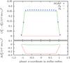 |
Fig. 6 Subplanet dispersion βp produced with SOAP-T (blue points), approximation S0 (red curve), and approximation S2, Eq. (40), (green curve). |
5.3. Rossiter-McLaughlin effect
We now compare our analytical expression of the Rossiter-McLaughlin effect vCCF (14) with signals generated with SOAP-T, which simulates the reduction analysis of the CCF technique numerically.
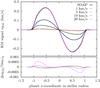 |
Fig. 7 RM signals produced with SOAP-T (solid black curves) for different Vsini⋆, and results of vCCF (14) (different dashed curves). |
Figure 7 displays the results for different Vsini⋆. As long as Vsini⋆ is below or equal to 10 km s-1, the error induced by the analytical formula remains lower than ~1 m/s, which is close to the magnitude of the precision of RV measurements. In that case, the analytical approximations are almost indistinguishable from the numerical simulations. However, for larger Vsini⋆, the agreement between numerical signals and analytical ones is weaker. For example, when Vsini⋆ = 20 km s-1, the analytical approximation leads to a maximal error of 10 m/s, which is 5% of the amplitude of the signal. Nevertheless, it should also be noted that for fast-rotating stars the spreading of the spectral lines over the detectors decreases the precision of the measurements. In any case, the analytical expression vCCF brings a definite improvement over other formulas, which have not been designed to simulate the CCF technique as we see in the following section.
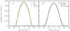 |
Fig. 8 Simple models of line profiles. a) Rotation kernel ℛ(v) with Vsini⋆ = 15 km s-1 in solid red, stellar line profile assuming β0 = 2.6 km s-1 in dashed green, subplanet line profile ℱpla(v) with βp = 2.71 km s-1 in dash-dotted blue. b) ℱtransit = ℱstar − fℱpla modeling an average line profile observed with HIRES in solid black, and a CCF observed with HARPS in dotted cyan. The same with β0 = 4.5 km s-1 and βp = 4.56 km s-1 represents a CCF observed by CORALIE, in dashed violet. |
 |
Fig. 9 Comparison of a simulated RM signal observed by different techniques and/or
instruments. We used the line profiles of Fig. 8b. The open diamonds, circles and squares represent the RM signal
obtained numerically with the iodine cell technique on the HIRES line profile, and
with the Gaussian fit to the HARPS, or CORALIE, CCFs, respectively. In a)
the gray curve corresponds to the numerical maximization of the
cross-correlation |
5.4. Comparison between different techniques
To highlight the effect of the instrument and of the data reduction analysis, we generated different models of line profile and compared the RM signals computed numerically with the results of the analytical formulas vCCF (14) and viodine (27). In our examples, the line profiles are of three types: ℱHIRES(v), ℱHARPS(v), and ℱCORALIE(v). They are associated to three RM signals: vHIRES, vHARPS, and vCORALIE, respectively. It should be stressed that the goal is not to reproduce the lines observed by those instruments exactly, but to capture their main characteristics. On the one hand, HIRES and HARPS are two spectrographs with high resolutions that we assume to be identical with a width β0 = 2.6 km s-1 for nonrotating solar-type stars. On the other hand, the resolution of CORALIE is about twice lower, and the intrinsic width of the same stars is about β0 = 4.5 km s-1 (Santos et al. 2002). We consider a star with Vsini⋆ = 15 km s-1, which is adapted to our illustration. Finally, the transiting planet is a Jupiter-like planet with a radius Rp = 0.1Rstar.
Figure 8 shows the simulated line profiles. The
panel 8a displays the rotation kernel
ℛ(v), a stellar profile ℱstar(v) with
β0 = 2.6 km s-1, and a subplanet profile
ℱpla(v − vp) multiplied by the
flux fraction f, and computed with
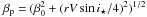 .
Figure 8b depicts the resulting line profiles
during transit ℱHIRES(v),
ℱHARPS(v), and ℱCORALIE(v).
Following our hypothesis, ℱHIRES(v) is identical to
ℱHARPS(v).
.
Figure 8b depicts the resulting line profiles
during transit ℱHIRES(v),
ℱHARPS(v), and ℱCORALIE(v).
Following our hypothesis, ℱHIRES(v) is identical to
ℱHARPS(v).
From the simulated line profiles, we derived RM signals numerically. The signal
vHIRES was obtained from ℱHIRES using the iodine
cell technique, i.e., by fitting the best Doppler shift between a line without transit
deformation, and the line profiles computed during transit. Both
vHARPS, and vCORALIE are the
results of applying the CCF technique, i.e., a numerical fit between a shifted Gaussian
and ℱHARPS and ℱCORALIE, respectively. We also generated
 by maximizing the cross-correlation
between the line profiles ℱHIRES at and out of transit. These four RM signals
are represented in Fig. 9a. It is notable that the
RM effects associated to the three instruments are all different. The variation between
vHARPS and vCORALIE is only due
to the change in resolution. However, in the case of vHIRES
and vHARPS, the simulated lines are exactly identical. The
observed difference in the RM signal is the result of the chosen data reduction technique.
Figure 9a also confirms that the maximum of the
cross-correlation
gives the same result as the iodine cell technique (when the stellar lines are
symmetrical) since
by maximizing the cross-correlation
between the line profiles ℱHIRES at and out of transit. These four RM signals
are represented in Fig. 9a. It is notable that the
RM effects associated to the three instruments are all different. The variation between
vHARPS and vCORALIE is only due
to the change in resolution. However, in the case of vHIRES
and vHARPS, the simulated lines are exactly identical. The
observed difference in the RM signal is the result of the chosen data reduction technique.
Figure 9a also confirms that the maximum of the
cross-correlation
gives the same result as the iodine cell technique (when the stellar lines are
symmetrical) since  .
.
The last three panels of Fig. 9 represent the comparison between the simulated RM signals and the analytical formulas vCCF (14), and viodine (27) associated to the CCF and the iodine cell technique, respectively. We observe that the formulas adapted to the analysis routines are in good agreement with the respective simulations. We also notice that for CORALIE, whose resolution is lower, the two analytical formulas give roughly the same result. This is because the stellar line is less affected by the rotational kernel and is more Gaussian. We show that, in that case, the two methods should indeed provide the same result (see Sect. 2.3).
From this study, we conclude that a given star observed by two different techniques should present two distinct RM signals. To date, this notable result has not been seen since the instruments with the highest signal-to-noise, HIRES and HARPS, are located in two different hemispheres. This makes it difficult to observe the same stars. For those observed with other instruments, the expected gaps are diluted by the measurement uncertainties. Nevertheless, with the advent of HARPS-North, we may observe such discrepancies in the future.
5.5. Biases on fitted parameters
As a final test, we simulated artificial data from either the CCF or the iodine cell model, and we fit each of these data with the two models separately. The goal is not to perform an exhaustive study of the biases introduced by the application of a wrong model in the process of fitting data, but to give an example with some typical parameters.
For this illustration, we considered only one set of parameters. As in the previous section, the star has Vsini⋆ = 15 km s-1 with intrinsic line width β0 = 2.6 km s-1. We chose a quadratic limb-darkening characterized by u1 = 0.69 and u2 = 0.0. The planet’s radius is taken equal to Rp = 0.1Rstar. The impact parameter of the orbit is assumed to be 0.3Rstar. For information, this value is that of a planet with a semi-major axis a = 4 Rstar and an inclination i = 85.7 deg. All these parameters were fixed throughout all the simulations. Only the projected spin-orbit angle λinput was varied from 0 to 90 degrees by steps of ten degrees. For each value of λinput, and each model, 1000 datasets were generated with a Gaussian noise of 10 m/s. Each simulation contains 50 points, among which 32 are inside the transit and 18 outside. In each case, we fit both the Vsini⋆ and the projected spin-orbit angle.
Figure 10 shows the results of this analysis in the
case where the data are generated with the CCF model vCCF
(Eq. (14)). As expected, the parameters
recovered with the appropriate model are accurate, while those deduced from the iodine
cell technique formulas are biased. The bias on
Vsini⋆ is
systematically positive and also the most important, especially at large projected
spin-orbit angle (λinput ≈ 90 deg) where we get
(Vsini⋆)fit = 20.7 ± 0.5 km s-1
instead of 15 km s-1. One can notice that this agrees with the results of,
e.g., Simpson et al. (2010) who applied the model
of Hirano et al. on WASP-3 observed with SOPHIE.
They fit a  km s-1
while the spectroscopic value is only 13.4 ± 1.5 km s-1. On the other hand, the
bias on the fitted projected spin-orbit angle λfit remains
within 2-σ. This parameter is thus less affected by the model.
km s-1
while the spectroscopic value is only 13.4 ± 1.5 km s-1. On the other hand, the
bias on the fitted projected spin-orbit angle λfit remains
within 2-σ. This parameter is thus less affected by the model.
The difference in behavior between (Vsini⋆)fit and λfit is more evident in Fig. 11. In that case, the data were simulated with the formulas associated to the iodine cell technique: viodine (Eq. (27)). As in the previous test, using the same model for both the generation of the data and the fit, leads to very accurate estimations of the parameters, while the application of the wrong model introduces biases. The (Vsini⋆)fit is systematically negative as we could expect since the situation is the opposite of the one in the previous paragraph. Nevertheless, the error is smaller. In the worst case, we get (Vsini⋆)fit = 11.9 ± 0.3 km s-1, which represents on error of the order of 3 km s-1, while it was almost 6 km s-1 in the previous example. The situation is similar for λfit. We observe small biases anticorrelated with those of the previous test, but now, the inaccuracy remains within 1-σ.
We stress that we only fit two parameters in this study, while the others are fixed to their exact values. We already observe that the best fits tend to compensate for inaccurate models by introducing biases. With more free parameters, there are more possibilities to balance the model, and it is thus difficult to predict the behavior of the fit. Since the models are not linear, we should expect the presence of several local minima. Eventually, in some of them, the projected spin-orbit angle might be more biased than in our tests. This should be analyzed on individual case bases, which is not the goal of this paper.
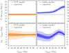 |
Fig. 10 Results of the fits with two different models of mock data generated by the CCF technique formulas. In each panel, the area with the lightest color represents the two-sigma limit, the darkest color is the one-sigma threshold, and the curve is the best value. |
6. Conclusion
One of the main objectives of this paper has been to highlight that there is no unique way of measuring RM effects and that different techniques provide different values of RV anomalies. RM signals should thus be analyzed using the appropriate model to avoid any biases, at least in Vsini⋆. This is particularly important in the case of low-impact parameters (planet passing close to the center of its star) since then, the projected spin-orbit angle only depends on the amplitude of the RM signal.
We provided a new analytical formula specially designed to model RV anomalies obtained by fitting a Gaussian function to the CCF, as in the analysis routines of HARPS and SOPHIE. We also revisited the modeling of the iodine cell technique, as used with HDS and HIRES, for which we derived an analytical expression adapted to non-Gaussian stellar line profiles. An effort was made to model the effect of the rotation of the star on the width of the subplanet line profile. Since our formulas do not rely on any expansion in powers of the subplanet velocity vp, our results remain stable even for fast-rotating stars.
The advantage of having a purely analytical expression to model the RM effect is the rapidity of computation. It can thus be used to analyze a large sample of RM signals uniformly. As a complement to this paper, we make our code accessible to the community as a free open source software package. This is a library called ARoME, an acronym for Analytical Rossiter-McLaughlin Effect, designed to generate analytical RM signals based on the formulas of the paper. It also includes the effect of macro-turbulence as described in the Appendix A. The library provides a C interface and, optionally, a Fortran 77 or 2003 interface to be called by an application. The fully documented package can be downloaded from the webpage http://www.astro.up.pt/resources/arome.
Besides the modeling of the RM effect, we also analytically derived a new expression for transit light curves (35). Although this expression is the result of a Taylor expansion of the intensity and is only adapted to small planets, it gives good approximations. Moreover, the expression is general enough to be easily extended to more complex problems.
Here, and throughout the paper, the line profiles are expressed as a function of radial velocity v, instead of wavelength.
In this paper, unit Gaussians are defined by  , while in (Hirano et al. 2010), they are defined by
 . There is thus a
difference of a factor 2 in the parenthesis of Eq. (2) with respect to (Hirano et al.
2010, Eq. (36)).
. There is thus a
difference of a factor 2 in the parenthesis of Eq. (2) with respect to (Hirano et al.
2010, Eq. (36)).
Acknowledgments
We thank Amaury Triaud for helpful discussions and feedback on this project. We also acknowledge the support by the European Research Council/European Community under the FP7 through Starting Grant agreement number 239953, as well as from Fundação para a Ciência e a Tecnologia (FCT) in the form of grant reference PTDC/CTE-AST/098528/2008. NCS also acknowledges the support from FCT through program Ciência 2007 funded by FCT/MCTES (Portugal) and POPH/FSE (EC). MM and IB would furthermore like to thank the FCT for fellowships SFRH/BPD/71230/2010 and SFRH/BPD/81084/2011, respectively.
References
- Albrecht, S., Winn, J. N., Johnson, J. A., et al. 2012, ApJ, 757, 18 [NASA ADS] [CrossRef] [Google Scholar]
- Baranne, A., Queloz, D., Mayor, M., et al. 1996, A&AS, 119, 373 [NASA ADS] [CrossRef] [EDP Sciences] [Google Scholar]
- Beaugé, C., & Nesvorný, D. 2012, ApJ, 751, 119 [NASA ADS] [CrossRef] [Google Scholar]
- Boisse, I., Bonfils, X., & Santos, N. C. 2012, A&A, 545, A109 [NASA ADS] [CrossRef] [EDP Sciences] [Google Scholar]
- Bundy, K. A., & Marcy, G. W. 2000, PASP, 112, 1421 [NASA ADS] [CrossRef] [Google Scholar]
- Butler, R. P., Marcy, G. W., Williams, E., et al. 1996, PASP, 108, 500 [NASA ADS] [CrossRef] [Google Scholar]
- Fabrycky, D., & Tremaine, S. 2007, ApJ, 669, 1298 [NASA ADS] [CrossRef] [Google Scholar]
- Giménez, A. 2006, ApJ, 650, 408 [NASA ADS] [CrossRef] [Google Scholar]
- Gray, D. F. 2005, The Observation and Analysis of Stellar Photospheres (New York, NY, USA: Cambridge University Press) [Google Scholar]
- Hébrard, G., Bouchy, F., Pont, F., et al. 2008, A&A, 488, 763 [NASA ADS] [CrossRef] [EDP Sciences] [Google Scholar]
- Hirano, T., Suto, Y., Taruya, A., et al. 2010, ApJ, 709, 458 [NASA ADS] [CrossRef] [Google Scholar]
- Hirano, T., Suto, Y., Winn, J. N., et al. 2011, ApJ, 742, 69 [NASA ADS] [CrossRef] [Google Scholar]
- Holt, J. 1893, Astronomy and Astro-Physics, XII, 646 [Google Scholar]
- Kopal, Z. 1942, Proc. Nat. Acad. Sci., 28, 133 [NASA ADS] [CrossRef] [MathSciNet] [Google Scholar]
- Mandel, K., & Agol, E. 2002, ApJ, 580, L171 [NASA ADS] [CrossRef] [Google Scholar]
- McLaughlin, D. B. 1924, ApJ, 60, 22 [NASA ADS] [CrossRef] [Google Scholar]
- Nagasawa, M., & Ida, S. 2011, ApJ, 742, 72 [NASA ADS] [CrossRef] [Google Scholar]
- Naoz, S., Farr, W. M., Lithwick, Y., Rasio, F. A., & Teyssandier, J. 2011, Nature, 473, 187 [NASA ADS] [CrossRef] [Google Scholar]
- Ohta, Y., Taruya, A., & Suto, Y. 2005, ApJ, 622, 1118 [NASA ADS] [CrossRef] [Google Scholar]
- Oshagh, M., Boisse, I., Boué, G., et al. 2013, A&A, 549, A35 [NASA ADS] [CrossRef] [EDP Sciences] [Google Scholar]
- Pál, A. 2012, MNRAS, 420, 1630 [NASA ADS] [CrossRef] [Google Scholar]
- Pepe, F., Mayor, M., Galland, F., et al. 2002, A&A, 388, 632 [NASA ADS] [CrossRef] [EDP Sciences] [Google Scholar]
- Press, W. H., Teukolsky, S. A., Vetterling, W. T., & Flannery, B. P. 1992, Numerical recipes in C (2nd ed.): the art of scientific computing (New York, NY, USA: Cambridge University Press) [Google Scholar]
- Queloz, D., Eggenberger, A., Mayor, M., et al. 2000, A&A, 359, L13 [NASA ADS] [Google Scholar]
- Rasio, F. A., & Ford, E. B. 1996, Science, 274, 954 [NASA ADS] [CrossRef] [PubMed] [Google Scholar]
- Rossiter, R. A. 1924, ApJ, 60, 15 [NASA ADS] [CrossRef] [Google Scholar]
- Santos, N. C., Mayor, M., Naef, D., et al. 2002, A&A, 392, 215 [NASA ADS] [CrossRef] [EDP Sciences] [Google Scholar]
- Simpson, E. K., Pollacco, D., Hébrard, G., et al. 2010, MNRAS, 405, 1867 [NASA ADS] [Google Scholar]
- Triaud, A. H. M. J. 2011, A&A, 534, L6 [NASA ADS] [CrossRef] [EDP Sciences] [Google Scholar]
- Triaud, A. H. M. J., Collier Cameron, A., Queloz, D., et al. 2010, A&A, 524, A25 [NASA ADS] [CrossRef] [EDP Sciences] [Google Scholar]
- Winn, J. N., Johnson, J. A., Fabrycky, D., et al. 2009, ApJ, 700, 302 [NASA ADS] [CrossRef] [Google Scholar]
- Winn, J. N., Fabrycky, D., Albrecht, S., & Johnson, J. A. 2010, ApJ, 718, L145 [NASA ADS] [CrossRef] [Google Scholar]
- Wu, Y., & Lithwick, Y. 2011, ApJ, 735, 109 [NASA ADS] [CrossRef] [Google Scholar]
- Wu, Y., & Murray, N. 2003, ApJ, 589, 605 [NASA ADS] [CrossRef] [EDP Sciences] [Google Scholar]
Appendix A: Macro-turbulence
Here, we study the effect of macro-turbulence on the Rossiter-McLaughlin signal. We
consider only the “radial-tangential” model as in (Hirano
et al. 2011). In that case, if we denote ℱ0(v) as the
line profile of the nonrotating star without macro-turbulence, the subplanet line profile
reads as , \label{eq.FplaM} \end{equation}](/articles/aa/full_html/2013/02/aa20146-12/aa20146-12-eq275.png) (A.1)where
M(v) is the rotation-turbulence kernel given by (Gray 2005),
(A.1)where
M(v) is the rotation-turbulence kernel given by (Gray 2005),
 (A.2)and
 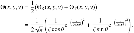 (A.3)We
highlight the different dependencies on (x,y), on the one hand, through
(A.3)We
highlight the different dependencies on (x,y), on the one hand, through
 and
and  ,
and on the velocity v, on the other. The coordinates
(x,y) are normalized by the radius of the star. Since Θ is the sum of
two Gaussians ΘR and ΘT associated to the radial and the tangential
broadenings, respectively, we also split M(v) into two
parts
,
and on the velocity v, on the other. The coordinates
(x,y) are normalized by the radius of the star. Since Θ is the sum of
two Gaussians ΘR and ΘT associated to the radial and the tangential
broadenings, respectively, we also split M(v) into two
parts  (A.4)such that
MR(v) is associated to ΘR, and
MT(v) is associated to ΘT.
(A.4)such that
MR(v) is associated to ΘR, and
MT(v) is associated to ΘT.
Now, we compute the moments of
(Mj(v))j = R,T
as in Sect. 4 to evaluate the effect of the
rotation-turbulence kernel on the subplanet profile. We have 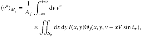 (A.5)where
Aj is a normalization constant whose
expression is
(A.5)where
Aj is a normalization constant whose
expression is 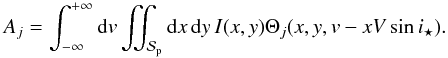 (A.6)Inverting the
integrals, we get, for the normalization,
(A.6)Inverting the
integrals, we get, for the normalization,
 (A.7)Since
Θj(x,y,v) (A.3) is normalized, the inner integral on the velocity is one. It thus
remains only
(A.7)Since
Θj(x,y,v) (A.3) is normalized, the inner integral on the velocity is one. It thus
remains only 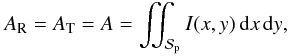 (A.8)as in Sect. 4. We now focus on the numerator of (A.5). By construction,
 . Then,
using the inversion of integrals, we get
. Then,
using the inversion of integrals, we get
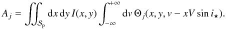
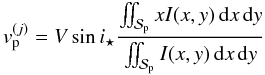
![Mathematical equation: \appendix \setcounter{section}{1} \begin{eqnarray} v_{\rm p}^{(j)} := \moy{M_j}{v} &=& \frac{1}{A} \iint_{\Spla} {\rm d}x\,{\rm d}y\,\bigg[I(x,y) \notag\\ && \times\, \int_{-\infty}^{+\infty} {\rm d}v\,v\, \Theta_j(x,y,v-xV\sin i_\star) \bigg] . \end{eqnarray}](/articles/aa/full_html/2013/02/aa20146-12/aa20146-12-eq295.png) (A.9)The
inner integral over the velocity v gives
xVsini⋆, we have thus
(A.9)The
inner integral over the velocity v gives
xVsini⋆, we have thus
 (A.10)for
each broadening: radial (j = R) and tangential
(j = T). This is identical to (36). Finally, the second moment reads as
(A.10)for
each broadening: radial (j = R) and tangential
(j = T). This is identical to (36). Finally, the second moment reads as
![Mathematical equation: \appendix \setcounter{section}{1} \begin{equation} \EQM{ {\cal V}_2^{(j)} := \moy{M_j}{v^2} = \frac{1}{A} &\iint_{\Spla} {\rm d}x\,{\rm d}y\, \bigg[ I(x,y) \crm & \times \int_{-\infty}^{+\infty} {\rm d}v\,v^2\Theta_j(x,y,v-xV\sin i_\star)\bigg] . } \end{equation}](/articles/aa/full_html/2013/02/aa20146-12/aa20146-12-eq300.png) (A.11)The
inner integral gives
(A.11)The
inner integral gives 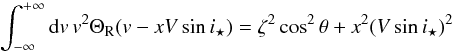 (A.12)for the
radial broadening, and
(A.12)for the
radial broadening, and 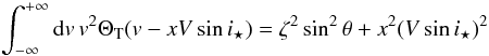 (A.13)for the
tangential broadening. We thus have
(A.13)for the
tangential broadening. We thus have
 (A.14)with
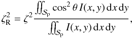 (A.15)
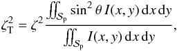 (A.16)where
corresponds to the case without macro-turbulence (Eq. (39)). It should be noted that
(A.16)where
corresponds to the case without macro-turbulence (Eq. (39)). It should be noted that  . Let
β0 be the dispersion of ℱ0(v),
and δβp the dispersion due to the rotational
broadening alone (40). The subplanet line
profile ℱpla (A.1) can be
approximated by the sum of two Gaussian functions
. Let
β0 be the dispersion of ℱ0(v),
and δβp the dispersion due to the rotational
broadening alone (40). The subplanet line
profile ℱpla (A.1) can be
approximated by the sum of two Gaussian functions
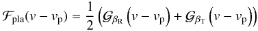 (A.17)centered
on the same value vp with respective dispersions
(A.17)centered
on the same value vp with respective dispersions
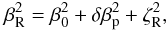 (A.18)and
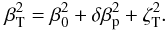 (A.19)In this expressions,
δβp, ζR, and
ζT are functions of the position of the planet on the
stellar disk. With this model, the Rossiter-McLaughlin effect, as measured by the Gaussian
fit of the CCF, reads as
(A.19)In this expressions,
δβp, ζR, and
ζT are functions of the position of the planet on the
stellar disk. With this model, the Rossiter-McLaughlin effect, as measured by the Gaussian
fit of the CCF, reads as 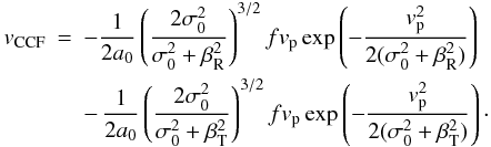 (A.20)
Appendix B: Normalization factor of the Gaussian fit
B.1. Without macro-turbulence
Here we detail the computation of the amplitude a0 of the
best Gaussian fit (13). In a first step
we neglect the macro-turbulence and have
 , \end{equation}](/articles/aa/full_html/2013/02/aa20146-12/aa20146-12-eq313.png) (B.1)with
ℱstar = ℱ0 ∗ ℛ and ℛ is the normalized rotation kernel (B.14). If we assume that ℱ0 is
Gaussian with dispersion β0, the associativity of the
convolution product leads to
(B.1)with
ℱstar = ℱ0 ∗ ℛ and ℛ is the normalized rotation kernel (B.14). If we assume that ℱ0 is
Gaussian with dispersion β0, the associativity of the
convolution product leads to  \crm & = 2\sigma_0 \sqrt{\pi} \int_{-V\sin i_\star}^{V\sin i_\star} {\cal G}_{\sigma_t}(v) {\cal R}(v) \,{\rm d}v , } \end{equation}](/articles/aa/full_html/2013/02/aa20146-12/aa20146-12-eq317.png) (B.2)with
(B.2)with
 . Finally,
since
. Finally,
since  and ℛ(v) are even functions of v, the expression of
a0 can be slightly simplified
and ℛ(v) are even functions of v, the expression of
a0 can be slightly simplified  (B.3)The amplitude
a0 is thus given by one single integral over a finite
interval, which only has to be computed once. It can be done numerically using, for
example, the simple trapezoidal rule explained in Press
et al. (1992). In the case of quadratic limb-darkening, the result can also be
expressed explicitly as a combination of modified Bessel functions and error functions
(e.g. Hirano et al. 2010, Eq. (F5)).
(B.3)The amplitude
a0 is thus given by one single integral over a finite
interval, which only has to be computed once. It can be done numerically using, for
example, the simple trapezoidal rule explained in Press
et al. (1992). In the case of quadratic limb-darkening, the result can also be
expressed explicitly as a combination of modified Bessel functions and error functions
(e.g. Hirano et al. 2010, Eq. (F5)).
B.2. With macro-turbulence
If the macro-turbulence is taken into account, it is not anymore possible to express
the amplitude a0 as a simple integral as in Sect. B.1. This is because the rotational-macroturbulence
broadening kernel cannot be expressed as a convolution product (Gray 2005). But since a0 brings only a
small correction with respect to the Gaussian case (a0
remains close to 1), we simplify the problem and approximate the line profile of the
nonrotating star as a single Gaussian with dispersion
 given by
 (B.4)instead
of two Gaussians with dispersion β0,R and
β0,T defined by
(B.4)instead
of two Gaussians with dispersion β0,R and
β0,T defined by
 (B.5)With this
simplification, we recover the expression (B.3) where σt as to be replaced
by
(B.5)With this
simplification, we recover the expression (B.3) where σt as to be replaced
by  defined by
 ,
i.e.,
,
i.e.,  (B.6)
(B.6)
B.3. Rotation kernel
We now give the expression of the rotation kernel ℛ(v) present in the
expression of the amplitude a0 (B.3) and (B.6), without or with macro-turbulence, respectively. First, we
consider a simpler kernel ℛα(v) associated
to an intensity Iα(x,y) of
the form  (B.7)With
u = v/(Vsini⋆),
the rotation kernel (Gray 2005) reads as
(B.7)With
u = v/(Vsini⋆),
the rotation kernel (Gray 2005) reads as
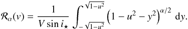 (B.8)To simplify the
integral, we make the change of variable
(B.8)To simplify the
integral, we make the change of variable  .
We obtain
.
We obtain 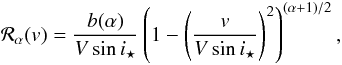 (B.9)where
 (B.10)In practice, for the
quadratic and the nonlinear limb-darkening, only the cases
α = n/2, n ∈ N
are used. The integrals b(α) can thus be computed
using the recurrence relation
(B.10)In practice, for the
quadratic and the nonlinear limb-darkening, only the cases
α = n/2, n ∈ N
are used. The integrals b(α) can thus be computed
using the recurrence relation  (B.11)with the initial
conditions
(B.11)with the initial
conditions  (B.12)The
normalized rotation kernel ℛ(v) entering in the expression of the
amplitude a0 (B.3), or (B.6), which is
associated to a normalized intensity
(B.12)The
normalized rotation kernel ℛ(v) entering in the expression of the
amplitude a0 (B.3), or (B.6), which is
associated to a normalized intensity
 (B.13)is then
 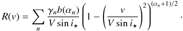 (B.14)
Appendix C: RM signal measured by the iodine cell technique
In this section, we compute an analytical expansion of
viodine (27)
modeling the RM signal measured by the iodine cell technique. The expansion is made
possible if the subplanet line profile ℱpla and that of the nonrotating star
ℱ0 are both Gaussian. In that case, if we denote
 ,
,
 ,
and ℛ(v) as the rotation kernel, we have, on the one hand,
,
and ℛ(v) as the rotation kernel, we have, on the one hand,  , \label{eq.Fstar} \end{equation}](/articles/aa/full_html/2013/02/aa20146-12/aa20146-12-eq347.png) (C.1)and, on the other hand,
(C.1)and, on the other hand,
 = \left[\frac{{\rm d}{\cal G}_{\beta_t}}{{\rm d}v}*R\right](v_{\rm p}) \label{eq.numiodine} \end{equation}](/articles/aa/full_html/2013/02/aa20146-12/aa20146-12-eq348.png) (C.2)with
(C.2)with
 . Thus, both
the numerator and the denominator involve integrals of the form
. Thus, both
the numerator and the denominator involve integrals of the form
 .
Let us consider the case where ℛ = ℛα with
.
Let us consider the case where ℛ = ℛα with
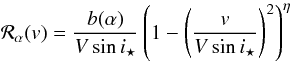 (C.3)
(C.3)
and η = (α + 1)/2. The expansion in
series of  is obtained by expanding ℛα in the vicinity of
v = 0. We have
is obtained by expanding ℛα in the vicinity of
v = 0. We have
 (C.4)where
(− η)k = 1 if k = 0, and
(− η)(− η + 1)...(− η + k − 1)
otherwise, is the Pochhammer symbol. It should be noted that if η ∈ N,
(− η)η + 1 = 0, then the sum is finite and
the expansion exact. In the following, we consider only truncated sums up to an order
K, i.e., k ≤ K. We then have
(C.4)where
(− η)k = 1 if k = 0, and
(− η)(− η + 1)...(− η + k − 1)
otherwise, is the Pochhammer symbol. It should be noted that if η ∈ N,
(− η)η + 1 = 0, then the sum is finite and
the expansion exact. In the following, we consider only truncated sums up to an order
K, i.e., k ≤ K. We then have
 &=& \frac{1}{\sqrt{2\pi}\sigma}\frac{b(\alpha)}{V\sin i_\star} \sum_{k=0}^K \Bigg( \frac{(-\eta)_k}{k!}\notag \\ \times \int_{-V\sin i_\star}^{V\sin i_\star} \hspace{-5mm}& & \left(\frac{v}{V\sin i_\star}\right)^{2k} \frac{v-\vx}{\sigma^2} \exp\left(-\frac{(v-\vx)^2}{2\sigma^2}\right) \,{\rm d}v \Bigg) . \end{eqnarray}](/articles/aa/full_html/2013/02/aa20146-12/aa20146-12-eq365.png) (C.5)We
apply the change of variable
(C.5)We
apply the change of variable  ,
and set
,
and set  and
and  .
We obtain
.
We obtain  &\!=\! & \frac{1}{\sqrt{2\pi}\sigma}\frac{b(\alpha)}{V\sin i_\star} \notag \\ &&\times\sum_{k=0}^K \Bigg( \frac{(-\eta)_k}{k!} \! \! \int_{x_1}^{x_2}\! \! \left(\frac{x\sigma+\vx}{V\sin i_\star}\right)^{2k} x \e^{-x^2/2} {\rm d}x \Bigg). \end{eqnarray}](/articles/aa/full_html/2013/02/aa20146-12/aa20146-12-eq369.png) (C.6)The
parenthesis inside the integral is then expanded which leads to
(C.6)The
parenthesis inside the integral is then expanded which leads to
 = \frac{1}{\sqrt{2\pi}\sigma}\frac{b(\alpha)}{V\sin i_\star} \sum_{k=0}^K \Bigg( \frac{(-\eta)_k}{k!} \sum_{m=0}^{2k} \bpm 2k \\ m \epm \notag\\ && \times \left(\frac{\vx}{V\sin i_\star}\right)^{2k-m} \left(\frac{\sigma}{V\sin i_\star}\right)^m \int_{x_1}^{x_2} x^{m+1} \e^{-x^2/2} \,{\rm d}x \Bigg) . \end{eqnarray}](/articles/aa/full_html/2013/02/aa20146-12/aa20146-12-eq370.png) (C.7)The
expression is easier to handle when the two sums are inverted. For that, we introduce
truncated hypergeometric functions of the form
(C.7)The
expression is easier to handle when the two sums are inverted. For that, we introduce
truncated hypergeometric functions of the form
 (C.8)and
Qm(η;x)
defined by
(C.8)and
Qm(η;x)
defined by  (C.9)and
 (C.10)With
these notations, we have
(C.10)With
these notations, we have  &= & \frac{1}{\sqrt{2\pi}\sigma}\frac{b(\alpha)}{V\sin i_\star} \sum_{m=0}^{2K} \Bigg( Q_m\left(\eta; \frac{\vx}{V\sin i_\star}\right) \notag\\ && \times\, \left(\frac{\sigma}{V\sin i_\star}\right)^m \int_{x_1}^{x_2} x^{m+1} \e^{-x^2/2} \,{\rm d}x \Bigg) , \label{eq.dGconvR} \end{eqnarray}](/articles/aa/full_html/2013/02/aa20146-12/aa20146-12-eq375.png) (C.11)where
(C.11)where
 (C.12)and
 is the lower incomplete gamma
function.
is the lower incomplete gamma
function.
The formula (C.11) gives the expansion of the numerator (C.2) of viodine (27). Moreover, the denominator, which is the integral of the square of ℱ′star (C.1) can be computed by numerical integration using the same expansion. We observe numerically that the convergence of the expansion of viodine, using Eq. (C.11), is quite fast. In practice K = 4 already gives accurate results.
All Tables
All Figures
|
Fig. 1 Simplified illustration of different methods to compute the Rossiter-McLaughlin effect. vH10, viodine, and vCCF represent the result of the hypothesis made in Hirano et al. (2010), the result of the data reduction done with the iodine cell technique, and the result of the data reduction done with the CCF technique, respectively. |
| In the text | |
|
Fig. 2 Definition of the angles |
| In the text | |
|
Fig. 3 Transit light curves for r = 0.1 and quadratic limb-darkening with two sets of coefficients u1, u2. The solid curves in red and in green are obtained from the approximation (35), while the black open circles are computed using the routine of Mandel & Agol (2002). |
| In the text | |
|
Fig. 4 Example of subplanet line profiles obtained with SOAP-T (circles), compared with Gaussian profiles (curves) for different stellar Vsini⋆. |
| In the text | |
|
Fig. 5 Subplanet velocity vp produced with SOAP-T (blue points), approximation S0 assuming uniform intensity below the disk of the planet (red curve), and approximation S2 taking the second derivatives of the stellar surface brightness into account, Eq. (37) (green curve). |
| In the text | |
|
Fig. 6 Subplanet dispersion βp produced with SOAP-T (blue points), approximation S0 (red curve), and approximation S2, Eq. (40), (green curve). |
| In the text | |
|
Fig. 7 RM signals produced with SOAP-T (solid black curves) for different Vsini⋆, and results of vCCF (14) (different dashed curves). |
| In the text | |
|
Fig. 8 Simple models of line profiles. a) Rotation kernel ℛ(v) with Vsini⋆ = 15 km s-1 in solid red, stellar line profile assuming β0 = 2.6 km s-1 in dashed green, subplanet line profile ℱpla(v) with βp = 2.71 km s-1 in dash-dotted blue. b) ℱtransit = ℱstar − fℱpla modeling an average line profile observed with HIRES in solid black, and a CCF observed with HARPS in dotted cyan. The same with β0 = 4.5 km s-1 and βp = 4.56 km s-1 represents a CCF observed by CORALIE, in dashed violet. |
| In the text | |
|
Fig. 9 Comparison of a simulated RM signal observed by different techniques and/or
instruments. We used the line profiles of Fig. 8b. The open diamonds, circles and squares represent the RM signal
obtained numerically with the iodine cell technique on the HIRES line profile, and
with the Gaussian fit to the HARPS, or CORALIE, CCFs, respectively. In a)
the gray curve corresponds to the numerical maximization of the
cross-correlation |
| In the text | |
|
Fig. 10 Results of the fits with two different models of mock data generated by the CCF technique formulas. In each panel, the area with the lightest color represents the two-sigma limit, the darkest color is the one-sigma threshold, and the curve is the best value. |
| In the text | |
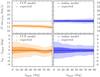 |
Fig. 11 Same as Fig. 10 but for data simulated with the iodine cell technique formulas. |
| In the text | |
Current usage metrics show cumulative count of Article Views (full-text article views including HTML views, PDF and ePub downloads, according to the available data) and Abstracts Views on Vision4Press platform.
Data correspond to usage on the plateform after 2015. The current usage metrics is available 48-96 hours after online publication and is updated daily on week days.
Initial download of the metrics may take a while.