© ESO, 2013

1. Introduction

Outflow activity is a ubiquitous phenomenon of star formation and possibly of accretion processes in general. Jets can remove angular momentum and might thereby regulate the accretion process (Matt et al. 2010, and references therein). During their early evolution, protostars are surrounded by a thick envelope and the inner parts of the outflows are usually hidden in optical and UV observations. When the envelope disperses, stars become visible in the optical as they enter the classical T Tauri stars (CTTS) phase. The outflows of CTTS can be observed very close to the central object. This allows us to investigate jet acceleration and collimation in great detail (e.g., Coffey et al. 2008). Nevertheless, the driving mechanism of these outflows remains elusive; neither the acceleration nor the collimation of outflows is understood in detail. Magneto-centrifugally launched disk winds, with a possible stellar contribution, are currently the preferred model (Pelletier & Pudritz 1992; Ferreira et al. 2006).

The CTTS DG Tau (d ≈ 140 pc, Kenyon et al. 1994) shows complex outflow-related features with stationary and moving components (the system parameters are summarized in Güdel et al. 2007). The optical jet consists of different velocity components (Bacciotti et al. 2000). Individual emission regions (knots) at greater distances from DG Tau exhibit clear proper motion (Eislöffel & Mundt 1998; Dougados et al. 2000), and Lavalley-Fouquet et al. (2000) showed that the optical forbidden emission lines (FELs) are compatible with shock heating (50 ≲ v_shock ≲ 100 km s^-1). Despite strong blueshifted C iv emission from the inner 1′′ (200 AU) around DG Tau seen in Hubble Space Telescope (HST) Goddard High-Resolution Spectrograph (GHRS) data (Ardila et al. 2002), previous HST Space Telescope Imaging Spectrograph (STIS) observations did not detect C iv emission. A non-stellar origin of the C iv emission might explain this finding because only the innermost 0$\stackrel{\mathrm{″}}{.}$1 (20 AU) were covered by STIS (Herczeg et al. 2006). DG Tau is particularly interesting since it is the only CTTS with detected stationary jet X-ray emission. This X-ray emission is located at $\mathit{d}\mathrm{\approx }\mathrm{0}\stackrel{\mathrm{″}}{.}\mathrm{2}$ (40 AU) from the driving source (Schneider & Schmitt 2008; Güdel et al. 2012). In addition to the inner, stationary X-ray component, an outer X-ray emitting knot is present, which likely possesses proper motion (Güdel et al. 2005, 2008, 2011). The jet of the class 0/I object L1551 IRS 5 shows a similar X-ray morphology (Favata et al. 2002; Schneider et al. 2011), which indicates that this phenomenon might not be exclusive to CTTS (or DG Tau).

Here we present new HST STIS observations of the DG Tau jet tracing the low temperature part (T ≈ 10³ K) with far-ultraviolet (FUV) H₂ emission, the 10⁴ K gas with specific optical FELs such as [O i], and the 10⁵ K plasma with FUV C iv and optical [O iii] emission. We also discuss the nature of the different temperature components within the innermost 150 AU.

2. Observations and data analysis

Our long-slit observations consist of a FUV spectrum covering the C iv doublet, a medium-resolution optical spectrum of important diagnostic FELs, and a blue, low-resolution spectrum (Table 1). DG Tau was positioned at the HST aimpoint, and the $\mathrm{52}″\mathrm{\times }\mathrm{0}\stackrel{\mathrm{″}}{.}\mathrm{2}$ slit was oriented along the jet axis. The FUV observations have a velocity resolution of  ≈ 25 km s^-1 (FWHM) and a spatial resolution of $\lesssim \mathrm{0}\stackrel{\mathrm{″}}{.}\mathrm{1}$ (FWHM), judging from observations of point sources with the same setup. The resolution of the optical spectra is 0.9 Å (4.1 Å) and 0$\stackrel{\mathrm{″}}{.}$13 (0$\stackrel{\mathrm{″}}{.}$15) for the G750M and G430L, respectively. All observations have nominal zero point accuracies better than $\mathrm{0}\stackrel{\mathrm{″}}{.}\mathrm{03}$ and 12 km s^-1. Velocities are expressed in the stellar rest frame as measured from the Li λ6708 line in our spectrum (+ 32 ± 2 km s^-1).

We used standard processing, i.e., the rectified flux-calibrated files and errors obtained by weighting the error instead of the variance for the FUV spectrum, which is more appropriate in the case of low-count statistics. The FUV Multi-Anode Microchannel Array (MAMA) detector suffers from several hot pixels of varying amplitudes. Visual inspection of the region around the C iv doublet shows that about ten hot pixel islands are expected in the co-added spectrum within 1543.4 Å...1554.0 Å (–1000 to +600 km s^-1 around the C iv doublet) and $\mathrm{1}\stackrel{\mathrm{″}}{.}\mathrm{2}$ to $\mathrm{-}\mathrm{0}\stackrel{\mathrm{″}}{.}\mathrm{5}$. Their flux is <4% of the total flux in this region. There is virtually no stellar light in the FUV spectra, but the C iv λ1548.2 Å line is contaminated by H₂ emission (1–8 R(3) λ 1547.3 Å); C iv λ1550.7 Å is only marginally contaminated by H₂ 2–8 P(8) λ 1550.3 Å as no line within the same fluorescence route is significantly detected (contamination  ≲5%). The H₂ contamination is about 13% of the total emission. In order to remove the H₂ contamination of the C iv emission, we subtracted the distribution of the strongest H₂ line in the same fluorescence route of the contaminating line (1–8 P(5) at 1562.4 Å) scaled by the theoretical line ratio. We removed the stellar continuum from the optical position velocity diagrams (PVDs) by measuring its intensity at line-free regions at both sides of the emission line and interpolating over the region of interest. Sampling effects caused by the tilt of the spectral trace with respect to the detector limit the accuracy of this procedure.

The inner jet’s X-ray absorption is consistent with the interstellar absorption towards the Taurus star-forming region, and we translate the X-ray absorption (N_H = 1.1 × 10²¹ cm^-2, Güdel et al. 2008) to A_V = 0.55 (E(B − V) = 0.18) using the standard conversion (Vuong et al. 2003). This leads to a transmission of 27% through the line of sight in the FUV. DG Tau itself is more strongly absorbed, both in X-rays and in the UV/optical (Güdel et al. 2007; Gullbring et al. 2000), which allowed us to separate stellar emission from jet emission in the X-ray domain. We assume a jet inclination angle of i ≈ 42°. Given errors are 90% statistical errors and do not include the effect of the spatial distribution within the slit, quoted velocities are projected ones.

3. Results

Figure 1 (top) shows the spectrum obtained around the peak of the C iv emission. The velocity-integrated spatial distributions of C iv, H₂, and [O iii] emission along the jet axis are shown in Fig. 1 (bottom). The C iv PVD is shown in Fig. 2; both C iv lines were co-added since they are compatible with the theoretical line ratio of two for optically thin emission.

3.1. Positions, sizes, and velocities

The velocity-integrated C iv flux peaks at $\mathrm{0}\stackrel{\mathrm{″}}{.}\mathrm{2}$ along the forward jet direction from DG Tau (deprojected 42 AU). The deconvolved Gaussian FWHM of the velocity-integrated C iv emission is 0$\stackrel{\mathrm{″}}{.}$25 (52 AU). Independent of the assumed flux distribution intrinsic C iv emission must be present at $\mathrm{0}\stackrel{\mathrm{″}}{.}\mathrm{05}\mathrm{-}\mathrm{0}\stackrel{\mathrm{″}}{.}\mathrm{1}$ (10–21 AU) and extend beyond $\mathrm{0}\stackrel{\mathrm{″}}{.}\mathrm{35}$ (73 AU). The spatial resolution of the X-ray observations (pixel size 0$\stackrel{\mathrm{″}}{.}$5) does not allow us a morphological comparison with hotter X-ray emitting plasma (T ≳ 3 × 10⁶ K) but the centroid of the X-ray jet is located 0$\stackrel{\mathrm{″}}{.}$14 to 0$\stackrel{\mathrm{″}}{.}$21 from DG Tau, depending on the method and observations used (the range also corresponds roughly to the statistical uncertainty). This places the C iv peak slightly (<13 AU) further away from DG Tau than the jet X-ray emission.

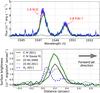Fig. 1 Top: spectrum extracted between 0$\stackrel{\mathrm{″}}{.}$15...0$\stackrel{\mathrm{″}}{.}$3. The green line describes the Gaussian fit to the C iv emission, the red curve includes the H2 contamination. Bottom: C iv and H2 flux along the jet axis summed between –400 to 0 km s-1 for the C iv emission and –80 to 0 km s-1 for the H2 lines in our FUV spectrum. Included is [O iii] λ5007 emission seen in short G430L spectra.

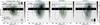Fig. 2 PVDs of important diagnostic lines with associated contours. The red dashed contour indicates the C iv emission and the horizontal dotted lines give the peak location of the two optical knots. The shaded area indicates the centroid of the inner X-ray jet (spatial extent: $\mathrm{~}\mathrm{0}\stackrel{\mathrm{″}}{.}\mathrm{1}$), the blue line visualizes the velocity of the C iv emission, and the blue contours pertain to the central jet emission in the 1999 STIS data. Contours start at 7 × 10-14 erg s-1 cm-2 Å-1 (increase by $\sqrt{\mathrm{2}}$) and at 2.5 × 10-14 erg s-1 cm-2 Å-1 (increase by a factor of 2) for C iv and optical emission, respectively.

The velocity and FWHM of the C iv emission are largest close to DG Tau and continuously decrease with increasing distance (Fig. 2). From fitting Gaussians to the C iv emission, we find that the mean velocity drops from  ≈ –180 km s^-1 at $\mathrm{0}\stackrel{\mathrm{″}}{.}\mathrm{1}$ to  ≈ –100 km s^-1 at $\mathrm{0}\stackrel{\mathrm{″}}{.}\mathrm{4}$. The FWHM drops from above  ≈ 200 km s^-1 to  ≈ 130 km s^-1 over the same region. We do not detect significant C iv emission at greater distances from DG Tau, although the STIS spectrum covers the outer X-ray emitting knot. The more strongly absorbed counter jet is also not visible in the FUV. However, both components are visible in the optical spectrum (Schneider et al., in prep.). The C iv properties are consistent with the non-detection in the less sensitive archival STIS E140M spectrum of DG Tau (Herczeg et al. 2006) because that observation covers only the inner $\mathrm{0}\stackrel{\mathrm{″}}{.}\mathrm{1}$ of the jet.

The [O iii] λ5007 emission seen in the short G430L is statistically compatible with the C iv emission. Therefore, we expect that there is no strong change in circumstellar absorption in the region where C iv emission is observed, because the ratio of FUV to optical transmission changes with increasing A_V. Another short G430L spectrum of DG Tau from the year 2000 with the slit almost aligned along the jet (PA = 230°) shows [O iii] emission with a similiar spatial distribution, but more blueshifted ($\mathrm{-}\mathrm{24}{\mathrm{9}}_{-45}^{\mathrm{+}\mathrm{27}}$ vs. $\mathrm{-}\mathrm{8}{\mathrm{8}}_{-91}^{\mathrm{+}\mathrm{119}}$ km s^-1), i.e., comparable with the C iv emission seen with GHRS. The location of [O iii] emission at $\mathrm{\approx }\mathrm{0}\stackrel{\mathrm{″}}{.}\mathrm{2}$ in two observations and the stationarity of the X-ray emission suggest that the position of the C iv emission, tracing similar temperatures as O iii, is likely also stationary.

The peak of the C iv emission corresponds to a local minimum of the H₂ emission (Fig. 1). The inner H₂ emission at $\mathrm{0}\stackrel{\mathrm{″}}{.}\mathrm{1}$ is slightly faster (30 ± 4 km s^-1) than the outer component at $\mathrm{0}\stackrel{\mathrm{″}}{.}\mathrm{3}$ (20 ± 6 km s^-1), with no significant difference in their mean FWHM of about 43 ± 8 km s^-1.

The low-temperature optical FELs [O i], [N ii], and [S ii] resemble the two H₂ components at considerably higher velocities; their PVDs (Fig. 2) show a low-velocity component (LVC, v ≈ 60 km s^-1) at $\mathrm{0}\stackrel{\mathrm{″}}{.}\mathrm{1}$ and a medium-velocity component (MVC, v ≈ 130 km s^-1) at $\mathrm{0}\stackrel{\mathrm{″}}{.}\mathrm{3}$. This structure would appear like an acceleration if both components were unresolved, but velocity and FWHM of the MVC decrease after $\mathrm{0}\stackrel{\mathrm{″}}{.}\mathrm{3}$. The C iv emission is located mainly between the LVC and MVC, but with higher velocities. The central-slit data of the 1999 STIS observation (slit-width 0$\stackrel{\mathrm{″}}{.}$1, Bacciotti et al. 2000) show low-velocity material at $\mathrm{\approx }\mathrm{0}\stackrel{\mathrm{″}}{.}\mathrm{1}$ from DG Tau, i.e., at the same position as the 2011 LVC. Additionally, the 1999 STIS data show FEL emission at $\mathrm{0}\stackrel{\mathrm{″}}{.}\mathrm{1}$ with velocities corresponding roughly to those of the 2011 C iv emission. Assuming that the higher velocity material seen 1999 in optical FELs represents the same transient part of the jet as the 2011 MVC, it is reasonable to attribute the inner LVC at $\mathrm{\approx }\mathrm{0}\stackrel{\mathrm{″}}{.}\mathrm{1}$ to stationary emission, as suggested by Lavalley et al. (1997), who compared two epochs of ground-based observations.

3.2. Fluxes, emission measure, and densities

The total C iv flux is (2.0 ± 0.1) × 10^-14 erg s^-1 cm^-2 (1548 Å + 1551 Å). The [O iii] λ5007 flux is $\mathrm{1.}{\mathrm{9}}_{-0.6}^{\mathrm{+}\mathrm{1.4}}\mathrm{\times }{\mathrm{10}}^{-14}$ erg s^-1 cm^-2. For the adapted A_V (see Sect. 1), the dust extinction corrected luminosities are L_C IV ≈ (1.8 ± 0.2) × 10²⁹   erg s^-1 and ${\mathit{L}}_{\mathrm{\left[}\mathrm{O}{iii}\mathrm{\right]}}\mathrm{\approx }\mathrm{\left(}{\mathrm{8}}_{-0.3}^{\mathrm{+}\mathrm{0.6}}\mathrm{\right)}\mathrm{\times }{\mathrm{10}}^{\mathrm{28}}\mathrm{erg}\hspace{0.17em}\mathrm{s}{}^{-1}$. Compared to the X-ray emission from the jet (L_X ≈ 10²⁹ erg s^-1 cm^-2), these values are of the same magnitude, but also show that more energy is emitted by the  ~10⁵ K than by the T ≳ 3 × 10⁶ K plasma. The flux in our spectrum is about half the flux seen in the 1996 GHRS spectrum ((4.4 ± 0.4) × 10^-14 erg s^-1 cm^-2, Ardila et al. 2002), but that spectrum also shows C iv emission mainly at higher velocities (v ~ −260 km s^-1) and thus deviates significantly from our data.

The C iv emission probably traces a distribution of temperatures, but the emissivity strongly peaks around 10⁵ K. Using the Mazzotta et al. (1998) ionization equilibrium and a C-abundance of 3 × 10^-4, we find a maximum radiative loss function of 6.8 × 10^-23 erg s^-1 cm³, so that the emission measure $\mathit{EM}\mathrm{=}{\mathit{L}}_{\mathrm{C} \mathrm{IV}}\hspace{0.17em}{\mathrm{\Lambda }}_{\mathrm{C} \mathrm{IV}}^{-1}\mathrm{\approx }\mathrm{2.6}\mathrm{\times }{\mathrm{10}}^{\mathrm{51}}\hspace{0.17em}\mathrm{cm}-3$(1)can be regarded as a lower limit on the required EM. Consequently, the density of the plasma assuming a uniformly emitting cylinder and a volume-filling factor f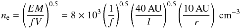${\mathit{n}}_{\mathrm{e}}\mathrm{=}{\left(\frac{\mathit{EM}}{\mathit{fV}}\right)}^{\mathrm{0.5}}\mathrm{=}\mathrm{8}\mathrm{\times }{\mathrm{10}}^{\mathrm{3}}{\left(\frac{\mathrm{1}}{\mathit{f}}\right)}^{\mathrm{0.5}}{\left(\frac{\mathrm{40}\hspace{0.17em}\mathrm{AU}}{\mathit{l}}\right)}^{\mathrm{0.5}}\left(\frac{\mathrm{10}\hspace{0.17em}\mathrm{AU}}{\mathit{r}}\right) \mathrm{cm}-3$(2)is also a lower limit (r and l are radius and length). The density sensitive [S ii] λλ 6716/6731 lines are in the critical density limit (n_crit = 2 × 10⁴ cm^-3) within the innermost $\mathrm{0}\stackrel{\mathrm{″}}{.}\mathrm{4}$ (79 AU) of the jet, i.e., at the positions of the inner knots. This density limit is comparable to that of the 10⁵ K plasma, assuming a filling factor of unity (Eq. (2)), but the [S ii] emission traces lower flowspeeds and temperatures than the C iv emission. On the other hand, the [O i] λ5577 to λ6300 ratio of 0.2 at 0$\stackrel{\mathrm{″}}{.}$1 sets a strict density limit of n < 10¹⁰ cm^-3 (cf. Fig. 12 in Hartigan et al. 1995).

4. The nature of the C IV emission

There are two possibilities for the existence of plasma exceeding T ≳ 10⁵ K within the jet at  ≈ 40 AU from DG Tau, i.e., the C iv and X-ray emitting material: either some part of the outflow is already hot close to the launching point or the jet is sufficiently heated while flowing outwards.

4.1. A hot inner outflow

First, we consider a cylindrical/conical outflow that is launched with a sufficient temperature to explain the observed spatial offsets as a result of cooling and a special absorption geometry; how such an outflow might be confined and stabilized is beyond the scope of this letter. The C iv emitting plasma has a short radiative cooling time, e.g., about one day corresponding to a length of 0.1 AU along the jet axis at v = 200 km s^-1 for n_e = 10⁶ cm^-3 (${\mathit{\tau }}_{\mathrm{rad}}\mathrm{~}{\mathit{n}}_{\mathrm{e}}^{-1}$). Therefore, the C iv emitting region must have a large extent perpendicular to the jet axis to provide the required EM. Using Eq. (2) with l = l_cool = 0.1 AU/n₆ and assuming that C iv is emitted between log T = 4.9 and 5.2, a filling factor of unity (f = 1), and a cylindrical emission region, we estimate that the radius must be r = 1.6 AU ${\mathit{n}}_{\mathrm{6}}^{-0.5}$ with n₆ density in 10⁶ cm^-3 (n_e ≈ n at the temperatures at hand). Such a wind has Ṁ = vμm_Hnπr² ≈ 10^-9   M_⊙ yr^-1. Densities around 10⁴ cm^-3 give a cooling distance comparable to the observed offset for T₀ slightly above 10⁵ K, and the peak of the C iv emission might simply denote the location where the C iv radiative losses are largest (T = 10⁵ K). However, this requires that the disk launches a wind with T > 10⁵ K over r > 10 AU and does not explain the proximity of X-ray and C iv emission. These issues can be addressed by proposing higher initial temperatures and densities, e.g., T = 3 × 10⁶ K and n_e = 10⁶ cm^-3. In this case, the X-ray emission close to DG Tau must be absorbed to explain the offset of the X-ray emission and the low X-ray to C iv ratio, since such a radiative wind has an X-ray to C iv emission ratio of  ~40 (estimated using the CHIANTI database, Dere et al. 2009). We note that the X-ray absorption of DG Tau reduces the soft X-ray transmission by a sufficient factor (~10²). On the other hand, the X-ray data exclude initial temperatures exceeding a few 10⁷ K, which would allow n ≳ 10⁷ cm^-3. Therefore, the launching radius is r ≳ 0.5 AU. The observed distribution of C iv emission along the jet might result from different densities and velocities of individual plasmoids (cf. Skinner et al. 2011), whose cooling times might be altered by thermal conduction.

The expansion of a conical wind adds an extra cooling term and thus requires higher initial temperatures. The emission measure per unit length along the jet axis is also reduced, compared to a cylindrical outflow. As a result, higher initial densities are required to produce a similar C iv luminosity compared to a radiative wind with the same intial radius. Therefore, a conical outflow does not allow smaller launching radii. We thus regard an outflow with an initial temperature well above 10⁶ K launched over r ≳ 1 AU unlikely and conclude that the heating must happen further out.

4.2. Local heating

Another possibility is that shocks locally heat the outflowing gas. Magnetic fields reduce the effective shock velocity and increase the cooling distance by limiting the compression of the post-shock plasma (Hartigan et al. 2007). For negligible magnetic fields, however, the cooling distance is very short (less than one-tenth of an AU for n_e = 10⁶ cm^-3 and v_shock = 200 km s^-1, Hartigan et al. 1987). Therefore, the observed length of the emission region along the jet axis results either from a single large oblique shock and inclination effects or from a number of small shocks at different streamlines since the observed velocities argue against a number of shocks for a single streamline.

Using the shock code of Günther et al. (2007) for negligible magnetic fields perpendicular to the shock surface, the detected (dereddened) soft X-ray luminosity of  ≈ 10²⁹ erg s^-1is insufficient to explain the C iv emission as cooled, previously X-ray-emitting plasma (a stationary 1D shock with v_shock ≈ 400 km s^-1 radiates less than 20% of its soft X-ray luminosity in C iv). Without invoking extra-absorption for the soft X-ray emission, the observed C iv emission requires additional heating, e.g., additional shocks with lower velocities, than the very high-velocity shocks responsible for the X-ray emission.

For the shock scenario, we can estimate the required mass-loss from the fraction of the post-shock gas seen in C iv (cf. estimate for O i emission in Hartigan et al. 1995). For a stationary oblique shock, the ratios of shock to jet velocity and shock to jet surface are equal and cancel out in the calculation. From the Hartigan et al. (1987) models, we estimate that every atom crossing the shock emits N ≈ 0.3 C iv photons, so that

$\mathit{Ṁ}\mathrm{=}\frac{{\mathit{L}}_{\mathrm{CIV}}}{\mathit{Nh}{\mathit{\nu }}_{\mathrm{CIV}}}\mathit{\mu }{\mathit{m}}_{\mathrm{H}}\mathrm{\approx }\mathrm{2}\mathrm{\times }{\mathrm{10}}^{-9}\left(\frac{\mathrm{0.3}}{\mathit{N}}\right)\left(\frac{{\mathit{L}}_{\mathrm{CIV}}}{\mathrm{1.8}\mathrm{\times }{\mathrm{10}}^{\mathrm{29}}\hspace{0.17em}\mathrm{erg}\hspace{0.17em}\mathrm{s}-1}\right)\hspace{0.17em}{\mathit{M}}_{\mathrm{\odot }}\hspace{0.17em}\mathrm{yr}-1.$ 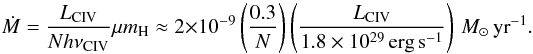This is lower than the values derived from near-IR jet tracers (Ṁ ≳ 10^-8M_⊙ yr^-1Agra-Amboage et al. 2011). Possibly only a fraction of the outflow is heated to C iv emitting temperatures.

Alternatively, the jet might be locally heated by magnetic reconnection. We utilize the fact that the magnetic field is frozen into the plasma in a sufficiently ionized gas, i.e., is co-moving with the plasma. For an order of magnitude estimate, we approximate the inflow of magnetic energy by

${\mathit{L}}_{\mathrm{mag}}\mathrm{~}{\mathit{v}}_{\mathrm{B}}{\mathit{A}}_{\mathrm{r}}\frac{{\mathit{B}}^{\mathrm{2}}}{\mathrm{8}\mathit{\pi }}\mathrm{~}{\mathrm{10}}^{\mathrm{32}}\mathrm{erg}\hspace{0.17em}\mathrm{s}-1\left(\frac{{\mathit{v}}_{\mathrm{B}}}{\mathrm{200}\hspace{0.17em}\mathrm{km}\hspace{0.17em}\mathrm{s}-1}\right){\left(\frac{{\mathit{r}}_{\mathrm{A}}}{\mathrm{10}\hspace{0.17em}\mathrm{AU}}\right)}^{\mathrm{2}}{\left(\frac{\mathit{B}}{\mathrm{50}\hspace{0.17em}\mathrm{mG}}\right)}^{\mathrm{2}}\mathit{,}$where v_B describes the velocity of the plasma component carrying the magnetic field through the area A_r (radius r_A) into the reconnection region, and we used the Hartigan et al. (2007) estimate of B at 50 AU. A luminosity of L_mag ≳ 3 × 10³⁰ erg s^-1 is required to power the C iv emitting plasma since its total radiative loss is about 15 times L_CIV. Although probably only a small fraction of L_mag is used for heating, it appears possible that magnetic heating is sufficient to heat the high-temperature plasma.

We conclude that local heating can explain the observed high-temperature plasma within the DG Tau jet. The apparent stationarity of the high-temperature plasma then requires a quasi stationary process at some distance to DG Tau. The location of the high-temperature plasma in the collimation region makes an association with oblique shocks due to collimation likely. Possibly the highest velocity shocks are closer to the jet axis and to the source, while slower shocks exist at larger distances which explains the offset between X-ray and C iv emission.

Acknowledgments

P.C.S. is supported by the DLR under grant 50OR1112. HMG is supported by NASA through Chandra Award Number GO1-12067X on behalf of NASA under contract NAS8-03060. This paper is based on observations made with the NASA/ESA Hubble Space Telescope.

References

All Tables

All Figures

Fig. 1 Top: spectrum extracted between 0$\stackrel{\mathrm{″}}{.}$15...0$\stackrel{\mathrm{″}}{.}$3. The green line describes the Gaussian fit to the C iv emission, the red curve includes the H2 contamination. Bottom: C iv and H2 flux along the jet axis summed between –400 to 0 km s-1 for the C iv emission and –80 to 0 km s-1 for the H2 lines in our FUV spectrum. Included is [O iii] λ5007 emission seen in short G430L spectra.

In the text

Fig. 2 PVDs of important diagnostic lines with associated contours. The red dashed contour indicates the C iv emission and the horizontal dotted lines give the peak location of the two optical knots. The shaded area indicates the centroid of the inner X-ray jet (spatial extent: $\mathrm{~}\mathrm{0}\stackrel{\mathrm{″}}{.}\mathrm{1}$), the blue line visualizes the velocity of the C iv emission, and the blue contours pertain to the central jet emission in the 1999 STIS data. Contours start at 7 × 10-14 erg s-1 cm-2 Å-1 (increase by $\sqrt{\mathrm{2}}$) and at 2.5 × 10-14 erg s-1 cm-2 Å-1 (increase by a factor of 2) for C iv and optical emission, respectively.

In the text

References

- Agra-Amboage, V., Dougados, C., Cabrit, S., & Reunanen, J. 2011, A&A, 532, A59 [NASA ADS] [CrossRef] [EDP Sciences] [Google Scholar]
- Ardila, D. R., Basri, G., Walter, F. M., Valenti, J. A., & Johns-Krull, C. M. 2002, ApJ, 566, 1100 [NASA ADS] [CrossRef] [Google Scholar]
- Bacciotti, F., Mundt, R., Ray, T. P., et al. 2000, ApJ, 537, L49 [NASA ADS] [CrossRef] [Google Scholar]
- Coffey, D., Bacciotti, F., & Podio, L. 2008, ApJ, 689, 1112 [NASA ADS] [CrossRef] [Google Scholar]
- Dere, K. P., Landi, E., Young, P. R., et al. 2009, A&A, 498, 915 [NASA ADS] [CrossRef] [EDP Sciences] [Google Scholar]
- Dougados, C., Cabrit, S., Lavalley, C., & Ménard, F. 2000, A&A, 357, L61 [NASA ADS] [Google Scholar]
- Eislöffel, J., & Mundt, R. 1998, AJ, 115, 1554 [NASA ADS] [CrossRef] [Google Scholar]
- Favata, F., Fridlund, C. V. M., Micela, G., Sciortino, S., & Kaas, A. A. 2002, A&A, 386, 204 [NASA ADS] [CrossRef] [EDP Sciences] [Google Scholar]
- Ferreira, J., Dougados, C., & Cabrit, S. 2006, A&A, 453, 785 [NASA ADS] [CrossRef] [EDP Sciences] [Google Scholar]
- Güdel, M., Skinner, S. L., Briggs, K. R., et al. 2005, ApJ, 626, L53 [NASA ADS] [CrossRef] [Google Scholar]
- Güdel, M., Telleschi, A., Audard, M., et al. 2007, A&A, 468, 515 [NASA ADS] [CrossRef] [EDP Sciences] [Google Scholar]
- Güdel, M., Skinner, S. L., Audard, M., Briggs, K. R., & Cabrit, S. 2008, A&A, 478, 797 [NASA ADS] [CrossRef] [EDP Sciences] [Google Scholar]
- Güdel, M., Audard, M., Bacciotti, F., et al. 2012, in 16th Cambridge Workshop on Cool Stars, Stellar Systems, and the Sun, eds. C. M. Johns-Krull et al. (San Francisco: ASP), ASP Conf. Ser., 448, 617 [Google Scholar]
- Gullbring, E., Calvet, N., Muzerolle, J., & Hartmann, L. 2000, ApJ, 544, 927 [NASA ADS] [CrossRef] [Google Scholar]
- Günther, H. M., Schmitt, J. H. M. M., Robrade, J., & Liefke, C. 2007, A&A, 466, 1111 [NASA ADS] [CrossRef] [EDP Sciences] [Google Scholar]
- Hartigan, P., Raymond, J., & Hartmann, L. 1987, ApJ, 316, 323 [NASA ADS] [CrossRef] [Google Scholar]
- Hartigan, P., Edwards, S., & Ghandour, L. 1995, ApJ, 452, 736 [NASA ADS] [CrossRef] [Google Scholar]
- Hartigan, P., Frank, A., Varniére, P., & Blackman, E. G. 2007, ApJ, 661, 910 [NASA ADS] [CrossRef] [Google Scholar]
- Herczeg, G. J., Linsky, J. L., Walter, F. M., Gahm, G. F., & Johns-Krull, C. M. 2006, ApJS, 165, 256 [NASA ADS] [CrossRef] [Google Scholar]
- Kenyon, S. J., Dobrzycka, D., & Hartmann, L. 1994, AJ, 108, 1872 [NASA ADS] [CrossRef] [Google Scholar]
- Lavalley, C., Cabrit, S., Dougados, C., Ferruit, P., & Bacon, R. 1997, A&A, 327, 671 [NASA ADS] [Google Scholar]
- Lavalley-Fouquet, C., Cabrit, S., & Dougados, C. 2000, A&A, 356, L41 [NASA ADS] [Google Scholar]
- Matt, S. P., Pinzón, G., de la Reza, R., & Greene, T. P. 2010, ApJ, 714, 989 [NASA ADS] [CrossRef] [Google Scholar]
- Mazzotta, P., Mazzitelli, G., Colafrancesco, S., & Vittorio, N. 1998, A&AS, 133, 403 [Google Scholar]
- Pelletier, G., & Pudritz, R. E. 1992, ApJ, 394, 117 [NASA ADS] [CrossRef] [Google Scholar]
- Schneider, P. C., & Schmitt, J. H. M. M. 2008, A&A, 488, L13 [NASA ADS] [CrossRef] [EDP Sciences] [Google Scholar]
- Schneider, P. C., Günther, H. M., & Schmitt, J. H. M. M. 2011, A&A, 530, A123 [NASA ADS] [CrossRef] [EDP Sciences] [Google Scholar]
- Skinner, S. L., Audard, M., & Güdel, M. 2011, ApJ, 737, 19 [NASA ADS] [CrossRef] [Google Scholar]
- Vuong, M. H., Montmerle, T., Grosso, N., et al. 2003, A&A, 408, 581 [NASA ADS] [CrossRef] [EDP Sciences] [Google Scholar]