| Issue |
A&A
Volume 549, January 2013
|
|
|---|---|---|
| Article Number | A105 | |
| Number of page(s) | 5 | |
| Section | The Sun | |
| DOI | https://doi.org/10.1051/0004-6361/201220503 | |
| Published online | 07 January 2013 | |
A solar tornado triggered by flares?⋆
1
Max-Planck Institut für Sonnensystemforschung,
Max-Planck-Str. 2,
37191
Katlenburg-Lindau,
Germany
e-mail: panesar@mps.mpg.de
2
Institut für Astrophysik, Georg-August-Universität Göttingen,
Friedrich-Hund-Platz
1, 37077
Göttingen,
Germany
3
High Altitude Observatory, National Center for Atmospheric Research, PO Box
3000, Boulder,
CO
80307,
USA
Received:
5
October
2012
Accepted:
24
November
2012
Context. Solar tornados are dynamical, conspicuously helical magnetic structures that are mainly observed as a prominence activity.
Aims. We investigate and propose a triggering mechanism for the solar tornado observed in a prominence cavity by SDO/AIA on September 25, 2011.
Methods. High-cadence EUV images from the SDO/AIA and the Ahead spacecraft of STEREO/EUVI are used to correlate three flares in the neighbouring active-region (NOAA 11303) and their EUV waves with the dynamical developments of the tornado. The timings of the flares and EUV waves observed on-disk in 195 Å are analysed in relation to the tornado activities observed at the limb in 171 Å.
Results. Each of the three flares and its related EUV wave occurred within ten hours of the onset of the tornado. They have an observed causal relationship with the commencement of activity in the prominence where the tornado develops. Tornado-like rotations along the side of the prominence start after the second flare. The prominence cavity expands with the accelerating tornado motion after the third flare.
Conclusions. Flares in the neighbouring active region may have affected the cavity prominence system and triggered the solar tornado. A plausible mechanism is that the active-region coronal field contracted by the “Hudson effect” through the loss of magnetic energy as flares. Subsequently, the cavity expanded by its magnetic pressure to fill the surrounding low corona. We suggest that the tornado is the dynamical response of the helical prominence field to the cavity expansion.
Key words: Sun: chromosphere / Sun: filaments, prominences / Sun: flares
Movies are available in electronic form at http://www.aanda.org
© ESO, 2013
1. Introduction
Prominences consist of relatively extended, cool, and overdense plasma seen in the lower corona above the solar limb (Martin 1998; Tandberg-Hanssen 1995; Mackay et al. 2010). Their structure and composition are exceedingly complicated. The plasma mainly resides in highly tangled magnetic fields (van Ballegooijen & Cranmer 2010). Coronal cavities are often observed to have cooler prominence plasma at their bases (Hudson et al. 1999; Gibson et al. 2006; Régnier et al. 2011). The cavity is a region of relatively low-density high-temperature plasma (Gibson et al. 2010; Habbal et al. 2010). Berger et al. (2011) have proposed that the prominence and its cavity are a form of magneto-thermal convective structure, macroscopically stable, but internally in a constant state of ubiquitous motions (Low et al. 2012a,b).
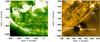 |
Fig. 1 Region around the tornado on 25 September 2011: a) EUVI-A 195 Å; b) AIA 171 Å images. On the EUVI image, the black dashed line shows the position of the AIA limb, and the long diagonal arrow is the epipolar line for the prominence position marked with + on the AIA image. The orange dashed line outlines the position of the southern edge of the active region (AR) corona. |
Viewed at the limb, quiescent prominences mostly appear as curtains of vertical thread-like structures (Berger et al. 2008). Occasionally they look like tornados with rotations along, or of, their magnetic structures (Pettit 1943; Liggett & Zirin 1984). At first glance it is not obvious why tornados do not erupt but continue to rotate for several hours before quietening down. Recently, images from the Atmospheric Imaging Assembly (AIA) on the Solar Dynamic Observatory (SDO) have allowed the study of solar tornados (Li et al. 2012; Su et al. 2012; Liu et al. 2012a). The driving mechanism may be a coupling and expansion of a twisted flux rope into the coronal cavity (Li et al. 2012) and/or be related to photospheric vortices at the footpoint of the tornado (Attie et al. 2009; Wedemeyer-Böhm et al. 2012; Su et al. 2012).
We study the impressive solar tornado observed by the AIA on 25 September 2011. Li et al. (2012) described the formation and disappearance of the related prominence by analysing SDO data from 24−26 September. The evolution of the tornado was attributed to the expansion of helical structures into the cavity. But the reason behind the expansion remained an open question.
Here we analyse observations of the mechanism that led to the expansion of the prominence. We show with Solar TErrestrial RElations Observatory (STEREO) Extreme UltraViolet Imager (EUVI) observations that three strong flares in a neighbouring active region coincided with phases of the tornado activation. Each flare was associated with a coronal mass ejection (CME) and an EUV wave. Particularly after the third flare, a slow but significant expansion of the overlying prominence cavity was observed together with more rapid rotation at the top of the prominence. We describe the observations in Sect. 2. The evolution of the tornado, its relationship to the solar flares and the EUV waves are described in Sect. 3. In Sect. 4, we summarize our observations and speculate on the link between the flares and the cavity expansion.
2. Observations
The solar tornado on 25 September 2011 was observed on the southwest limb by SDO/AIA (Lemen et al. 2012). In images from EUVI on the Ahead spacecraft of STEREO (Howard et al. 2008), it appeared on the solar disk around 15° E. The separation angle between SDO and STEREO-A was 103°. We studied the tornado with combined observations from the two directions.
The AIA takes high spatial resolution (0.6′′ pixel-1) full-disk images with a cadence of 12 s. For the analysis, we selected images from the 171 Å channel, which is centred on the Fe ix line formed around 0.63 MK. Images from this channel show the hot, bright, emitting and the cold, dense, absorbing parts of the prominence, as well as the dark, low-density cavity and the surrounding coronal loops. To enhance the visibility of the cavity and faint loops, we removed an average background from the 171 Å images by taking the median of two months of data – September and October, 2011.
During the period of 01:30−13:30 UT, SDO was in eclipse from 06:02-07:13 UT. This gap is covered by the SWAP instrument on PROBA-2 (Halain et al. 2010). SWAP provides a full Sun 174 Å image every 2−3 min with a spatial resolution of 3.16′′ pixel-1. The images are not as detailed as the AIA images, but they are essential for checking the behaviour of the prominence during the data gap.
The EUVI-A 195 Å images have a time cadence of 5 min and a resolution of 1.6′′
pixel-1. The 195 Å emission is mainly Fe xii formed at
~1.2 MK. To confirm the prominence position in the EUVI images, we obtained the
three-dimensional coordinates of the prominence with the routine
SCC MEASURE
(Thompson 2009) available in the SolarSoft library.
MEASURE
(Thompson 2009) available in the SolarSoft library.
2.1. Overview
In Fig. 1 we show the EUVI-A 195 Å and AIA 171 Å images of the filament/prominence and the active region NOAA 11303 (marked with an arrow) as seen from the two angles. The position of the cross on the stem of the prominence lies along the epipolar line drawn as a long black arrow on the EUVI image. The dark lane crossed by the epipolar line is the filament channel and the tornado is the bright region that coincides with the epipolar line and the filament channel, indicated with a black arrow. The core of the active region is separated by 300′′ from the filament channel. However, the southern edge of the active-region corona (outlined by the orange dashed line) reaches to within 50′′ of the filament channel.
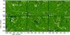 |
Fig. 2 EUVI-A 195 Å running-ratio images showing the onset of the three flares (a), b), and c)) and their associated EUV waves (d), e), and f)). In a) the epipolar line shown in Fig. 1a is drawn as a long white arrow, and the solar limb is drawn as a dashed white line. The small white arrow in all images points to the tornado site. The dot-dashed/dashed lines in b) mark the positions of time series shown in Fig. 4, and the orange dashed line along the EUV wave front in e) is the position of the time series in Fig. 3. |
2.2. The three flares
There were flares at approximately 02:45, 07:00, 09:40 UT from the nearby active region. They were all associated with CMEs and EUV waves. The third was GOES class M1.4 according to the NOAA flare catalogue1. The GOES class of the first two are not given in the catalogue. We therefore checked the hard X-ray quicklook images from the Reuven Ramaty High Energy Solar Spectroscopic Imager (RHESSI). Unfortunately, both had their peaks during RHESSI data gaps. The first RHESSI image in the flares’ decay phase showed that these flares were the brightest RHESSI sources. At the time of the first and second flares the GOES 1−8 Å fluxes reached the M4.4 and M1.0 level, so it is possible that these were M-class flares as well.
The flares’ onsets and related EUV waves can be seen in the 195 Å running ratio images shown in Fig. 2. The running ratio images are the log of the intensity at the time shown in the images divided by the intensity 5 min earlier. Because this reflects relative changes, the faint EUV waves show up against bright inactive active regions. The faint EUV wavefronts sweep over the filament channel about half an hour after the flare (bottom row). The small white arrows point to the tornado site, which showed increased activity along the filament channel after the flares.
When we take a time series along the orange dashed line drawn in Fig. 2e, we are able to see the relation between the EUV waves and the filament activity (Fig. 3). In this time series image, the waves associated with the three flares are marked by F1, F2, and F3 and a red arrow points to the filament activity. The filament activity associated with F2 increased before the arrival of the EUV wave. Further more, each EUV wave front was followed by a series of oscillations with a period of 20 min at the edge of the active region and along the filament channel. Similar post-EUV cavity oscillations, seen at the limb in the AIA images, have been reported by Liu et al. (2012b). EUVI images have a much lower cadence than those from the AIA, and may not be resolving the wave trains.
As mentioned above, the EUV wave reached the filament channel after the filament activation. To investigate whether the activation could have been triggered by the flare, we took time series through the flare sites (vertical line Fig. 2b) and along the filament channel across the activated filament (horizontal line in Fig. 2b). We observe that there are perturbations in the filament plasma immediately after each flare (yellow arrows in Fig. 4b). Large-scale changes along the filament channel started after F2 and increased further after the F3.
The reaction of the prominence to the flares is illustrated in Fig. 7. The positions of the three time series are drawn in Fig. 6, an AIA image of the active region and the tornado. The oscillations of the prominence at the time of F1 (Fig. 7a) are consistent with a flare trigger from the north since it moved first towards the pole. The wobbling in the prominence after the flare is also clearly visible in movie6a (Fig. 6).
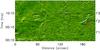 |
Fig. 3 EUVI 195 Å running-ratio space-time image along the dashed line in Fig. 2e. The three flares are labelled F1, F2, and F3. The red arrow points to the filament. |
The second flare, F2, was at ~06:45 UT when SDO was in eclipse. Since this phase is important for understanding the tornado, we checked the SWAP data to see if the prominence activation started before F2. The SWAP data are shown in the movie attached to Fig. 5. Although the SWAP images are not as sharp as the AIA images, they show quite clearly that increased prominence activity occurred after F2 and that the first AIA images after eclipse caught the expansion of the flare loops and the rapid growth in prominence activity. The middle image in Fig. 7b, taken along the dashed line in Fig. 6, shows an arm of prominence plasma that reaches out in the direction of the active region. There is also a very slight expansion of the cavity boundary towards the active region.
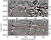 |
Fig. 4 EUVI 195 Å running-difference time-series along a) the vertical and b) the horizontal line in Fig. 2b. The red dashed lines are drawn at the times of flare F1, F2, and F3. In b) the yellow arrows point to the changes in filament structure after the flares. |
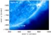 |
Fig. 5 SWAP 174 Å intensity image from 25 September 2011. The arrows show the positions of the cavity and the active region (AR). This frame is taken from the movie “MOVIE5.mp4”. |
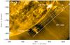 |
Fig. 6 AIA 171 Å intensity image. The diagonal long arrows show the positions of the time-series images through the prominence/tornado, cavity, active region hot loop (AR loop) and active-region (AR) shown in Fig. 7. This is the frame from the movie “MOVIE6b.mp4”. “MOVIE6a.mp4” shows the evolution of this region at earlier times. |
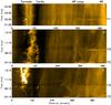 |
Fig. 7 AIA 171 Å intensity time-series along the diagonal arrows in Fig. 6: a) oscillations of the prominence stem triggered by F1 taken along the bottom white arrow; b) activity triggered by F2 and F3 taken along the middle white arrow; c) tornado activity and cavity changes triggered by F2 and F3 taken along the top arrow. The arrow at the time of the flare (~09.40 UT) points to the movement of the cavity boundary. |
The biggest change in the cavity occurred after F3 when the bright and complex top part of the prominence started to rotate faster. Movie6b, attached to Fig. 6, shows the evolution of the tornado and flare from F2 to a couple of hours after F3. The time series in Fig. 7c, taken along the top white arrow in Fig. 6, shows the main features. The flare erupted at 09:20 UT. The active-region loops started to expand at 09:40:48 UT. At 09:50:13 UT there was a sharp contraction, approximately 10 Mm, of the observed cavity. The cavity started to expand back towards the active region after ~10:00 UT. It grew from 140 Mm to 167 Mm in 3.5 h. At the same time, the prominence grew in height and the bright and complex head of the prominence started to rotate faster, forming the tornado. The rotations at the top of the prominence/tornado lasted ~3.5 h with a speed from 55 km s-1 to 95 km s-1 (Li et al. 2012).
3. Discussion
A solar tornado was observed by the AIA and EUVI-A on 25 September 2011. The tornado was reported by Li et al. (2012), who attributed it to the growth of a helical prominence system. The reason for the prominence growth remained unanswered. After careful analysis of the AIA full-disk images, we noticed that AR 11303, to the north of the prominence cavity, was flaring and suspected it of having influenced the prominence in some way. We observed three flares, which were all associated with EUV waves that swept over the prominence cavity. Each time the cavity was buffeted by the wave, the prominence plasma became more active. After the third flare a tornado had developed at the top of the prominence.
After the first flare, there were clear oscillations along the prominence stem. The second flare caused plasma to move along arm-like extensions projecting out from the stem in the direction of the active region. These extensions appear to have subsequently rotated back towards the prominence before the third flare. After the third flare the tornado became very strong and was stable for about 3.5 h. The third flare seemed to have the biggest impact on the surrounding plasma, or at least it produced the most visible (at 195 Å) EUV wave. It also caused large active-region loops to move towards the edge of the prominence cavity. Afterwards, the loops swayed back and the cavity started to slowly (~2.5 km s-1) but visibly expand over the next 3.5 h. During this time the prominence rose into the cavity and created the tornado.
To understand the relationship between the flare, the prominence, the cavity, and the tornado, several effects need to be considered. The expansion of the cavity is clearly associated with the rise of the prominence plasma. One possible explanation for the expansion is that the loss of free magnetic energy from the active region by flares and CMEs (Zhang & Low 2005) resulted in a contraction of the active region field, the Hudson effect (Hudson 2000; Zhang & Low 2003; Janse & Low 2007). Subsequently, the surrounding fields, including the cavity field, expanded to fill the vacated space.
An idealized illustration of the Hudson effect, in terms of the force-free equilibrium between two bipolar fields before and after one of the fields has lost its free energy, is given in Fig. 8. Initially, the active-region field on the right has excess free energy, and the cavity field on the left is taken to be potential to simplify the calculation. During the eruption, the active-region field loses free energy, decreasing its pressure since the magnetic energy density B2 of a field B is also the magnetic pressure. This leads to an expansion of the cavity field to restore the pressure balance in the system.
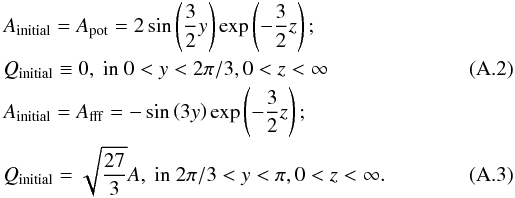
We consider the 2D Cartesian domain
0 < y < π,
0 < z < ∞, where x is an ignorable
coordinate, taking the boundary to be a rigid perfect electrical conductor for simplicity.
The initial state in Fig. 8a is a continuous global
solution for the magnetic field,
B = Binitial of the
force-free equations  (1)which describe a
bipolar (α = 0) potential field that represents the cavity that occupies
the partial domain
0 < y < 2π/3,0 < z < ∞.
This field continues into a constant-α force-free field that represents the
active region that occupies the complementary partial domain
2π/3 < y < π,0 < z < ∞.
Their interface y = 2π/3, is in force balance because
the fields on its two sides exert equal magnetic pressure. Suppose the electric current of
the constant-α force-free field is removed from the partial domain
2π/3 < y < π,0 < z < ∞
to represent a flare-like loss of free energy. The distribution of the normal component of
the field along the rigid boundary and the magnetic foot-points on the base
z = 0 cannot change. This boundary condition then determines the unique
end-state, Bend, with α = 0
everywhere in the domain (Fig. 8b). The former bipolar
field on the right has contracted downward and has withdrawn into a partial domain of a
finite height, while the other bipolar field now occupies the whole infinite space above
that height. The fluid-interface between the two fields is now an arc of finite length.
These mathematical solutions, given in the appendix, serve to conceptually make specific a
basic effect in the complex processes of a real energy release.
(1)which describe a
bipolar (α = 0) potential field that represents the cavity that occupies
the partial domain
0 < y < 2π/3,0 < z < ∞.
This field continues into a constant-α force-free field that represents the
active region that occupies the complementary partial domain
2π/3 < y < π,0 < z < ∞.
Their interface y = 2π/3, is in force balance because
the fields on its two sides exert equal magnetic pressure. Suppose the electric current of
the constant-α force-free field is removed from the partial domain
2π/3 < y < π,0 < z < ∞
to represent a flare-like loss of free energy. The distribution of the normal component of
the field along the rigid boundary and the magnetic foot-points on the base
z = 0 cannot change. This boundary condition then determines the unique
end-state, Bend, with α = 0
everywhere in the domain (Fig. 8b). The former bipolar
field on the right has contracted downward and has withdrawn into a partial domain of a
finite height, while the other bipolar field now occupies the whole infinite space above
that height. The fluid-interface between the two fields is now an arc of finite length.
These mathematical solutions, given in the appendix, serve to conceptually make specific a
basic effect in the complex processes of a real energy release.
In addition to the active-region contraction, the CME/flare eruptions generated hydromagnetic disturbances, seen as EUV waves, which perturbed the surrounding low corona. They evidently caused swaying in the prominence and oscillations along the cavity boundary. These perturbations may have been intense enough to partially destabilize the cavity-prominence system, thereby contributing to, or possibly even initializing, the tornado-like activity.
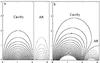 |
Fig. 8 Idealized 2D Cartesian magnetic fields of the cavity and active region a) before and b) after the flare, in a domain 0 < y < π,0 < z < ∞, where z denotes the coronal height. |
Our observational study supports the interpretation that the CME/flare activities in the active region had a causal relationship with the nearby tornado. Clearly, the tornado was dynamically associated with the expansion of the prominence’s helical field and its cavity. It is an open question whether the Hudson effect drove the cavity expansion and the helical field was responding dynamically to the expansion, or if the helical field lost its meta-stability as the result of hydromagnetic disturbances from the CME/flares from the active region. This physical question is worthy of an MHD time-dependent simulation. Evidence of the Hudson effect has been reported in recent solar observational studies (e.g. Sun et al. 2012; Liu et al. 2009). Our study shows the importance of this effect in relation to CMEs, flares, and prominences, and provides observational motivation for theoretical MHD modeling to address the specific questions posed by this relationship.
Online material
Movie of Fig.5 Access here
Movie a of Fig.6 Access here
Movie b of Fig.6 Access here
Acknowledgments
We are obliged to the SDO/AIA, STEREO/EUVI and SWAP teams. N.K.P. acknowledges the facilities provided by the MPS. We are thankful to Joan Burkepile, Thomas Berger, and Wei Liu for their useful inputs. The National Center for Atmospheric Research is sponsored by the US National Science Foundation.
References
- Attie, R., Innes, D. E., & Potts, H. E. 2009, A&A, 493, L13 [NASA ADS] [CrossRef] [EDP Sciences] [Google Scholar]
- Berger, T. E., Shine, R. A., Slater, G. L., et al. 2008, ApJ, 676, L89 [Google Scholar]
- Berger, T., Testa, P., Hillier, A., et al. 2011, Nature, 472, 197 [NASA ADS] [CrossRef] [PubMed] [Google Scholar]
- Gibson, S. E., Foster, D., Burkepile, J., de Toma, G., & Stanger, A. 2006, ApJ, 641, 590 [NASA ADS] [CrossRef] [Google Scholar]
- Gibson, S. E., Kucera, T. A., Rastawicki, D., et al. 2010, ApJ, 724, 1133 [NASA ADS] [CrossRef] [Google Scholar]
- Habbal, S. R., Druckmüller, M., Morgan, H., et al. 2010, ApJ, 719, 1362 [NASA ADS] [CrossRef] [Google Scholar]
- Halain, J.-P., Berghmans, D., Defise, J.-M., et al. 2010, in SPIE Conf. Ser., 7732 [Google Scholar]
- Howard, R. A., Moses, J. D., Vourlidas, A., et al. 2008, Space Sci. Rev., 136, 67 [NASA ADS] [CrossRef] [Google Scholar]
- Hudson, H. S. 2000, ApJ, 531, L75 [NASA ADS] [CrossRef] [PubMed] [Google Scholar]
- Hudson, H. S., Acton, L. W., Harvey, K. L., & McKenzie, D. E. 1999, ApJ, 513, L83 [NASA ADS] [CrossRef] [Google Scholar]
- Janse, Å. M., & Low, B. C. 2007, A&A, 472, 957 [NASA ADS] [CrossRef] [EDP Sciences] [Google Scholar]
- Lemen, J. R., Title, A. M., Akin, D. J., et al. 2012, Sol. Phys., 275, 17 [NASA ADS] [CrossRef] [Google Scholar]
- Li, X., Morgan, H., Leonard, D., & Jeska, L. 2012, ApJ, 752, L22 [NASA ADS] [CrossRef] [EDP Sciences] [Google Scholar]
- Liggett, M., & Zirin, H. 1984, Sol. Phys., 91, 259 [NASA ADS] [CrossRef] [Google Scholar]
- Liu, R., Wang, H., & Alexander, D. 2009, ApJ, 696, 121 [NASA ADS] [CrossRef] [Google Scholar]
- Liu, J., Zhou, Z., Wang, Y., et al. 2012a, ApJ, 758, L26 [NASA ADS] [CrossRef] [Google Scholar]
- Liu, W., Ofman, L., Nitta, N. V., et al. 2012b, ApJ, 753, 52 [NASA ADS] [CrossRef] [Google Scholar]
- Low, B. C., Berger, T., Casini, R., & Liu, W. 2012a, ApJ, 755, 34 [NASA ADS] [CrossRef] [Google Scholar]
- Low, B. C., Liu, W., Berger, T., & Casini, R. 2012b, ApJ, 757, 21 [Google Scholar]
- Mackay, D. H., Karpen, J. T., Ballester, J. L., Schmieder, B., & Aulanier, G. 2010, Space Sci. Rev., 151, 333 [NASA ADS] [CrossRef] [Google Scholar]
- Martin, S. F. 1998, Sol. Phys., 182, 107 [NASA ADS] [CrossRef] [Google Scholar]
- Pettit, E. 1943, ApJ, 98, 6 [NASA ADS] [CrossRef] [Google Scholar]
- Régnier, S., Walsh, R. W., & Alexander, C. E. 2011, A&A, 533, L1 [NASA ADS] [CrossRef] [EDP Sciences] [Google Scholar]
- Su, Y., Wang, T., Veronig, A., Temmer, M., & Gan, W. 2012, ApJ, 756, L41 [NASA ADS] [CrossRef] [Google Scholar]
- Sun, X., Hoeksema, J. T., Liu, Y., et al. 2012, ApJ, 748, 77 [NASA ADS] [CrossRef] [Google Scholar]
- Tandberg-Hanssen, E. 1995, Astrophys. Space Sci. Lib. 199, The nature of solar prominences [Google Scholar]
- Thompson, W. T. 2009, Icarus, 200, 351 [NASA ADS] [CrossRef] [Google Scholar]
- van Ballegooijen, A. A., & Cranmer, S. R. 2010, ApJ, 711, 164 [NASA ADS] [CrossRef] [Google Scholar]
- Wedemeyer-Böhm, S., Scullion, E., Steiner, O., et al. 2012, Nature, 486, 505 [NASA ADS] [CrossRef] [PubMed] [Google Scholar]
- Zhang, M., & Low, B. C. 2003, ApJ, 584, 479 [NASA ADS] [CrossRef] [Google Scholar]
- Zhang, M., & Low, B. C. 2005, ARA&A, 43, 103 [Google Scholar]
Appendix A: Mathematical illustration of the Hudson effect
We give the mathematical solutions for 2D magnetic fields in Fig. 8, which are straightforward to construct by standard techniques. Use
the representation ![\appendix \setcounter{section}{1} \begin{equation} \label{B} \vec{B} = \left[ Q, {\partial A \over \partial z}, -{\partial A \over \partial y} \right] \end{equation}](/articles/aa/full_html/2013/01/aa20503-12/aa20503-12-eq22.png) (A.1)in
terms of the scalar flux-function A(y,z) and the
component
Bx = Q(y,z)
corresponding to the ignorable coordinate x. The initial field
Binitial in Fig. 8a is given by A = Ainitial
and Q = Qinitial, where
(A.1)in
terms of the scalar flux-function A(y,z) and the
component
Bx = Q(y,z)
corresponding to the ignorable coordinate x. The initial field
Binitial in Fig. 8a is given by A = Ainitial
and Q = Qinitial, where
 \arraycolsep1.75ptThe
end-state field Bend has potential field
everywhere with A = Aend, where
\arraycolsep1.75ptThe
end-state field Bend has potential field
everywhere with A = Aend, where
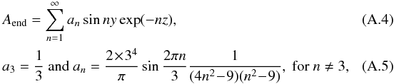 with
Q ≡ 0. Both Binitial and
Bend have the same distribution of normal
field component along the boundary of the domain
0 < y < π,
0 < z < ∞.
with
Q ≡ 0. Both Binitial and
Bend have the same distribution of normal
field component along the boundary of the domain
0 < y < π,
0 < z < ∞.
All Figures
|
Fig. 1 Region around the tornado on 25 September 2011: a) EUVI-A 195 Å; b) AIA 171 Å images. On the EUVI image, the black dashed line shows the position of the AIA limb, and the long diagonal arrow is the epipolar line for the prominence position marked with + on the AIA image. The orange dashed line outlines the position of the southern edge of the active region (AR) corona. |
| In the text | |
|
Fig. 2 EUVI-A 195 Å running-ratio images showing the onset of the three flares (a), b), and c)) and their associated EUV waves (d), e), and f)). In a) the epipolar line shown in Fig. 1a is drawn as a long white arrow, and the solar limb is drawn as a dashed white line. The small white arrow in all images points to the tornado site. The dot-dashed/dashed lines in b) mark the positions of time series shown in Fig. 4, and the orange dashed line along the EUV wave front in e) is the position of the time series in Fig. 3. |
| In the text | |
|
Fig. 3 EUVI 195 Å running-ratio space-time image along the dashed line in Fig. 2e. The three flares are labelled F1, F2, and F3. The red arrow points to the filament. |
| In the text | |
|
Fig. 4 EUVI 195 Å running-difference time-series along a) the vertical and b) the horizontal line in Fig. 2b. The red dashed lines are drawn at the times of flare F1, F2, and F3. In b) the yellow arrows point to the changes in filament structure after the flares. |
| In the text | |
|
Fig. 5 SWAP 174 Å intensity image from 25 September 2011. The arrows show the positions of the cavity and the active region (AR). This frame is taken from the movie “MOVIE5.mp4”. |
| In the text | |
|
Fig. 6 AIA 171 Å intensity image. The diagonal long arrows show the positions of the time-series images through the prominence/tornado, cavity, active region hot loop (AR loop) and active-region (AR) shown in Fig. 7. This is the frame from the movie “MOVIE6b.mp4”. “MOVIE6a.mp4” shows the evolution of this region at earlier times. |
| In the text | |
|
Fig. 7 AIA 171 Å intensity time-series along the diagonal arrows in Fig. 6: a) oscillations of the prominence stem triggered by F1 taken along the bottom white arrow; b) activity triggered by F2 and F3 taken along the middle white arrow; c) tornado activity and cavity changes triggered by F2 and F3 taken along the top arrow. The arrow at the time of the flare (~09.40 UT) points to the movement of the cavity boundary. |
| In the text | |
|
Fig. 8 Idealized 2D Cartesian magnetic fields of the cavity and active region a) before and b) after the flare, in a domain 0 < y < π,0 < z < ∞, where z denotes the coronal height. |
| In the text | |
Current usage metrics show cumulative count of Article Views (full-text article views including HTML views, PDF and ePub downloads, according to the available data) and Abstracts Views on Vision4Press platform.
Data correspond to usage on the plateform after 2015. The current usage metrics is available 48-96 hours after online publication and is updated daily on week days.
Initial download of the metrics may take a while.