| Issue |
A&A
Volume 549, January 2013
|
|
|---|---|---|
| Article Number | A7 | |
| Number of page(s) | 9 | |
| Section | Extragalactic astronomy | |
| DOI | https://doi.org/10.1051/0004-6361/201220439 | |
| Published online | 06 December 2012 | |
Stellar mass versus velocity dispersion as tracers of the lensing signal around bulge-dominated galaxies
1
Leiden Observatory, Leiden University,
Niels Bohrweg 2,
2333 CA
Leiden,
The Netherlands
e-mail: vuitert@strw.leidenuniv.nl
2
Argelander-Institut für Astronomie, Auf dem Hügel 71, 53121
Bonn,
Germany
3
South African Astronomical Observatory,
PO Box 9, 7935
Observatory, South
Africa
4
Department of Astronomy and Astrophysics, University of
Chicago, 5640 S. Ellis
Ave., Chicago,
IL
60637,
USA
5
Department of Astronomy and Astrophysics, University of
Toronto, 50 St. George
Street, Toronto,
Ontario, M5S 3H4, Canada
Received: 25 September 2012
Accepted: 31 October 2012
We present the results of a weak gravitational lensing analysis to determine whether the stellar mass or else the velocity dispersion is more closely related to the amplitude of the lensing signal around galaxies, hence to the projected distribution of dark matter. The lensing signal on smaller scales than the virial radius corresponds most closely to the lensing velocity dispersion in the case of a singular isothermal profile, but is also sensitive on larger scales to the clustering of the haloes. We have selected over 4000 lens galaxies at a redshift z < 0.2 with concentrated (or bulge-dominated) surface brightness profiles from the ~300 square degree overlap between the Red-sequence Cluster Survey 2 (RCS2) and the data release 7 (DR7) of the Sloan Digital Sky Survey (SDSS). We consider both the spectroscopic velocity dispersion and a model velocity dispersion (a combination of the stellar mass, the size, and the Sérsic index of a galaxy). Comparing the model and spectroscopic velocity dispersion we find that they correlate well for galaxies with concentrated brightness profiles. We find that the stellar mass and the spectroscopic velocity dispersion trace the amplitude of the lensing signal on small scales equally well. The model velocity dispersion, however, does significantly worse. A possible explanation is that the halo properties that determine the small-scale lensing signal – mainly the total mass – also depend on the structural parameters of galaxies, such as the effective radius and Sérsic index, but we lack data for a definitive conclusion.
Key words: gravitational lensing: weak / galaxies: halos / galaxies: formation
© ESO, 2012
1. Introduction
Galaxies form and evolve in the gravitational potentials of large dark matter haloes. The physical processes that drive galaxy formation cause correlations between the properties of the galaxies and their dark matter haloes. To gain insight into these processes, therefore, various properties of galaxies (e.g. colour, metallicity, stellar mass, luminosity, velocity dispersion) can be observed and compared (e.g. Smith et al. 2009; Graves et al. 2009). This has lead to the discovery of a large number of empirical scaling laws, such as the Faber-Jackson relation (Faber & Jackson 1976). These scaling laws help us to disentangle the processes that govern galaxy formation, and serve as important constraints for the theoretical and numerical efforts in this field. Although much progress has been made over the past few decades, many details are still unclear and warrant further investigation.
One key parameter in galaxy formation is thought to be the total mass of a galaxy. Galaxies that have more massive dark matter haloes than others attract more baryons as well, consequently forming more stars, which results in higher stellar masses. The relation between the stellar mass and the total mass of galaxies has been studied with observations (e.g. Mandelbaum et al. 2006; van Uitert et al. 2011; Leauthaud et al. 2012; More et al. 2011; Wake et al. 2011), abundance-matching techniques (e.g. Behroozi et al. 2010; Guo et al. 2010; Moster et al. 2010), semi-analytical modelling (e.g. Somerville et al. 2008; Zehavi et al. 2012), and hydrodynamical simulations (e.g. Kereš et al. 2009; Crain et al. 2009; Gabor et al. 2011; Munshi et al. 2012), and the two components have indeed been found to be correlated. Another property of galaxies that is related to the total mass is the velocity dispersion, which is the luminosity-weighted dispersion of the motions of stars along the line-of-sight within a spectroscopic aperture. The velocity dispersion provides a dynamical estimate of the central mass and correlates with the stellar mass (Taylor et al. 2010) and the total mass of galaxies (van Uitert et al. 2011).
A fundamental question that is of interest in this context is which property of galaxies is most tightly correlated to the total mass. This is interesting, because it shows which property in the centre of dark matter haloes is most intimately linked to the large-scale potential, and is therefore least sensitive to galaxy formation processes such as galaxy mergers and supernova activity that introduce scatter in these relations. The properties of galaxies we compare in this work are the stellar mass and the velocity dispersion. There are various other observables that trace the total mass and could have been used instead, but most of them are either expected to exhibit a large amount of scatter (e.g. metallicity), or they are closely related to the stellar mass (e.g. luminosity).
The total mass of galaxies is not directly observable, so can only be determined by indirect means. An excellent tool to do this is weak gravitational lensing. In weak lensing the distortion of the images of faint background galaxies (sources) due to the gravitational potentials of intervening structures (lenses) is measured. From this distortion, the differential surface mass density of the lenses can be deduced, which can be modelled to obtain the total mass. A major advantage of weak lensing is that it does not rely on physically associated tracers of the gravitational potential, making it a particularly useful probe to study dark matter haloes of galaxies that can extend up to hundreds of kpcs, where such tracers are sparse. The major disadvantage of weak lensing is that the lensing signal of individual galaxies is too weak to detect because the induced distortions are typically 10−100 times smaller than the intrinsic ellipticities of galaxies. Therefore, the signal has to be averaged over hundreds or thousands of lenses to decrease the shape noise and yield a statistically significant signal. However, the average total mass for a certain selection of galaxies is still a very useful measurement, which can be compared to simulations.
It is important to note that the lensing signal on small and large scales measures different properties of dark matter haloes. On projected separations larger than a few times the virial radius, the lensing signal is mainly determined by neighbouring structures, so it depends on the clustering properties of the lenses. Within the virial radius, on the other hand, the lensing signal traces the dark matter distribution of the halo that hosts the galaxy and is therefore directly related to the halo mass. In this work, we ignore the lensing signal on large scales and instead focus at the signal on small scales.
This work is a weak-lensing analogy of the analysis presented in Wake et al. (2012), who performed a similar study using galaxy clustering instead of gravitational lensing. One of their main findings is that the spectroscopic velocity dispersion is more tightly correlated to the clustering signal than either the stellar mass or the dynamical mass. This implies that the velocity dispersion traces the properties of the halo that determine its clustering better, i.e. the halo mass or the halo age. As the small-scale weak lensing signal measures the halo mass, it allows us to disentangle the possible explanations of the clustering results.
The outline of this work is as follows. In Sect. 2, we discuss the various steps of the lensing analysis: we start with a description of the lens selection, then provide a brief outline of the creation of the shape measurement catalogues, and finally discuss the lensing analysis. The measurements are shown in Sect. 3, and we conclude in Sect. 4. Throughout the paper we assume a WMAP7 cosmology (Komatsu et al. 2011) with σ8 = 0.8, ΩΛ = 0.73, ΩM = 0.27, Ωb = 0.046, and h70 = H0/70 km s-1 Mpc-1 with H0 the Hubble constant. All distances quoted are in physical (rather than comoving) units unless explicitly stated otherwise.
2. Lensing analysis
In this study we have used the ~300 square degrees of overlapping area between the Sloan Digital Sky Survey (SDSS; York et al. 2000) and the Red-sequence Cluster Survey 2 (RCS2; Gilbank et al. 2011). We used the SDSS to obtain the properties of the lenses (e.g. stellar mass, velocity dispersion), information that is not available in the RCS2. The lensing analysis was performed on the RCS2, because it is about two magnitudes deeper than the SDSS in r′. The increase in depth combined with a median seeing of 0.7′′, which is a factor of two smaller than the seeing in the SDSS, results in a source galaxy number density that is about five times higher, and a source redshift distribution that peaks at z ~ 0.7. Therefore, the RCS2 enables a high-quality detection of the lensing signal, even for a moderate number of lens galaxies.
2.1. Lenses
The SDSS has imaged roughly a quarter of the entire sky, and has measured the spectra for about one million galaxies (Eisenstein et al. 2001; Strauss et al. 2002). The combination of spectroscopic coverage and photometry in five optical bands (u,g,r,i,z) in the SDSS provides a wealth of galaxy information that is not available from the RCS2. To use this information, but also benefit from the improved lensing quality of the RCS2, we used the 300 square degrees overlap between the surveys for our analysis. We matched the RCS2 catalogues to the DR7 (Abazajian et al. 2009) spectroscopic catalogue, to the MPA-JHU DR71 stellar mass catalogue, and to the NYU Value Added Galaxy Catalogue (NYU-VAGC)2 (Blanton et al. 2005; Adelman-McCarthy et al. 2008; Padmanabhan et al. 2008), which yields the spectroscopic redshifts, velocity dispersions, and the stellar masses of 1.7 × 10⁴ galaxies. From these galaxies we selected our lenses using criteria that are detailed below.
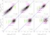 |
Fig. 1 Comparison of the spectroscopic velocity dispersions to the model velocity dispersions for all galaxies with SDSS spectroscopy. The green triangles show the average spectroscopic velocity dispersion for bins of model velocity dispersion, the purple diamonds show the average model velocity dispersion for bins of spectroscopic velocity dispersion. The error bars indicate the scatter. The blue line shows the one-to-one correspondence. Only galaxies with a spectroscopic velocity dispersion error smaller than 15% have been used in the comparison. The velocity dispersions correlate well at z < 0.2, but at z > 0.2 the range in velocity dispersion becomes too narrow to assess whether this is still the case. The square of the correlation coefficient r2 of the galaxies in the range 1.8 < log 10(σmod/spec) < 2.8 km s-1 is shown in the lower right corner of each panel. |
The spectroscopic fibre within which the velocity dispersion is measured has a fixed
size. The physical region where the velocity dispersion is averaged is therefore different
for a sample of galaxies with different sizes and redshifts. To account for this, we
followed Bezanson et al. (2011) and scaled the
observed spectroscopic velocity dispersion to a fixed size of
Re/8 using
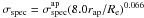 , with
rap = 1.5′′ the radius of the SDSS spectroscopic
fiber, Re the effective radius in the r-band,
and
, with
rap = 1.5′′ the radius of the SDSS spectroscopic
fiber, Re the effective radius in the r-band,
and  the observed velocity dispersion. This
correction is based on the best-fit relation determined using 40 galaxies in the SAURON
sample (Cappellari et al. 2006). However, the
spectroscopic velocity dispersions provided in the DR7 spectroscopic catalogues are
generally noisy for late-type galaxies. To obtain more robust velocity dispersion
estimates for these galaxies, we also predict the velocity dispersion based on quantities
that are better determined following Bezanson et al.
(2011):
the observed velocity dispersion. This
correction is based on the best-fit relation determined using 40 galaxies in the SAURON
sample (Cappellari et al. 2006). However, the
spectroscopic velocity dispersions provided in the DR7 spectroscopic catalogues are
generally noisy for late-type galaxies. To obtain more robust velocity dispersion
estimates for these galaxies, we also predict the velocity dispersion based on quantities
that are better determined following Bezanson et al.
(2011): 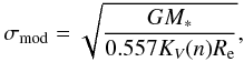 (1)with M∗ the
stellar mass, n the Sérsic index, and
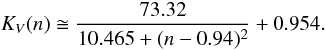
KV(n) a term that
includes the effects of structure on stellar dynamics, and can be approximated by (Bertin et al. 2002)
(1)with M∗ the
stellar mass, n the Sérsic index, and
KV(n) a term that
includes the effects of structure on stellar dynamics, and can be approximated by (Bertin et al. 2002)
 (2)The equation for
σmod is based on the results of Taylor et al. (2010), who demonstrate that the structure-corrected
dynamical mass is linearly related to the stellar mass for a selection of low-redshift
galaxies in the SDSS.
(2)The equation for
σmod is based on the results of Taylor et al. (2010), who demonstrate that the structure-corrected
dynamical mass is linearly related to the stellar mass for a selection of low-redshift
galaxies in the SDSS.
The stellar mass estimates in the MPA-JHU DR7 catalogues are based on the model magnitudes. The Sérsic index and the effective radius in Eq. (1), however, correspond to a different flux, i.e. the Sérsic model flux, which is the total flux of the best fit Sérsic model. This flux is also provided in the NYU-VAGC catalogue, and it differs slightly from the model flux. To calculate σmod consistently, we therefore scaled the stellar mass with the ratio of the model flux to the Sérsic model flux.
Bezanson et al. (2011) find that the model and the observed velocity dispersion correlate very well in the range 60 km s-1 < σ < 300 km s-1, for galaxies in the redshift range 0.05 < z < 0.07, and for a few galaxies with redshifts 1 < z < 2.5. The SDSS spectroscopic sample extends to z ~ 0.5, and therefore contains many more massive galaxies. To determine whether the velocity dispersions correlate well in this range too, we compared the dispersions for the complete SDSS spectroscopic sample in Fig. 1. We find that the velocity dispersions agree well, though at z > 0.2 the range in velocity dispersion becomes too narrow to assess whether the velocity dispersions are still correlated. This is reflected by the correlation coefficient of the log of the velocity dispersions of galaxies in the range 1.8 < log 10(σmod/spec) < 2.8 km s-1, which we show in the corresponding panels.
To study whether the spectroscopic velocity dispersion and the model velocity dispersion
agree equally well for different galaxy types, we split the galaxies based on their
frac_dev parameter from the SDSS photometric catalogues. This parameter
is determined by simultaneously fitting  times the best-fitting De Vaucouleur
profile plus (1-) times the best-fitting exponential
profile to an object’s brightness profile. The frac_dev parameter is
therefore a measure of the slope (or concentration) of the brightness profile of a galaxy.
In the following we refer to lenses with frac_dev >
0.5 as galaxies with a surface brightness profile with a high concentration; these are
bulge-dominated, which is typical of early-type galaxies. The lenses with frac_dev
< 0.5 are referred to as those with a low-concentration
brightness profile; they are disk-dominated as is generally the case for late-type
galaxies. We selected all galaxies with redshifts
z < 0.2, and show the comparison in Fig. 2. We find that for the galaxies with high-concentration
(bulge-dominated) brightness profiles, the spectroscopic and model velocity dispersion
agree very well. For those with low-concentration brightness profiles, however, we find
that the spectroscopic velocity dispersion is ~0.1 dex higher than the model velocity
dispersion. This is not surprising. Taylor et al.
(2010) find that the relation between the stellar mass and the
structure-corrected dynamical mass has a weak dependence on the Sérsic index; i.e., the
ratio of the stellar mass and the dynamical mass increases with increasing Sérsic index
(see Fig. 14 in Taylor et al. 2010). The offset in the relation between spectroscopic and
model velocity dispersion for galaxies with low-concentration brightness profiles is a
direct consequence. It might be caused by the contribution of the disk velocity of spiral
galaxies to the spectroscopic velocity dispersion. One could in principle apply a
correction that depends on the Sérsic index, but we chose to only use galaxies with
high-concentration brightness profiles, because there are very few lenses with
low-concentration brightness profiles in the velocity dispersion range we are interested
in. As a test we repeated the analysis including all lenses, and find that it did not
affect our conclusions.
times the best-fitting De Vaucouleur
profile plus (1-) times the best-fitting exponential
profile to an object’s brightness profile. The frac_dev parameter is
therefore a measure of the slope (or concentration) of the brightness profile of a galaxy.
In the following we refer to lenses with frac_dev >
0.5 as galaxies with a surface brightness profile with a high concentration; these are
bulge-dominated, which is typical of early-type galaxies. The lenses with frac_dev
< 0.5 are referred to as those with a low-concentration
brightness profile; they are disk-dominated as is generally the case for late-type
galaxies. We selected all galaxies with redshifts
z < 0.2, and show the comparison in Fig. 2. We find that for the galaxies with high-concentration
(bulge-dominated) brightness profiles, the spectroscopic and model velocity dispersion
agree very well. For those with low-concentration brightness profiles, however, we find
that the spectroscopic velocity dispersion is ~0.1 dex higher than the model velocity
dispersion. This is not surprising. Taylor et al.
(2010) find that the relation between the stellar mass and the
structure-corrected dynamical mass has a weak dependence on the Sérsic index; i.e., the
ratio of the stellar mass and the dynamical mass increases with increasing Sérsic index
(see Fig. 14 in Taylor et al. 2010). The offset in the relation between spectroscopic and
model velocity dispersion for galaxies with low-concentration brightness profiles is a
direct consequence. It might be caused by the contribution of the disk velocity of spiral
galaxies to the spectroscopic velocity dispersion. One could in principle apply a
correction that depends on the Sérsic index, but we chose to only use galaxies with
high-concentration brightness profiles, because there are very few lenses with
low-concentration brightness profiles in the velocity dispersion range we are interested
in. As a test we repeated the analysis including all lenses, and find that it did not
affect our conclusions.
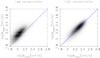 |
Fig. 2 Comparison of the spectroscopic velocity dispersions to the model velocity dispersions for galaxies with low-concentration (frac_dev < 0.5) (left) and with high-concentration brightness profiles (frac_dev > 0.5) (right) in the redshift range 0 < z < 0.2. For the latter, the dispersions agree very well, but for the former, we find that the spectroscopic velocity dispersion is roughly 0.1 dex higher than the model velocity dispersion. |
In Fig. 3, we plot the spectroscopic and model
velocity dispersion as a function of stellar mass. We have only selected galaxies with
redshifts z < 0.2, because at higher redshifts the
range in velocity dispersions is too narrow to establish whether the correlation works
well. We selected all galaxies with high-concentration brightness profiles with a stellar
mass
10.8 < log (M∗) < 11.5
in units of  ; all with a model velocity dispersion
180 km s-1 <
σmod < 300 km s-1; and all
with a spectroscopic velocity
dispersion 180 km s-1 < σspec < 300 km s-1
and a relative error of < 0.15 in σspec.
With these criteria we select 4735, 4218, and 4317 lenses, respectively, and they form the
lens samples of this study.
; all with a model velocity dispersion
180 km s-1 <
σmod < 300 km s-1; and all
with a spectroscopic velocity
dispersion 180 km s-1 < σspec < 300 km s-1
and a relative error of < 0.15 in σspec.
With these criteria we select 4735, 4218, and 4317 lenses, respectively, and they form the
lens samples of this study.
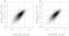 |
Fig. 3 Model velocity dispersion (left) and spectroscopic velocity dispersion (right) as a function of stellar mass. The dashed lines indicate the selection cuts for the lenses. |
2.2. Data reduction
The RCS2 is a nearly 900-square-degree imaging survey in three bands (g′, r′, and z′) carried out with the Canada-France-Hawaii Telescope (CFHT) using the one-square-degree camera MegaCam. The photometric calibration of the RCS2 is described in detail in Gilbank et al. (2011). The magnitudes are calibrated using the colours of the stellar locus and the overlapping Two-Micron All-Sky Survey (2MASS), and they are accurate to < 0.03 mag in each band compared to the SDSS. The creation of the galaxy shape catalogues is described in detail in van Uitert et al. (2011). We refer readers to that paper for more detail, and present here a short summary of the most important steps.
We retrieved the Elixir3 processed images from the Canadian Astronomy Data Centre (CADC) archive4. We used the THELI pipeline (Erben et al. 2005, 2009) to subtract the image backgrounds, to create weight maps that we used in the object detection phase, and to identify satellite and asteroid trails. To detect the objects in the images, we used SExtractor (Bertin & Arnouts 1996). The stars that were used to model the PSF variation across the image were selected using size-magnitude diagrams. All objects larger than 1.2 times the local size of the PSF are identified as galaxies. We measured the shapes of the galaxies with the KSB method (Kaiser et al. 1995; Luppino & Kaiser 1997; Hoekstra et al. 1998), using the implementation described by Hoekstra et al. (1998, 2000). This implementation has been tested on simulated images as part of the Shear Testing Programmes (STEP) 1 and 2 (the “HH” method in Heymans et al. 2006; and Massey et al. 2007, respectively), and these tests have shown that it reliably measures the unconvolved shapes of galaxies for a variety of PSFs. Finally, we corrected the source ellipticities for camera shear, which is an instrumental shear signal that originates in the slight non-linearities in the camera optics. The resulting shape catalogue of the RCS2 contains the ellipticities of 2.2 × 10⁷ galaxies, from which we selected the subset of approximately 1 × 10⁷ galaxies that coincides with the SDSS.
2.3. Lensing measurement
In weak lensing studies, the ellipticities of the source galaxies are used to measure the
azimuthally averaged tangential shear around the lenses as a function of projected
separation: 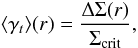 (3)where
  is the difference between the mean projected surface density enclosed by
r and the mean projected surface density at a radius
r, and Σcrit is the critical surface mass density:
is the difference between the mean projected surface density enclosed by
r and the mean projected surface density at a radius
r, and Σcrit is the critical surface mass density:
 (4)with Dl,
Ds, and Dls the angular diameter
distance to the lens, the source, and between the lens and the source, respectively. Since
we lack redshifts for the background galaxies, we selected galaxies with
22 < mr′ < 24
that have a reliable shape estimate (ellipticities smaller than one, no SExtractor flag
raised) as sources. We obtained the approximate source redshift distribution by applying
identical magnitude cuts to the photometric redshift catalogues of the
Canada-France-Hawaii-Telescope Legacy Survey (CFHTLS) “Deep Survey” fields (Ilbert et al. 2006).
(4)with Dl,
Ds, and Dls the angular diameter
distance to the lens, the source, and between the lens and the source, respectively. Since
we lack redshifts for the background galaxies, we selected galaxies with
22 < mr′ < 24
that have a reliable shape estimate (ellipticities smaller than one, no SExtractor flag
raised) as sources. We obtained the approximate source redshift distribution by applying
identical magnitude cuts to the photometric redshift catalogues of the
Canada-France-Hawaii-Telescope Legacy Survey (CFHTLS) “Deep Survey” fields (Ilbert et al. 2006).
To correct the signal for systematic contributions, we computed the shear signal around a large number of random points to which identical image masks were applied, and subtract that from the measured source ellipticities. Details on the calculation of this correction can be found in van Uitert et al. (2011). This correction effectively removes both the impact of residual systematics in the shape measurement catalogues and the impact of image masks on tangential shear measurements. This correction mostly affects large scales (>20 arcmin), since on small scales the lensing signal is generally averaged over many lens-source orientations, causing the systematic contributions to average out. The source galaxy overdensity near the lenses is found to be a few percent at most, confirming that the lenses and sources barely overlap in redshift. Therefore, we do not have to correct the lensing signal for the contamination of physically associated galaxies in the source sample.
Although neither the dark matter nor the baryonic component are described well by a
singular isothermal sphere (SIS), the sum of the two components is remarkably close for
massive elliptical galaxies on scales smaller than the effective radius (e.g. Treu & Koopmans 2004; Koopmans et al. 2009). The SIS signal is given by
 (5)where rE is the
Einstein radius and σlens the lensing velocity dispersion. Van
Uitert et al. (2011) show that for galaxies
with 19.5 < mr′ < 21.5
the SIS profile gives an accurate description of the lensing signal up to
~300−500
(5)where rE is the
Einstein radius and σlens the lensing velocity dispersion. Van
Uitert et al. (2011) show that for galaxies
with 19.5 < mr′ < 21.5
the SIS profile gives an accurate description of the lensing signal up to
~300−500  kpc. Based on the range of stellar masses
and velocity dispersions of our lenses, we expect the majority of our lenses to be central
galaxies (see, e.g. van Uitert et al. 2011; or Mandelbaum et al. 2006, for estimates of
the satellite fraction for galaxies in these ranges) that are considerably more massive
than the average galaxy. The range over which the lensing signal is therefore described
well by an SIS is likely even broader for our lenses.
kpc. Based on the range of stellar masses
and velocity dispersions of our lenses, we expect the majority of our lenses to be central
galaxies (see, e.g. van Uitert et al. 2011; or Mandelbaum et al. 2006, for estimates of
the satellite fraction for galaxies in these ranges) that are considerably more massive
than the average galaxy. The range over which the lensing signal is therefore described
well by an SIS is likely even broader for our lenses.
To determine whether the stellar mass or the velocity dispersion is a better tracer of the amplitude of the lensing signal, we would ideally select lenses in a very narrow range in stellar mass, split those into a high- and a low-velocity dispersion bin, and compare their lensing signals. A difference between the lensing signal of the low- and high-velocity dispersions would indicate a residual dependence on velocity dispersion. Similarly, we would like to select lenses in a very narrow range of velocity dispersion, split them in stellar mass, and compare their signals. Comparing the lensing signals of these four bins would allow us to determine whether the stellar mass or the velocity dispersion is more closely related to the lensing signal on small scales, hence to the projected distribution of dark matter.
Unfortunately, we do not have a sufficient number of lenses for this approach. Instead, we have to select lenses that cover a wider range in stellar mass (and velocity dispersion). We cannot simply split the lenses in velocity dispersion and compare their lensing signals, because the stellar mass and velocity dispersion are correlated, and the high-velocity dispersion bin also has a higher mean stellar mass. To account for this, we determined how the lensing signal scales with stellar mass, and remove this trend from the high and low velocity dispersion bins. We also determined how the lensing signal scales with velocity dispersion, and removed this trend from the high and low stellar mass bins. If the lensing signal of galaxies strongly depends on the velocity dispersion, but only weakly on stellar mass, we expect a clear positive difference between the high and low velocity dispersion bins after we have removed the trend with stellar mass. At the same time, we should only see a very small difference between the high and low stellar mass bin after removing the trend with velocity dispersion. As a result, by studying the differences in the residual lensing signals, we can tell which observable is more closely related to the lensing signal of galaxies.
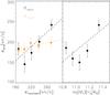 |
Fig. 4 Best-fit lensing velocity dispersion as a function of spectroscopic velocity dispersion (left panel, black), model velocity dispersion (left panel, orange) and stellar mass (right panel). Dashed lines indicate the best-fit linear relation between the observable and σlens. |
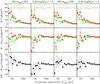 |
Fig. 5 Dependence of the lensing signal on stellar mass and velocity dispersion. In the top row, we show the lensing signal ΔΣ as a function of physical distance from the lens, for the lens samples that have been split by the median value of one of the observables, as indicated in the plots. Red triangles (green diamonds) indicate the signal of the lenses with higher (lower) stellar masses/velocity dispersions. In the middle row, we show the lensing signal of the same samples after we subtracted the trend with the observable that is indicated on top of each column. The difference between the residual trends for the two lens samples are shown in the bottom row. A residual trend indicates that the lensing signal has a residual dependence on the observable indicated inside the corresponding panel of the first row, after removing the dependence on the observable indicated on top of that column. The dotted lines show the best-fit SIS profiles to the difference between the residuals. |
3. Results
To study whether the lensing signal mainly depends on stellar mass or velocity dispersion, we first have to determine how the lensing signal scales with these observables. We discuss how this is done for the model velocity dispersion, and we follow a similar approach for the spectroscopic velocity and the stellar mass. The general procedure is summarized below.
-
We sort the lenses in model velocity dispersion, and divide them into five quintiles.
-
We measure the lensing signal of each quintile, to which we fit an SIS profile on scales between 50
kpc
and 1 Mpc. This is roughly the range where
the galaxy’s dark matter halo dominates the lensing signal. This results in five
best-fit lensing velocity dispersions, σlens. -
We use the five values of σlens to fit the linear relation σlens = amod × (σmod/200 km s-1) + bmod. We show the measurements and the fit in Fig. 4, and give the best-fit parameters in Table 1.
-
We determine the median stellar mass of these lenses, and divide them into a low and high stellar mass sample. We measure the lensing signal of both samples, and show them in the top-left-hand panel of Fig. 5.
-
For each lens in the low and high stellar mass sample, we use the model velocity dispersion to calculate σlens using the linear relation, and subtract their SIS profiles from the lensing signal. The residuals are shown in the middle-left-hand panel of the same figure.
-
Finally, we determine the difference between the residual lensing signal of the high and low stellar mass bins, δ(ΔΣ − ΔΣtrend), which is shown in the bottom-left-hand panel.
When we subtract two SIS profiles with different amplitudes from each other, the result is
also an SIS profile. Therefore, to quantify the residuals, we fit an SIS to
δ(ΔΣ − ΔΣtrend) on the same scales, and determine the residual
Einstein radius,  . These values can be found in Table 2.
Power law parameters.
Similarly, we determine the dependence of the lensing signal on spectroscopic velocity
dispersion and stellar mass. For the spectroscopic velocity dispersion, we fit
σlens = aspec × (σspec/200km s-1) + bspec,
and for the stellar mass, we fit  . The best-fit parameters are shown in
Table 1. These trends are removed from the lensing
signals, and the residuals are shown in Fig. 5 (middle
row).
. The best-fit parameters are shown in
Table 1. These trends are removed from the lensing
signals, and the residuals are shown in Fig. 5 (middle
row).
Residual Einstein radii.
In the bottom panel of the first column of Fig. 5, we
observe that after we have removed the lensing signal dependence on model velocity
dispersion, δ(ΔΣ − ΔΣtrend) is still positive on small scales,
and therefore the lensing signal has a residual dependence on stellar mass. This residual
dependence implies that the lensing signal still depends on stellar mass after removing its
dependence on model velocity dispersion. In the panel next to it, where we have removed the
dependence on stellar mass, we find that the difference between the residuals of the model
velocity samples is consistent with zero, i.e. the lensing signal shows no residual
dependence with model velocity dispersion. These trends are reflected by the values for
in Table 2. The third and fourth columns of Fig. 5
show that if we remove the dependence on spectroscopic velocity dispersion, the difference
in the residual signal of the high and low stellar mass samples is consistent with the
difference between the residual signal of the high and low spectroscopic velocity dispersion
samples after we removed the dependence on stellar mass. Even though the values of the
residual Einstein radii change somewhat if we limit the analysis to smaller scales, which we
expect is mostly due to the larger statistical errors and because we probe different regions
of the haloes, the trends we find do not change qualitatively. A quantitative
characterization of the scale dependence of the signal could be performed with upcoming
lensing surveys.
Since we find that the lensing signal still depends on stellar mass after we remove its dependence on model velocity dispersion, but it does not depend on model velocity dispersion once we have removed the trend with stellar mass, our results suggest that the stellar mass is a better tracer of the lensing signal of galaxies than the model velocity dispersion. Furthermore, the stellar mass and the spectroscopic velocity dispersion trace the lensing signal equally well, because the residual Einstein radii are consistent. As a consistency check, we have also looked at the residual dependence on model velocity dispersion after removing the trend with spectroscopic velocity dispersion, and vice versa. These trends confirm our previous findings: the spectroscopic velocity dispersion is more sensitive to the lensing signal of galaxies than the model velocity dispersion.
There is a weak indication that the lensing signal has a residual dependence on stellar mass after we remove the trend with spectroscopic velocity dispersion, and vice versa. This would imply that both the stellar mass and the velocity dispersion contain independent information on the projected distribution of dark matter around galaxies. Unfortunately, we do not have enough signal-to-noise to obtain a clear detection.
The results depend on the linear relations we have fit to remove the dependence on the
observables. To study how sensitive the residual trends are on these relations, we also fit
them using all galaxies with high-concentration brightness profiles in the
range 100 km s-1 < σspec < 400 km s-1,
100 km s-1 < σmod < 400 km s-1,
and 10.5  , respectively. The best-fit parameters of
these fits are shown in Table 1. We repeated the
analysis using these values, and show the residual Einstein radii between brackets in
Table 2. We find that this does not significantly
change the results, i.e. the model velocity dispersion traces the lensing signal of galaxies
worse than either the stellar mass or the spectroscopic velocity dispersion.
, respectively. The best-fit parameters of
these fits are shown in Table 1. We repeated the
analysis using these values, and show the residual Einstein radii between brackets in
Table 2. We find that this does not significantly
change the results, i.e. the model velocity dispersion traces the lensing signal of galaxies
worse than either the stellar mass or the spectroscopic velocity dispersion.
It is somewhat surprising that σmod is a poorer tracer of the total mass than σspec, particularly because we observe in Fig. 1 that they correlate well. A possible explanation is that they both trace the lensing velocity dispersion equally well on average, but with a different intrinsic scatter. To test this, we draw 106 galaxies from the velocity dispersion function from Sheth et al. (2003), which we adopt as the lensing velocity dispersion σlens. Next we assign them a spectroscopic and model velocity dispersion by drawing from a normal distribution with mean σlens, using a larger scatter for σmod than for σspec. Then we determine the average σlens in the five velocity dispersion bins, as in Fig. 4, and we compare the distribution of σmod and σspec as in Fig. 2. Although we can choose the scatter of σmod and σspec such that we reproduce either Figs. 2 or 4, we cannot find a combination that reproduces both simultaneously. We also tested different distributions for σmod and σspec instead, and found similar results. A difference in intrinsic scatter therefore can at best only partly explain the different performance of σmod and σspec as tracers of the lensing signal.
Another option is that there is another intrinsic property of galaxies with some additional dependence on the lensing signal. To study where the samples differ, we plot the average effective radii and Sérsic indices as a function σmod and σspec in Fig. 6. We find that at low-velocity dispersions, the values of re and n are similar, but at high-velocity dispersions, the lenses in the σspec samples have larger effective radii, whilst the lenses in the σmod have larger Sérsic indices. The difference between the performance of σmod and σspec could therefore be due to an additional dependence of the lensing signal on the structural parameters of the lenses.
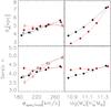 |
Fig. 6 Mean effective radius and Sérsic index as a function of spectroscopic velocity
dispersion (left, black filled diamonds), model velocity dispersion
(left, black open triangles), and stellar mass (right,
black diamonds). In red, we show the averages for the lens samples that
simultaneously satisfy
180 km s-1 < σmod < 300 km s-1,
180 km s-1 < σspec < 300 km s-1,
δσspec/σspec < 0.15
and 10.8 |

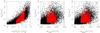 |
Fig. 7 Effective radius as a function of stellar mass (left), model
velocity dispersion (middle), and spectroscopic velocity dispersion
(middle). The black dots show all galaxies with high-concentration
brightness profiles with z < 0.2, the red dots
are the lenses that satisfy
180 km s-1 < σmod < 300 km s-1,
180 km s-1 < σspec < 300 km s-1,
δσspec/σspec < 0.15,
and 10.8 |
To test whether the lensing signal depends on the size of galaxies, we selected the lenses
from the model velocity dispersion sample, and removed the lensing signal dependence
on σmod. We then determined the median effective radius, split
the lenses into a low and high effective radius sample, and measured their residual lensing
signal. As before, we measured the difference between the residual lensing signals of the
high and low effective radius sample, to which we fit an SIS profile. We find
 kpc, which suggests that the lensing signal
depends on the size of a galaxy. However, in Figs. 6
and 7 we find that the effective radius is correlated
with stellar mass, so part of this residual may be caused by the dependence on stellar mass.
Therefore, we repeated the test using the lenses from the stellar mass sample, and removed
the lensing signal dependence on stellar mass. Then we determined the median effective
radius, split the lenses into a low and high effective radius sample, and measured the
difference between their residual lensing signals. We find
kpc, which suggests that the lensing signal
depends on the size of a galaxy. However, in Figs. 6
and 7 we find that the effective radius is correlated
with stellar mass, so part of this residual may be caused by the dependence on stellar mass.
Therefore, we repeated the test using the lenses from the stellar mass sample, and removed
the lensing signal dependence on stellar mass. Then we determined the median effective
radius, split the lenses into a low and high effective radius sample, and measured the
difference between their residual lensing signals. We find
 kpc. Studying the residual dependence on
Sérsic index, we find
kpc. Studying the residual dependence on
Sérsic index, we find  kpc for the model velocity dispersion
sample, and
kpc for the model velocity dispersion
sample, and  kpc for the stellar mass sample. These
results do not provide conclusive evidence that the small-scale lensing signal depends on
these structural parameters.
kpc for the stellar mass sample. These
results do not provide conclusive evidence that the small-scale lensing signal depends on
these structural parameters.
Although the three lens samples overlap, they are not identical. As a result, part of the
trends we observe might actually be due to differences in the lens samples. To test this, we
could define a fourth sample by selecting galaxies that pass all selection criteria, i.e.
180 km s-1 < σmod < 300 km s-1,
180 km s-1 < σspec < 300 km s-1,
δσspec/σspec < 0.15,
and 10.8 
 . However, if we simultaneously select for
stellar mass and model velocity dispersion, we implicitly also select for effective radius
and Sérsic index. This is demonstrated in Figs. 6
and 7, where we show the effective radius and Sérsic
index for the lens samples. When we select lenses that pass all selection criteria, we
exclude lenses with large effective radii and small Sérsic indices at low stellar mass,
lenses with small effective radii and small Sérsic indices at low spectroscopic velocity
dispersions, and lenses with small effective radii and large Sérsic indices at low model
velocity dispersions. If the lensing signal of a galaxy also depends on its structural
parameters, the lensing measurements of this fourth sample could be biased, making the
results harder to interpret.
. However, if we simultaneously select for
stellar mass and model velocity dispersion, we implicitly also select for effective radius
and Sérsic index. This is demonstrated in Figs. 6
and 7, where we show the effective radius and Sérsic
index for the lens samples. When we select lenses that pass all selection criteria, we
exclude lenses with large effective radii and small Sérsic indices at low stellar mass,
lenses with small effective radii and small Sérsic indices at low spectroscopic velocity
dispersions, and lenses with small effective radii and large Sérsic indices at low model
velocity dispersions. If the lensing signal of a galaxy also depends on its structural
parameters, the lensing measurements of this fourth sample could be biased, making the
results harder to interpret.
Wake et al. (2012) find that the ratio of the projected correlation functions of a high and low spectroscopic velocity dispersion sample at a fixed stellar mass is of the order of 1.5−2 on scales < 1 h-1 Mpc, whilst the ratio of a high and low stellar mass sample at a fixed velocity dispersion is close to unity. Our results show, however, that the lensing signal on small scales, which mainly depends on the halo mass, is traced equally well by the stellar mass and the spectroscopic velocity dispersion, and that potential differences are smaller than our statistical errors. The explanation could be that the difference in the amplitudes of the correlation functions is not mainly determined by how well they trace the halo mass. Wake et al. (2012) mention two other possible causes: the relation between the velocity dispersion and halo age is tighter than between stellar mass and halo age, or tidal stripping of satellites that leads to a reduction in stellar mass, but does not affect the velocity dispersion. Although our results favour the latter two explanations, we cannot draw firm conclusions due to the low number of lens galaxies that could be used.
It is important to note that we only study galaxies with high-concentration brightness profiles, whilst the main results of Wake et al. (2012) are based on a sample with mixed galaxy types. Wake et al. (2012) do separate their sample based on colour and on morphology, and find some residual dependence on colour, but not on morphology, which suggests that their results would not have changed by much for a galaxy sample selected with similar criteria as ours here. We note, however, that the range of Sérsic indices of our galaxies is limited, as is shown in Fig. 6. Since Sérsic index and velocity dispersion generally correlate well, it might be that this is diluting the effect in our observations, which then would support the view that the spectroscopic velocity dispersion is a better tracer of the halo mass than the stellar mass. This could be investigated in more detail by repeating this analysis with a larger lens sample.
4. Conclusion
In this work, we study which property of galaxies is most tightly correlated to the weak gravitational lensing signal on small scales for a sample of ~4000 galaxies with high concentration brightness profiles (frac_dev > 0.5) at z < 0.2. The properties we compare are the stellar mass, the spectroscopic velocity dispersion, and the model velocity dispersion. We find that the lensing signal of galaxies is equally well traced by the stellar mass and the spectroscopic velocity dispersion. There is a weak indication of a residual dependence on stellar mass after removing the trend with spectroscopic velocity dispersion, and vice versa. This suggests that both tracers contain independent information on the projected distribution of dark matter around galaxies. Unfortunately, the signal-to-noise of our lensing measurements is not sufficient to make a definite statement.
The model velocity dispersion traces the lensing signal significantly less closely, which is surprising as the spectroscopic velocity dispersion and model velocity dispersion correlate well for our lenses. We find that this cannot be explained solely by assuming a larger intrinsic scatter of the model velocity dispersions compared to the spectroscopic ones. At high-velocity dispersions, however, the lenses in the σmod-sample have smaller effective radii and larger Sérsic indices than those in the σspec-sample. This suggests that these structural parameters contain additional information on the projected distribution of dark matter around galaxies. To test this, we measure how the lensing signal depends on the size and Sérsic index of the lenses. We do not find any conclusive evidence for a residual dependence on these structural parameters, which could be due to insufficient signal-to-noise caused by the relatively small lens sample of this study.
The lensing signal on small projected separations from the lenses mainly depends on the halo mass. Our results therefore suggest that the stellar mass and spectroscopic velocity dispersion trace the halo mass equally well, but the model velocity dispersion does it worse. However, at larger separations, neighbouring structures contribute to the lensing signal as well, and we cannot exclude the possibility that differences between the satellite fractions and large-scale clustering properties of the lens samples also have some effect.
Ideally, one should also remove the potential lensing signal dependence on the structural parameters of galaxies, i.e. split the lens sample both in velocity dispersion and structural parameters, and study the residual dependence on stellar mass. With the current data, we do not have sufficient signal-to-noise to perform such an analysis. However, we expect that at low redshift (z < 0.2), improvement is possible by repeating this analysis on the complete SDSS, while at higher redshifts the overlapping area between the RCS2 and the data release 9 (Ahn et al. 2012) of the SDSS could be used. Ultimately, one could simultaneously fit all these parameters, i.e. Mh = f(σ,M∗,re,n,...), which could also contain products of the parameters such as σM∗, and determine the covariance matrix between the coefficients. The relative magnitude of the coefficients would give new insight into which observables are important, and hence would provide valuable insight into galaxy formation processes. The expected lensing measurements from the space mission Euclid (Laureijs et al. 2011) would be ideal for such a study.
Acknowledgments
We would like to thank Pieter van Dokkum and David Wake for useful discussions, and Peter Schneider for a careful reading of the manuscript. H.H. and EvU acknowledge support from a Marie Curie International Reintegration Grant. HH is also supported by a VIDI grant from the Nederlandse Organisatie voor Wetenschappelijk Onderzoek (NWO). MDG thanks the Research Corporation for support via a Cottrell Scholars Award. The RCS2 project is supported in part by grants to HKCY from the Canada Research Chairs program and the Natural Science and Engineering Research Council of Canada. This work is based on observations obtained with MegaPrime/MegaCam, a joint project of CFHT and CEA/DAPNIA, at the Canada-France-Hawaii Telescope (CFHT) which is operated by the National Research Council (NRC) of Canada, the Institute National des Sciences de l’Univers of the Centre National de la Recherche Scientifique of France, and the University of Hawaii. We used the facilities of the Canadian Astronomy Data Centre operated by the NRC with the support of the Canadian Space Agency.
References
- Abazajian, K. N., Adelman-McCarthy, J. K., Agüeros, M. A., et al. 2009, ApJS, 182, 543 [NASA ADS] [CrossRef] [Google Scholar]
- Adelman-McCarthy, J. K., Agüeros, M. A., Allam, S. S., et al. 2008, ApJS, 175, 297 [NASA ADS] [CrossRef] [Google Scholar]
- Ahn, C. P., Alexandroff, R., Allen de Prieto, C., et al. 2012, ApJS, 203, 21 [NASA ADS] [CrossRef] [Google Scholar]
- Behroozi, P. S., Conroy, C., & Wechsler, R. H. 2010, ApJ, 717, 379 [NASA ADS] [CrossRef] [Google Scholar]
- Bertin, E., & Arnouts, S. 1996, A&AS, 117, 393 [NASA ADS] [CrossRef] [EDP Sciences] [Google Scholar]
- Bertin, G., Ciotti, L., & Del Principe, M. 2002, A&A, 386, 149 [NASA ADS] [CrossRef] [EDP Sciences] [Google Scholar]
- Bezanson, R., van Dokkum, P. G., Franx, M., et al. 2011, ApJ, 737, L31 [NASA ADS] [CrossRef] [Google Scholar]
- Blanton, M. R., Schlegel, D. J., Strauss, M. A., et al. 2005, AJ, 129, 2562 [NASA ADS] [CrossRef] [Google Scholar]
- Cappellari, M., Bacon, R., Bureau, M., et al. 2006, MNRAS, 366, 1126 [NASA ADS] [CrossRef] [Google Scholar]
- Crain, R. A., Theuns, T., Dal la Vecchia, C., et al. 2009, MNRAS, 399, 1773 [NASA ADS] [CrossRef] [Google Scholar]
- Eisenstein, D. J., Annis, J., Gunn, J. E., et al. 2001, AJ, 122, 2267 [NASA ADS] [CrossRef] [Google Scholar]
- Erben, T., Schirmer, M., Dietrich, J. P., et al. 2005, Astron. Nachr., 326, 432 [NASA ADS] [CrossRef] [Google Scholar]
- Erben, T., Hildebrandt, H., Lerchster, M., et al. 2009, A&A, 493, 1197 [NASA ADS] [CrossRef] [EDP Sciences] [Google Scholar]
- Faber, S. M., & Jackson, R. E. 1976, ApJ, 204, 668 [NASA ADS] [CrossRef] [Google Scholar]
- Gabor, J. M., Davé, R., Oppenheimer, B. D., & Finlator, K. 2011, MNRAS, 417, 2676 [NASA ADS] [CrossRef] [Google Scholar]
- Gilbank, D. G., Gladders, M. D., Yee, H. K. C., & Hsieh, B. C. 2011, AJ, 141, 94 [NASA ADS] [CrossRef] [Google Scholar]
- Graves, G. J., Faber, S. M., & Schiavon, R. P. 2009, ApJ, 693, 486 [NASA ADS] [CrossRef] [Google Scholar]
- Guo, Q., White, S., Li, C., & Boylan-Kolchin, M. 2010, MNRAS, 404, 1111 [NASA ADS] [Google Scholar]
- Hoekstra, H., Franx, M., Kuijken, K., & Squires, G. 1998, ApJ, 504, 636 [NASA ADS] [CrossRef] [Google Scholar]
- Hoekstra, H., Franx, M., & Kuijken, K. 2000, ApJ, 532, 88 [NASA ADS] [CrossRef] [Google Scholar]
- Ilbert, O., Arnouts, S., McCracken, H. J., et al. 2006, A&A, 457, 841 [NASA ADS] [CrossRef] [EDP Sciences] [Google Scholar]
- Kaiser, N., Squires, G., & Broadhurst, T. 1995, ApJ, 449, 460 [NASA ADS] [CrossRef] [Google Scholar]
- Kereš, D., Katz, N., Davé, R., Fardal, M., & Weinberg, D. H. 2009, MNRAS, 396, 2332 [NASA ADS] [CrossRef] [Google Scholar]
- Komatsu, E., Smith, K. M., Dunkley, J., et al. 2011, ApJS, 192, 18 [NASA ADS] [CrossRef] [Google Scholar]
- Koopmans, L. V. E., Bolton, A., Treu, T., et al. 2009, ApJ, 703, L51 [NASA ADS] [CrossRef] [Google Scholar]
- Laureijs, R., Amiaux, J., Arduini, S., et al. 2011 [arXiv:1110.3193] [Google Scholar]
- Leauthaud, A., Tinker, J., Bundy, K., et al. 2012, ApJ, 744, 159 [NASA ADS] [CrossRef] [Google Scholar]
- Luppino, G. A., & Kaiser, N. 1997, ApJ, 475, 20 [NASA ADS] [CrossRef] [Google Scholar]
- Mandelbaum, R., Seljak, U., Kauffmann, G., Hirata, C. M., & Brinkmann, J. 2006, MNRAS, 368, 715 [Google Scholar]
- More, S., van den Bosch, F. C., Cacciato, M., et al. 2011, MNRAS, 410, 210 [NASA ADS] [CrossRef] [Google Scholar]
- Moster, B. P., Somerville, R. S., Maulbetsch, C., et al. 2010, ApJ, 710, 903 [NASA ADS] [CrossRef] [Google Scholar]
- Munshi, F., Governato, F., Brooks, A. M., et al. 2012, ApJ, submitted [arXiv:1209.1389] [Google Scholar]
- Padmanabhan, N., Schlegel, D. J., Finkbeiner, D. P., et al. 2008, ApJ, 674, 1217 [NASA ADS] [CrossRef] [MathSciNet] [Google Scholar]
- Sheth, R. K., Bernardi, M., Schechter, P. L., et al. 2003, ApJ, 594, 225 [NASA ADS] [CrossRef] [Google Scholar]
- Smith, R. J., Lucey, J. R., & Hudson, M. J. 2009, MNRAS, 400, 1690 [NASA ADS] [CrossRef] [Google Scholar]
- Somerville, R. S., Hopkins, P. F., Cox, T. J., Robertson, B. E., & Hernquist, L. 2008, MNRAS, 391, 481 [NASA ADS] [CrossRef] [Google Scholar]
- Strauss, M. A., Weinberg, D. H., Lupton, R. H., et al. 2002, AJ, 124, 1810 [NASA ADS] [CrossRef] [Google Scholar]
- Taylor, E. N., Franx, M., Brinchmann, J., van der Wel, A., & van Dokkum, P. G. 2010, ApJ, 722, 1 [NASA ADS] [CrossRef] [Google Scholar]
- Treu, T., & Koopmans, L. V. E. 2004, ApJ, 611, 739 [NASA ADS] [CrossRef] [Google Scholar]
- van Uitert, E., Hoekstra, H., Velander, M., et al. 2011, A&A, 534, A14 [NASA ADS] [CrossRef] [EDP Sciences] [Google Scholar]
- Wake, D. A., Whitaker, K. E., Labbé, I., et al. 2011, ApJ, 728, 46 [NASA ADS] [CrossRef] [Google Scholar]
- Wake, D. A., Franx, M., & van Dokkum, P. G. 2012, ApJ, submitted [arXiv:1201.1913] [Google Scholar]
- York, D. G., Adelman, J., Anderson, Jr., J. E., et al. 2000, AJ, 120, 1579 [Google Scholar]
- Zehavi, I., Patiri, S., & Zheng, Z. 2012, ApJ, 746, 145 [NASA ADS] [CrossRef] [Google Scholar]
All Tables
All Figures
|
Fig. 1 Comparison of the spectroscopic velocity dispersions to the model velocity dispersions for all galaxies with SDSS spectroscopy. The green triangles show the average spectroscopic velocity dispersion for bins of model velocity dispersion, the purple diamonds show the average model velocity dispersion for bins of spectroscopic velocity dispersion. The error bars indicate the scatter. The blue line shows the one-to-one correspondence. Only galaxies with a spectroscopic velocity dispersion error smaller than 15% have been used in the comparison. The velocity dispersions correlate well at z < 0.2, but at z > 0.2 the range in velocity dispersion becomes too narrow to assess whether this is still the case. The square of the correlation coefficient r2 of the galaxies in the range 1.8 < log 10(σmod/spec) < 2.8 km s-1 is shown in the lower right corner of each panel. |
| In the text | |
|
Fig. 2 Comparison of the spectroscopic velocity dispersions to the model velocity dispersions for galaxies with low-concentration (frac_dev < 0.5) (left) and with high-concentration brightness profiles (frac_dev > 0.5) (right) in the redshift range 0 < z < 0.2. For the latter, the dispersions agree very well, but for the former, we find that the spectroscopic velocity dispersion is roughly 0.1 dex higher than the model velocity dispersion. |
| In the text | |
|
Fig. 3 Model velocity dispersion (left) and spectroscopic velocity dispersion (right) as a function of stellar mass. The dashed lines indicate the selection cuts for the lenses. |
| In the text | |
|
Fig. 4 Best-fit lensing velocity dispersion as a function of spectroscopic velocity dispersion (left panel, black), model velocity dispersion (left panel, orange) and stellar mass (right panel). Dashed lines indicate the best-fit linear relation between the observable and σlens. |
| In the text | |
|
Fig. 5 Dependence of the lensing signal on stellar mass and velocity dispersion. In the top row, we show the lensing signal ΔΣ as a function of physical distance from the lens, for the lens samples that have been split by the median value of one of the observables, as indicated in the plots. Red triangles (green diamonds) indicate the signal of the lenses with higher (lower) stellar masses/velocity dispersions. In the middle row, we show the lensing signal of the same samples after we subtracted the trend with the observable that is indicated on top of each column. The difference between the residual trends for the two lens samples are shown in the bottom row. A residual trend indicates that the lensing signal has a residual dependence on the observable indicated inside the corresponding panel of the first row, after removing the dependence on the observable indicated on top of that column. The dotted lines show the best-fit SIS profiles to the difference between the residuals. |
| In the text | |
|
Fig. 6 Mean effective radius and Sérsic index as a function of spectroscopic velocity
dispersion (left, black filled diamonds), model velocity dispersion
(left, black open triangles), and stellar mass (right,
black diamonds). In red, we show the averages for the lens samples that
simultaneously satisfy
180 km s-1 < σmod < 300 km s-1,
180 km s-1 < σspec < 300 km s-1,
δσspec/σspec < 0.15
and 10.8 |
| In the text | |
|
Fig. 7 Effective radius as a function of stellar mass (left), model
velocity dispersion (middle), and spectroscopic velocity dispersion
(middle). The black dots show all galaxies with high-concentration
brightness profiles with z < 0.2, the red dots
are the lenses that satisfy
180 km s-1 < σmod < 300 km s-1,
180 km s-1 < σspec < 300 km s-1,
δσspec/σspec < 0.15,
and 10.8 |
| In the text | |
Current usage metrics show cumulative count of Article Views (full-text article views including HTML views, PDF and ePub downloads, according to the available data) and Abstracts Views on Vision4Press platform.
Data correspond to usage on the plateform after 2015. The current usage metrics is available 48-96 hours after online publication and is updated daily on week days.
Initial download of the metrics may take a while.