| Issue |
A&A
Volume 549, January 2013
|
|
|---|---|---|
| Article Number | A25 | |
| Number of page(s) | 14 | |
| Section | Extragalactic astronomy | |
| DOI | https://doi.org/10.1051/0004-6361/201220070 | |
| Published online | 11 December 2012 | |
The cosmic evolution of oxygen and nitrogen abundances in star-forming galaxies over the past 10 Gyr
1 Institut de Recherche en Astrophysique et Planétologie, CNRS, 14 avenue Édouard Belin, 31400 Toulouse, France
2 IRAP, Université de Toulouse, UPS-OMP, Toulouse, France
3 Instituto de Astrofísica de Andalucía, CSIC, Apartado de correos 3004, 18080 Granada, Spain
e-mail: epm@iaa.es
4 Institute of Astronomy, ETH Zurich, 8093 Zürich, Switzerland
5 Laboratoire d’Astrophysique de Marseille, CNRS-Université d’Aix-Marseille, 38 rue Frédéric Joliot Curie, 13388 Marseille, France
6 European Southern Observatory, Karl-Schwarzschild-Strasse 2, 85748 Garching b. Muenchen, Germany
7 Dipartimento di Astronomia, Università di Padova, vicolo Osservatorio 3, 35122 Padova, Italy
8 INAF – IASF Milano, via Bassini 15, 20133 Milano, Italy
9 INAF – Osservatorio Astronomico di Bologna, via Ranzani 1, 40127 Bologna, Italy
10 Max-Planck-Institut für extraterrestrische Physik, 84571 Garching b. Muenchen, 85748, Germany
11 SUPA Institute for Astronomy, The University of Edinburgh, Royal Observatory, Edinburgh, EH9 3HJ, UK
12 INAF – Osservatorio Astronomico di Trieste, via Tiepolo, 11, 34143 Trieste, Italy
13 INAF – Osservatorio Astronomico di Brera, via Brera, 28, 20159 Milano, Italy
14 MPA – Max Planck Institut für Astrophysik, Karl-Schwarzschild-Str. 1, 85741 Garching, Germany
15 University of Vienna, Department of Astronomy, Tuerkenschanzstrasse 17, 1180 Vienna, Austria
16 Universitá degli Studi dell’Insubria, via Valleggio 11, 22100 Como, Italy
17 Instituto de Astrofísica de Canarias, vía Lactea s/n, 38200 La Laguna, Tenerife, Spain
18 IPMU, Institute for the Physics and Mathematics of the Universe, 5-1-5 Kashiwanoha, 277-8583 Kashiwa, Japan
19 INAF – IASFBO, via P. Gobetti 101, 40129 Bologna, Italy
20 Kapteyn Astronomical Institute, University of Groningen, 9700 AV Groningen, The Netherlands
Received: 20 July 2012
Accepted: 28 September 2012
Aims. The chemical evolution of galaxies on a cosmological timescale is still a matter of debate despite the increasing number of available data provided by spectroscopic surveys of star-forming galaxies at different redshifts. The fundamental relations involving metallicity, such as the mass − metallicity relation (MZR) or the fundamental metallicity relation, give controversial results about the reality of evolution of the chemical content of galaxies at a given stellar mass. In this work we shed some light on this issue using the completeness reached by the 20 k bright sample of the zCOSMOS survey and using for the first time the nitrogen-to-oxygen ratio (N/O) as a tracer of the gas phase chemical evolution of galaxies that is independent of the star formation rate.
Methods. Emission-line galaxies both in the SDSS and 20 k zCOSMOS bright survey were used to study the evolution from the local Universe of the MZR up to a redshift of ~1.32, and the relation between stellar mass and N/O (MNOR) up to a redshift of ~0.42 using the N2S2 parameter. All the physical properties derived from stellar continuum and gas emission-lines, including stellar mass, star formation rates, metallicity and N/O, were calculated in a self-consistent way over the full redshift range.
Results. We confirm the trend to find lower metallicities in galaxies of a given stellar mass in a younger Universe. This trend is even observed when taking possible effects into account that are due to the observed larger median star formation rates for galaxies at higher redshifts. We also find a significant evolution of the MNOR up to z ~ 0.4. Taking the slope of the O/H vs. N/O relation into account for the secondary-nitrogen production regime, the observed evolution of the MNOR is consistent with the trends found for both the MZR and its equivalent relation using new expressions to reduce its dependence on star formation rate.
Key words: galaxies: evolution / galaxies: fundamental parameters / galaxies: abundances / galaxies: starburst
© ESO, 2012
1. Introduction
Chemical abundances provide important clues to the evolutionary history of galaxies along cosmic time since they are the result of the joint action of several physical processes such as supernova feedback, gas inflow/outflow, mergers, and interactions, Even if it is not easy to disentagle the effect of each individual process, it may be possible to constrain galaxy formation theories by studying how chemical abundances for galaxies of different masses and/or in different environments evolve as a function of cosmic epoch. Indeed, as cosmological time progresses, galaxy evolution models predict that both the mean metallicity and stellar mass of galaxies increase with age as galaxies undergo chemical enrichment and grow through merging processes. At any given epoch, the accumulated history of star formation, gas inflows, and outflows, affects a galaxy mass and its metallicity. One therefore expects these quantities to be correlated in some way and this correlation to provide crucial information about the physical processes that govern galaxy formation.
First discovered for dwarf irregular galaxies (Lequeux 1979), the relation between the mass (or luminosity) and the metallicity for different galaxy populations has been the subject of numerous studies (e.g. Skillman et al. 1989; Brodie & Huchra 1991; Zaritsky et al. 1994; Garnett et al. 1997; Pilyugin & Ferrini 2000; Contini et al. 2002). The mass–metallicity relation (hereafter MZR) is now well established in the local universe, thanks to the works of Tremonti et al. (2004) based on SDSS and Lamareille et al. (2004) based on 2dFGRS data, showing that the metallicity of galaxies tends to increase with their mass or luminosity. This trend has been shown to extend to much lower galaxy masses (Lee et al. 2006; Saviane et al. 2008), confirming the idea that a single mechanism may govern galaxy metallicities across five order of magnitude in stellar mass. However, a specific environment and/or high star formation rate (SFR) can explain the observed offset of galaxy population with respect to the global MZR. For instance, nuclear inflows of metal-poor interstellar gas triggered by galaxy interactions can account for the systematically lower central oxygen abundances observed in interacting galaxies (Pérez et al. 2011; Torrey et al. 2012).
Hierarchical galaxy formation models that take the chemical evolution and feedback processes into account are able to reproduce the observed MZR in the local universe (e.g. De Lucia et al. 2004; De Rossi et al. 2007; Finlator & Davé 2007; Davé et al. 2011). However these models rely on free parameters, such as feedback efficiency, which are not yet well constrained by observations. Alternative scenarios proposed to explain the MZR include low star formation efficiency in low-mass galaxies caused by supernova feedback (Brooks et al. 2007) and a variable stellar initial mass function (IMF) that is more top-heavy in galaxies with higher SFRs, thereby producing higher metal yields (Köppen et al. 2007).
The evolution of the MZR on cosmological timescales is now predicted by semi-analytic models of galaxy formation, which include chemical hydrodynamic simulations within the standard Λ-CDM framework (De Lucia et al. 2004; Davè & Oppenheimer 2007; Sakstein et al. 2011). Reliable observational estimates of the MZR of galaxies at different epochs (hence different redshifts) may thus provide important constraints on galaxy evolution scenarios. Estimates of the mass–metallicity – or luminosity–metallicity – relation of galaxies up to z ~ 1.5 have been already derived but have been limited, until recently, to small samples (e.g. Kobulnicky et al. 2003; Liang et al. 2004; Maier et al. 2004, 2005, 2006; Hammer et al. 2005; Savaglio et al. 2005; Lamareille et al. 2006; Liu et al. 2008; Queyrel et al. 2009; Yabe et al. 2012). Recent studies of the MZR (Lamareille et al. 2009; Pérez-Montero et al. 2009; Cowie & Barger 2008; Moustakas et al. 2011; Zahid et al. 2011) have been performed on larger samples ( > 1000 galaxies) thanks to the large and deep spectroscopic surveys (VVDS, DEEP2, GOODS, AGES, etc) devoted to the formation and evolution of galaxies on cosmological timescales. The general observational result of these studies is that the MZR evolves with redshift, in the sense that, on average and for a given stellar mass, high-redshift galaxies are characterised by lower metallicities. Whether the MZR also evolves in terms of shape/slope is still matter of debate. Indeed, Savaglio et al. (2005) conclude that there is a steeper slope in the distant universe, whereas Lamareille et al. (2009) and Pérez-Montero et al. (2009) found flattening of the MZR at redshifts 0.7 < z < 1.0. At higher redshifts Erb et al. (2006) derived a MZR at z ~ 2 lowered by 0.3 dex in metallicity compared with the local estimate, a trend that could extend up to z ~ 3−4 (Maiolino et al. 2008; Mannucci et al. 2009).
However, the redshift evolution of the gas-phase metallicity in galaxies has been questioned recently by Mannucci et al. (2010) and Lara-López et al. (2010). They discovered that metallicity depends not only on the stellar mass, but also on the SFR: for a given stellar mass, galaxies with higher SFR systematically show lower metallicities. This is the so-called fundamental metallicity relation (FMR), i.e., a tight relation between stellar mass, gas-phase metallicity, and SFR. Local SDSS galaxies show very small residuals (~0.05 dex) around this relation (Yates et al. 2012; Brisbin & Harwit 2012). According to Mannucci et al. (2010), the FMR does not evolve with redshift up to z ~ 2.5. This result was later confirmed by Cresci et al. (2012) by studying the zCOSMOS 10k bright sample up to a redshift ≈ 0.8. This would suggest that the observed evolution of the MZR is due to selection effects and to the well-established increase in the average SFR with redshift (Noeske et al. 2007; Elbaz et al. 2007; Daddi et al. 2007).
The study of other indicators of the chemical content of galaxies and their relation with stellar mass and SFR have not been sufficiently explored so far so can shed some light on the issue of the evolution of metallicity with cosmic age. This is the case of the nitrogen-to-oxygen abundance ratio (N/O), which offers some clear advantages over studies of the oxygen abundance alone. On one hand, N is produced mainly by low- and intermediate-mass stars (Henry et al. 2000) in contrast to O, which is produced only by massive stars. This makes N/O a suitable indicator for the chemical evolution of single starbursts (Edmunds & Pagel 1978; Pilyugin et al. 2003). On the other hand, since N is a secondary element (i.e. its yield depends on the previous amount of carbon and oxygen in the stars) for the majority of the metallicity range, its relation with a primary element, such as O, is relatively independent of the chemodynamical effects, such as outflows or inflows (Edmunds 1990; Köppen & Hensler 2005). These effects are the basis of the relation between metallicity and SFR, so the relation between N/O and stellar mass (hereafter MNOR) can be fundamental for studying the chemical evolution of galaxies without worrying about the selection effects of the sampled galaxies at high z. The MNOR for galaxies in the local universe has already been investigated by Pérez-Montero & Contini (2009, hereafter PMC09) who found an increase in N/O with stellar mass, since most of the sampled SDSS galaxies lie in the metallicity range for the production of secondary N. This relation was used by Amorín et al. (2010) to study the chemical evolution of compact galaxies with very high specific SFRs (the green pea galaxies). Later, Thuan et al. (2010) explored the evolution of the relation between stellar mass and N/H up to z = 0.3, exploiting the fact that the production rate of N is faster than for O and its evolution is thus less sensitive to calibration uncertainties.
In this work we investigate both the MZR with its relation to SFR and the MNOR in the Local Universe and their evolutions with cosmic age. This study is based on the SDSS sample for the local universe and the zCOSMOS 20k bright sample for high redshifts (up to a z ≈ 1.32 for the MZR and z ≈ 0.42 for the MNOR).
This paper is organised as follows. In Sect. 2 we describe the SDSS and zCOSMOS samples of the star-forming galaxies used to perform our study of the evolution of both the MZR and the MNOR. The selection of star-forming galaxies and the derivation of physical properties, including stellar mass, SFR, oxygen abundance, and the N/O abundance ratio are described in Sect. 3. In Sect. 4 we give our results and discuss the evolution with cosmic age of the MZR, with a correction to take selection effects due to SFR into account, and of the MNOR. Finally, in Sect. 5 we summarise our work and give our conclusions.
Throughout this paper we normalise the derived stellar masses and the absolute magnitudes with the standard Λ-CDM cosmology, i.e., h = 0.7, Ωm = 0.3 and ΩΛ = 0.7 (Spergel et al. 2003).
2. Sample selection
2.1. The parent SDSS local sample
Ss reference sample for the local universe, we used the Data Release 7 of the Sloan Digital Sky Survey (hereafter SDSS), taking the emission-line measurements from the Max Planck Institute for Astrophysics – Johns Hopkins University (MPA-JHU) catalogue1. The emission-line measurement of this sample is described in Brinchmann et al. (2004). From the whole sample of galaxies, we removed duplicated objects and all those emission-line galaxies whose Hβ, [O ii] λλ 3727, 3729, [O iii] λλ 4959, 5007, Hα, [N ii] λ 6584, and [S ii] λλ 6717,6731 have signal-to-noise ratio (S/N) lower than 2. The choice for this low S/N was motivated by the search for a coincidence between the mass − metallicity relation of the SDSS sample derived in this work and the zCOSMOS subsample at low z, avoiding biases in the sample selection for the derivation of metallicity, as discussed below. The selected sample comprises a total of 299 479 galaxies in the 0.02 < z < 0.20 range, but with a mean value z = 0.068. The lower redshift limit is caused by the lower limit of the spectral coverage of the SDSS sample (3800 Å), which prevents the detection of the [O ii] λ 3727 emission-line at z < 0.02. This lower limit also prevents the sample from being contaminated by nearby objects with an inaccurate determination of their integrated properties due to the limited size of the fibre in the SDSS. as they were not totally covered by the 3′′ fibre of SDSS. All collected emission lines were extinction-corrected using the law by Cardelli et al. (1989) and the reddening constants from the Balmer decrement between Hα and Hβ as compared to the theoretical value for mean nebular conditions given by Storey & Hummer (1995).
2.2. The parent zCOSMOS 20k sample
The COSMOS survey is a large HST-ACS survey, with I-band exposures down to IAB = 28 on a field of ~2 deg2 (Scoville et al. 2007). The COSMOS field has been the object of extensive multiwavelength ground- and space-based observations spanning the entire spectrum: X-ray, UV, optical/NIR, mid-infrared, mm/submillimetre and radio, providing fluxes measured over 30 photometric bands (Hasinger et al. 2007; Taniguchi et al. 2007; Capak et al. 2007; Lilly et al. 2007; Sanders et al. 2007; Bertoldi et al. 2007; Schinnerer et al. 2007; Koekemoer et al. 2007; McCracken et al. 2010).
The main spectroscopic follow-up survey undertaken in the COSMOS field, zCOSMOS (Lilly et al. 2007), used 600 h of ESO observing time with the VIMOS multi-object spectrograph (Le Fèvre et al. 2003) mounted on the Melipal 8m-telescope of the ESO-VLT. The zCOSMOS spectroscopic survey consists of two parts: zCOSMOS-bright and zCOSMOS-deep. The zCOSMOS-deep targets ~10 000 galaxies within the central 1 deg2 of the COSMOS field, selected through colour criteria to have 1.4 ≲ z ≲ 3.0. The zCOSMOS-bright is purely magnitude-limited and covers the whole area of 1.7 deg2 of the COSMOS field. It provides redshifts for ~20 000 galaxies down to IAB ≤ 22.5 as measured from the HST-ACS imaging. The success rate in redshift measurements is very high, 95% in the redshift range 0.5 < z < 0.8, and the velocity accuracy is ~100 km s-1 (Lilly et al. 2009). Each observed object has been assigned a flag according to the reliability of its measured redshift. Classes 3. × , 4. × redshifts, plus Classes 1.5, 2.4, 2.5, 9.3, and 9.5 are considered a secure set, with an overall reliability of 99% (see for details Lilly et al. 2009).
For this work, we used the zCOSMOS-bright survey final release: the so-called 20k sample for about 20 000 galaxies with z ≤ 2 and secure redshifts according to the above flag classification (18 206 objects in total, irrespective of redshift and including stars). Observations for the zCOSMOS-bright survey were acquired with the medium-resolution (R = 600) grism of VIMOS, providing spectra over the 5550–9650 Å wavelength range. The total integration time was set to one hour to secure redshifts with a high success rate. The spectral range of observations enables following important diagnostic emission lines to compute metallicity up to redshift z ~ 1.5. The observations were acquired with a seeing lower that 1.2′′.
2.2.1. Emission-line measurement
Spectroscopic measurements (emission and absorption lines strength) in zCOSMOS were performed through the automated pipeline platefit-vimos (Lamareille et al., in prep.) similar to the one performed on SDSS (e.g. Tremonti et al. 2004) and VVDS spectra (Lamareille et al. 2009). This routine processes spectra in two steps. The stellar component of galaxy spectra is fitted as a combination of 30 single stellar population templates, with different ages and metallicities, from the library of Bruzual & Charlot (2003) resampled to the velocity resolution of zCOSMOS spectra. After removal of the stellar component, emission lines are fitted together as a single nebular spectrum made of a sum of Gaussians at specified wavelengths. Further details can be found in Lamareille et al. (2006, 2009).
For this work we selected those zCOSMOS emission-line galaxies with an S/N higher than two for the involved emission-lines in each redshift regime, which leaves a total of 5331 objects.
3. Physical properties
3.1. Selection of star-forming galaxies
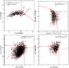 |
Fig. 1 Diagnostic diagrams used to select star-forming objects in the studied sample in each redshift range. From left to right and from up to down: [N ii]/Hα vs. [S ii]/Hα, [N ii]/Hα vs. [O iii]/Hβ, [O ii]/Hβ vs. [O iii]/Hβ, and [O ii]/Hβ vs. [Ne iii]Hβ. |
We selected star-forming galaxies from both the parent SDSS and 20k zCOSMOS samples by means of several empirical diagnostic diagrams based on bright emission-line ratios. We identified narrow-line AGNs (Seyfert 2 and LINERs), taking into account that the broad-line AGNs were already removed. The diagnostic diagrams used for the final classification are not the same for all the galaxies, as the available emission lines depend on the considered redshift range. Indeed, the strategy of the zCOSMOS survey, with a fixed 5550–9650 Å wavelength range, implies that the set of bright emission-lines used in the diagnostic diagrams changes with redshift. This is also true for the oxygen abundance determination, which is based on the same sets of emission lines (see Sect. 3.4).
For the 315 zCOSMOS emission-line galaxies in the redshift range 0.01 < z < 0.13, we used the Hα classification proposed by Lamareille (2007) based on [N ii], [S ii], and Hα emission-line ratios and independent of the reddening. According to this classification, objects are classified as narrow-line AGNs if ![\begin{eqnarray} &&\log\,(\textrm{[\sii]/\ha}) \geq -0.3, \textrm{ and} \nonumber \\[2mm] &&\log\,([\textrm{\nii}]/\textrm{\ha}) > -0.4 \end{eqnarray}](/articles/aa/full_html/2013/01/aa20070-12/aa20070-12-eq42.png) (1)\arraycolsep1.75ptor
(1)\arraycolsep1.75ptor ![\begin{equation} \log\,([\textrm{\nii}/\textrm{\ha}) > -1.05 \cdot \log\,([\textrm{\sii}]/\textrm{\ha}) . \end{equation}](/articles/aa/full_html/2013/01/aa20070-12/aa20070-12-eq43.png) (2)This gives a total of 19 AGNs (6%), which are rejected from the sample to be analysed. The [N ii]/Hα vs. [S ii]/Hα plot for the sample of zCOSMOS 20k emission-line galaxies in this redshift regime is shown in upper left hand panel of Fig. 1.
(2)This gives a total of 19 AGNs (6%), which are rejected from the sample to be analysed. The [N ii]/Hα vs. [S ii]/Hα plot for the sample of zCOSMOS 20k emission-line galaxies in this redshift regime is shown in upper left hand panel of Fig. 1.
For both the redshift range 0.15 < z < 0.44 in the zCOSMOS sample and for the SDSS parent sample, we used the well known and commonly used diagnostic diagrams (e.g. Baldwin et al. 1981; Veilleux & Osterbrock 1987) based on the line ratios [O iii]/Hβ and [S ii]/Hα. In this diagnostic diagram, all points below the separation curve defined by Kewley et al. (2001) can be considered as purely star-forming objects. Since our analysis for both oxygen and nitrogen abundances are based mainly on [N ii] emission-line we preferred not to use the diagram that depends on the [N ii]/Hα for two reasons: i) this diagnostic imposes an upper limit on the N2 = log ([N ii]/Hα) parameter, and hence for the upper metallicity and ii) according to PMC09, both the composite (i.e. a region in the diagram where are objects with a mixture of ionising sources, Kewley et al. 2006) and the AGN region can be contaminated with pure star-forming objects with very high N/O. The total number of zCOSMOS galaxies classified as narrow-line AGN in this redshift range is 188, which is 9.6% of the sample. The right hand upper panel of Fig. 1 shows the sample, along with the curve of separation. The limit log([O iii]/Hβ) = 0.5 shows the separation between Sey2 and LINER galaxies. Regarding SDSS, a total of 44 729 objects were classified as narrow-line AGNs (17.5% of the sample) and 254 750 objects were selected as star-forming galaxies for the analysis of the fundamental relations in the local universe.
At higher redshift (0.47 < z < 0.9), the Hα, [N ii] λ 6584, and [S ii] λλ 6717, 6731 emission lines are not visible anymore in the observed wavelength range of zCOSMOS spectra. In this redshift range, we instead used the blue diagnostic diagrams, as defined by Lamareille et al. (2004), involving the [O iii]/Hβ and [O ii]/Hβ emission-line ratios. Unlike the diagnostic diagrams used for lower redshift, this method does depend on reddening due to the long wavelength baseline between [O ii] λ 3727 Å and Hβ. One way to minimise this dependence is to use the ratio of equivalent widths instead of fluxes as proposed by Kobulnicky et al. (2003), but this method must be corrected owing to the different shape of the underlying stellar continuum in each galaxy. To do so, we took the expression proposed by Liang et al. (2007), who propose the use of a multiplicative factor α to the ratio of equivalent widths of [O ii] and Hβ as a function of the spectral stellar break at 4000 Å. In our case, this break was automatically measured in all the zCOSMOS 20 k spectra at this z by platefit-vimos in the same way as described in Sect. 2.2.1. By considering the separation curve proposed by Marocco et al. (2011), plotted in the left hand lower panel of Fig. 1, we classified 262 galaxies (9.9%) as narrow-line AGNs, and thus we rejected them.
Finally, for the highest redshift galaxies (z > 0.9), we used the method defined by Pérez-Montero et al. (2007) and based on the [O ii] λ 3727 and [Ne iii] λ 3869 emission lines in relation to the brightest available Balmer hydrogen emission line. This diagnostic also utilizes the empirical relation between the emission line fluxes of [O iii] λ 5007 and the [Ne iii] line at a bluer wavelength for a sample of well-characterised ionised gaseous nebulae of the Local Volume. The ratio found by Pérez-Montero et al. (2007) [F([O iii])/F([Ne iii]) ≈ 15.37] agrees within the errors with the ratio measured in those 20k zCOSMOS galaxies with a trustable measurement of the two lines. For those galaxies with no measurement of Hβ, we used Hγ or Hδ and the theoretical relations between Balmer lines from Storey & Hummer (1995) coefficients. We also used this method for those objects in the range 0.5 < z < 0.9 with no confident measurement of the [O iii] emission lines. Regarding extinction correction, unlike the previous redshift range where the ratio of equivalent widths was used, here this does not work due to the stellar continuum variations at [Ne iii] wavelength, according to Pérez-Montero et al. (2007). Instead, we used the Balmer decrement in those galaxies with more than one trustable hydrogen emission-line and, otherwise, we took the derived inner stellar extinction from the spectral synthesis fitting. We also took the separation curve proposed by Marocco et al. (2010), as shown in the lower right-hand panel of Fig. 1. The number of rejected objects in this regime is much higher than in the other three (190, or 46.0% of the sample), but this cannot be taken as a much higher fraction of AGNs in this redshift range. On the contrary, it is probably a selection effect as AGNs have higher S/N for the involved lines than pure star-forming galaxies. In fact, increasing the S/N cut to 3, 5, and 10 increases the fraction of AGNs to 53%, 64%, and 80%, respectively.
Relative number of star-forming galaxies and narrow-line AGNs in each redshift bin in the zCOSMOS bright sample.
3.2. Stellar mass
Total stellar masses for galaxies in the SDSS parent sample were taken from the MPA/JHU catalogue, based on fits to the photometric spectral energy distribution. Regarding masses in the zCOSMOS sample, they were derived from fitting stellar population synthesis models to both the broad-band optical/near-infrared (CFHT: u, i, Ks; Subaru: B, V, g, r, i, z; Capak et al. 2007) and far-infrared (Spitzer/IRAC: 3.6 μm, 4.5 μm; Sanders et al. 2007) photometry, and two spectral features (Hδ absorption line and D(4000) break) when observed in the VIMOS spectra, using a chi-square minimisation for each galaxy. The different methods used to compute stellar masses, based on different assumptions about the population synthesis models and the star formation histories, are described in Bolzonella et al. (2010). The accuracy of the photometric stellar masses is satisfactory overall, with typical dispersions due to statistical uncertainties and degeneracies of the order of 0.2 dex. The addition of secondary bursts to a continuous star formation history produces systematically higher (up to 40%) stellar masses, while population synthesis models taking the TP-AGB stellar phase into account (Maraston 2005; Charlot & Bruzual 2007) systematicaly lower M∗ by 0.10 dex. Finally, the uncertainty on the absolute value of M∗ due to assumptions on the IMF is within a factor of 2 for the typical IMFs usually adopted. In this paper, we have adopted the stellar masses calculated with the stellar population models of Charlot & Bruzual (2007), with the addition of secondary bursts to the standard declining exponantial star formation history.
The left hand panel of Fig. 2 shows the stellar mass distribution (in units of solar mass) of the complete zCOSMOS 20k sample of 18 206 galaxies with secure redshifts. The median value of this distribution is log (M*) = 9.96. The stellar mass distribution for the 4668 star-forming selected galaxies has a median value of 9.66. The lower panel in the same figure shows the redshift distributions for the same samples, with mean values of 0.59 for the complete sample and 0.52 for the selected star-forming galaxies.
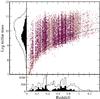 |
Fig. 2 Relation between redshift and stellar mass (in solar masses) for the complete zCOSMOS 20 K sample (brown points) and star-forming selected galaxies (violet points). The solid lines show the logarithmic fitting to the limiting masses of the star-forming sample for levels 25%, 50%, and 75% of completeness. Lower and left hand panels also show the distributions for both the complete sample (empty histogram) and the star-forming galaxies (filled histogram) of z and M∗, respectively. |
For the analysis of stellar masses, we must consider that the minimum “detected” stellar mass is a function of redshift. We thus defined a minimum mass for each redshift bin, which is the lowest mass at which the mass function can be considered reliable and unaffected by incompleteness on mass-to-light (Ilbert et al. 2004; Pozzetti et al. 2007). To calculate the minimum mass, we first computed the limiting mass, which is the stellar mass that an object would have at the limiting magnitude, following the expression  (3)where
  is the limiting mass in solar masses, M∗ the stellar mass in solar masses, Iobs the observed I-band magnitude, and Isel the I-band magnitude limit for each field, which is equal to 22.5 for the studied zCOSMOS sample. In Fig. 2 we show the stellar masses of the selected star-forming galaxies as a function of redshift in the range 0 < z < 1.4. In the same plot we show the logarithmic fits to the 25, 50, and 75 percentile level of the distribution of limiting masses. These fits can be taken as estimates of the minimum masses. In Table 2 we list the values of these fits for different redshift bins and they will be considered in the following as miminum masses for different levels of completeness.
Derived minimum masses (in log(M/M⊙)) for different redshift bins obtained for different levels of completeness.
3.3. Star formation rates
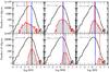 |
Fig. 3 Distribution of the calculated SFR for the star-forming galaxies of the SDSS (in black) and for zCOSMOS star-forming galaxies in different redshift bins (in red). The vertical lines show the medians for the whole zCOSMOS sample (in blue) and for each redshift range (in red). |
For the parent SDSS sample, SFRs were taken from the MPA/JHU catalogue. These SFRs were derived using the technique described in Brinchmann et al. (2004). For the selected star-forming galaxies of the zCOSMOS sample, SFRs were calculated using the luminosity of the brightest available Balmer emission line. These values were corrected for aperture effects using the factors derived from HST photometry. In those cases in which this value was not available, we used Subaru photometry. Extinction correction was carried out using the Balmer decrement for those objects with more than one Balmer hydrogen recombination line with good S/N, and assuming the theoretical ratios at standard conditions of temperature and density from Storey & Hummer (1995) and the Cardelli et al. (1989) extinction law. For objects with only one available Balmer line (a 36% of the selected sample), we assumed a reddening coefficient from the E(B − V) parameter derived from the stellar synthesis fitting. The discrepancies found in those objects with both sources of information about the inner extincion do not vary the SFR distribution significantly. However, it must be stressed that extinction of the gas and stars do not have to correlate, as is the case in this sample, so we preferred to use gas extinction whenever possible.
We derived a linear relation between Hα luminosity and the log(SFR) calculated by Brinchmann et al. (2004) for the DR7-SDSS sample in the Local Volume. This relation yields  (4)and then we derived SFRs in the star-forming selected zCOSMOS galaxies. In those redshift ranges (i.e. for z > 0.44) for which Hα is not observed in the VIMOS spectra, we used Hβ, Hγ, or Hδ emission lines instead, based on the theoretical coefficients between Balmer hydrogen lines from Storey & Hummer (1995) for typical values of both electron temperature and density.
In Fig. 3 we compare the SFR distribution of the SDSS galaxies with the corresponding SFR distributions for different redshift bins in the zCOSMOS selected sample. The vertical blue solid line shows the median SFR for the whole zCOSMOS sample (0.75 M⊙/yr), while the red vertical solid line shows the median SFR for each plotted bin. As can be observed, on one hand the median value for the whole zCOSMOS sample is higher than for the SDSS (with a median of 0.25 M⊙/yr) and the median SFR in each bin increases with z from a value log(SFR) = −0.41 M⊙/yr in the range 0 < z < 0.2 up to log(SFR) = 1.93 M⊙/yr for z > 1.0. This increase in SFR with cosmic time has already been established well by several authors (e.g. Daddi et al. 2007; Bouché et al. 2010), but may be also a selection effect when observing the brightest galaxies at larger z.
3.4. Metallicity
The metallicity of the studied star-forming galaxies can be estimated using the oxygen abundances of their gas phase as a proxy. The most accurate method of deriving this chemical abundance is based on the previous determination of the electron temperature of the gas, via the intensity ratio of nebular-to-auroral emission lines (e.g. [O iii] λλ 5007, 4363) and the relative intensity of the strongest nebular emission lines to a hydrogen recombination line (the so-called Te-method). However, as no information is available in the VIMOS spectra of the zCOSMOS 20 k sample about the weak auroral lines, it is necessary to apply strong-line methods. These are based on direct calibration of the relative intensity of the strongest collisionally excited emission lines with grids of photoionisation models or samples of objects with an accurate determination of the oxygen abundance.
In this work, our aim is to derive metallicities that agree with those derived using the Te-method. Therefore, for the SDSS sample and the zCOSMOS galaxies in the redshift range 0.01 < z < 0.44, we used the calibration of the N2 parameter proposed by PMC09, which is based on a sample of objects with a good determination of 12 + log (O/H) via the Te-method. The N2 parameter, defined as the ratio of [N ii] λ 6584 to Hα by Storchi-Bergmann et al. (1994), has been already used by Denicoló et al. (2000) as a metallicity proxy. The main advantages of this parameter are i) its independence on reddening and flux calibration and ii) its monotonical relation with Z over a very wide range of metallicity. The PMC09 calibration, as discussed in Queyrel et al. (2012), is also consistent with other calibrations of the N2 parameter based on photoionisation models (e.g. Denicoló et al. 2002; Pettini & Pagel 2004; Nagao et al. 2006). According to Pérez-Montero & Díaz (2005), the main drawbacks of this parameter are its dependence on the ionisation parameter, the equivalent effective temperature, and the N/O. Taking all these effects into account, the N2 parameter presents an overall uncertainty of about 0.3 dex across the entire metallicity range. This makes this parameter to be very uncertain for the determination of chemical abundances in single objects, but it offers many advantages when it is used with statistical purposes.
For higher redshifts, as the [N ii] emission-line is not accessible anymore in VIMOS spectra, we derived metallicities using the R23 parameter. This was defined by Pagel et al. (1979) as the relative sum of [O ii] λ 3727 and [O iii] λλ 4959, 5007 to Hβ intensities. Its relation with Z is bivaluated (i.e. it increases with increasing Z at low Z and it decreases with increasing Z at high Z) and it has a strong additional dependence on ionisation parameter and equivalent effective temperature. To minimise this dependence we used the calibration proposed by Kobulnicky et al. (2003) based on the photoionisation models from McGaugh (1991). This calibration takes into account the dependence of R23 on the ionisation parameter with additional terms as a function of the [O ii]/[O iii] ratio. The choice of the calibration branch (low- or high-Z) for each object was done according to the value providing less dispersion in the resulting mass − metallicity relation. Using this criterion, we selected the upper-branch calibration in all cases translating into oxygen abundances with a lower limit of 12 + log (O/H) = 8.0. However, it is expected that a subsample of the objects have lower metallicities, as those identified by Maier et al. (in prep.) using ISAAC-VLT near-IR observations of zCOSMOS galaxies of the bright sample and measuring emission-lines which allow the choice of the appropriate branch of the R23 calibration. An estimate of the relative weight of these metal-poor objects in the z bins where double-valued strong-line methods were used can be obtained from the local SDSS sample. The proportion of objects with 12+log(O/H) < 8.0 from the N2 method is only 0.2%, and if we take into account the minimum mass at 50% of completeness for z > 0.5, is only a 0.016%.
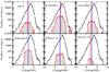 |
Fig. 4 Distribution of the calculated 12+log(O/H) for the star-forming galaxies of the SDSS (black histogram) and zCOSMOS (red histograms) for different redshift bins. The vertical lines show the medians for the whole zCOSMOS sample (in blue) and for each redshift range (in red). |
Regarding the reddening dependence for the [O ii]/Hβ ratio, we used the same procedure based on equivalent widths and the factor α as a function of D(4000), as described in Sect. 3.1.
Finally, for galaxies with a redshift z > 0.9, we used the method described by Pérez-Montero et al. (2007) based on the relation between [Ne iii] λ 3869 and [O iii] λ 5007 (the so-called O2Ne3 parameter) and the theoretical relation between Hβ and other Balmer lines at bluer wavelengths with enough S/N (i.e. Hγ and Hδ). For these objects, we also considered reddening correction from the Balmer decrement when more than a hydrogen emission-line is available and, otherwise, we took the stellar extinction derived from spectral synthesis fitting as described in Sect. 3.1.
As already described by Kewley & Ellison (2008), important differences can arise between the metallicities derived using different strong-line methods and/or different calibrations of the strong emission-line ratios. In our case, as the PMC09 calibration of the N2 parameter is based on the compilation of objects with a “direct” determination of the oxygen abundance, while the calibration of R23 is based on sequences of photoionisation models, this difference can be very large. To convert the metallicities derived from R23 and O2Ne3 parameters to those estimated in the local universe from the N2 parameter, we used the following linear relations which is based on models by Charlot & Longhetti (2001) as described in Lamareille (2007)  (5)for the lower branch calibration of R23 and
  (6)for the calibration of the upper branch.
In Fig. 4 we show the oxygen abundance distribution for the SDSS selected star-forming galaxies compared with the same distributions for different z bins in the zCOSMOS sample in order to investigate their completeness in metallicity. In the lowest redshift bins (z < 0.4), the high-metallicity values measured in SDSS galaxies are not reached in zCOSMOS basically because almost no massive galaxies are detected, as the sampled volume probed by zCOSMOS at these low redshifts is much smaller than for SDSS. For low metallicities, no values lower than 12+log(O/H) < 7.7 are found in zCOSMOS in the same low z bins because the minimum [N ii] flux which can be measured in this survey is brighter than in SDSS. Nonetheless, the statistical weight of this low-metallicity queue in the SDSS sample is negligible (0.02%). We can thus consider that our selection of zCOSMOS galaxies is representative, in terms of metallicity, of the low-redshift (z < 0.4) star-forming galaxies.
At larger redshift (z > 0.4), there is also a selection effect related to the minimum emission-line flux detected in zCOSMOS, but this time it affects the high-metallicity regime. Indeed, in this regime, all oxygen abundances were derived from the upper-branch calibration of R23 (or O2Ne3 for z > 0.9), where weaker relative emission lines imply higher Z. Therefore, the minimum detectable [O ii] and [O iii] emission lines imposes an upper limit on the metallicity of zCOSMOS galaxies. However, as in the case of low-metallicity galaxies at low redshift, this has a negligible impact on the final distributions as SDSS galaxies with 12+log(O/H) > 9 only represents 1.14% of the total sample. Regarding the cutoff seen for lower metallicity at this redshift regime, it corresponds to the choice of the upper branch calibration in all cases (12+log(O/H) > 8.0). Although a number of galaxies is expected to have low metallicities (as those observed with ISAAC in Maier et al., in prep.), these galaxies have a negligible statistical weight when we compare with the SDSS sample (0.2%). In any case, this number cannot be taken as an estimate of the relative number of very-low metallicity galaxies in all the zCOSMOS sample.
3.5. Nitrogen-to-oxygen abundance ratio
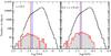 |
Fig. 5 Distribution of the calculated log(N/O) for the star-forming galaxies of the SDSS (black histogram) and zCOSMOS (red histograms) for different redshift bins. The vertical lines show the medians for the whole zCOSMOS sample (in blue) and for each redshift range (in red). |
The N/O was derived for both the SDSS sample and the zCOSMOS 20k sample (up to z ~ 0.42 only), using the empirical calibration of the N2S2 parameter. This parameter is defined as the ratio of the emission-line fluxes of [N ii] λ 6584 and [S ii] λλ 6717, 6731, which according to PMC09 has a linear relation with log(N/O). Although the ratio between [N ii] λ 6584 and [O ii] λ 3727, the so-called N2O2 parameter, is also a good indicator of N/O (Pérez-Montero & Díaz 2005; PMC09), we did not use it for sake of consistency with the zCOSMOS data, for which no [O ii] information exists for z < 0.5.
In Fig. 5 we show the distribution of log(N/O) for both the SDSS and zCOSMOS samples. Two redshift bins are considered for the zCOSMOS sample: z ≤ 0.2 and 0.2 < z ≤ 0.42. Contrary to metallicity, the N/O is well sampled for low values in zCOSMOS using the N2S2 parameter. However, this is not the case for high values of N/O. As in the case of metallicity, this is because only few massive galaxies are sampled at these redshifts within zCOSMOS, and thus very high values of N/O are missing in this sample. This effect is also seen in the zCOSMOS sample because the median log(N/O) for the lower redshift bin (−1.38) is lower than for z larger than 0.2 (−1.29), and both of them are much lower than the median log(N/O) for the entire SDSS sample (−0.83) since more massive galaxies are sampled on it.
4. Results and discussion
4.1. Cosmic evolution of the mass–metallicity relation
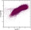 |
Fig. 6 Relation between stellar mass (in units of M⊙) and 12 + log (O/H) for the selected star-forming galaxies of the SDSS-DR7. The red solid line shows the quadratical fit to the medians in bins of 0.2 dex of stellar mass. |
Average offsets between the medians measured in the SDSS reference sample and for the star-forming galaxies of zCOSMOS 20k in each redshift bin for the mass − metallicity relation (MZR), the star formation-corrected mass − metallicity relation (SMZ), and the relation between stellas mass and N/O (MNOR).
To consistently study the cosmic evolution of the MZR we derived its shape in the selected star-forming galaxies of the SDSS, which are representative of the local universe. As described in the sections above we used the compiled stellar masses from the MPA/JHU catalogue and calculated oxygen abundances from the PMC09 calibration of the N2 parameter. The derived MZR for the SDSS is shown in Fig. 6. We computed a quadratical fit to the median values of O/H per stellar mass bins of 0.2 dex. The resulting fit has the following expression  (7)where y is 12 + log (O/H) and x is log (M∗) in units of M⊙. This fit is valid in the range of stellar mass 8.0 < log (M/M⊙) < 11.8. The dispersion was calculated as the standard deviation of the residuals to the resulting fit, giving a result of 0.090 dex. This dispersion is slightly larger for log (M∗) < 10 (0.105 dex) than for higher stellar masses (0.081 dex). We checked that our quadratical fit is consistent with the results given by Kewley & Ellison (2008) for a similar subsample of the SDSS. By converting our oxygen abundances to those studied in that work using different strong-line methods or calibrations of N2, we measured that our median Z is 0.10 dex higher on average for all stellar masses. However, we also found that by increasing the S/N cutoff of our sample to 10, the agreement with the fittings of the MZR provided by Kewley & Ellison (2008) is perfect. Therefore, we conclude that using a high S/N cutoff introduces a selection effect in the subsample, which mainly affects to the metal-rich galaxies when it is applied to all the involved emission lines.
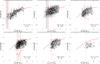 |
Fig. 7 Cosmic evolution of the MZR for six different redshift bins increasing from left to right and from up to down. The red solid line shows the fit to the MZR in the SDSS data. Grey areas show the ± σ intervals to the Z medians fits in different mass bins for each redshift range. The vertical lines show the minimum masses for 25%, 50% and 75% levels of completeness. Red crosses represent low-Z objects in the sample found using ISAAC near-IR observations (Maier et al., in prep.). |
In Fig. 7, we show the MZR for six different redshift bins between 0.01 and 1.32 and compared to the local MZR derived above. Each panel also shows the ± σ curves of the medians of Z in each mass bin and the minimum masses for different levels of completeness as derived in Sect. 3.2. In the three panels correspondinbg to z between 0.4 and 1.0 we show the small subsample of zCOSMOS galaxies observed in the near-infrared (Maier et al., in prep.) and for which oxygen abundances from the lower calibration of the R23 parameter have been derived.
In Table 3, we summarise for each redshift bin the vertical offset between the local MZR and the average of medians for different mass intervals in each z bin. We also give the corresponding dispersions, calculated as the standard deviation of all the medians. In all cases, for the sake of consistency, these offsets were calculated taking from the SDSS those subsamples of objects in the same metallicity and stellar mass range measureable in each z bin of zCOSMOS. The inspection of the values listed in that table leads to the following. (i) The derived median oxygen abundance for the same bins of stellar mass increases with cosmological age so that it was around half the present value at z ≈ 1 ( ≈ 8 Gyr ago). (ii) The increase in the oxygen abundance with cosmic time is not uniform but, on the contrary, it looks to be significantly larger above z ≈ 0.5. (iii) Both the dispersion associated with the derived medians, and the oxygen abundance uncertainties intrinsic to the strong-line methods for each z bin, are larger than the offset for z < 1.0.
Some authors (e.g. Kobulnicky et al. 1999) have warned that taking too low a threshold of S/N for the Balmer emission lines introduces significant uncertainties in the determination of metallicity using strong-line methods, such as R23. On the contrary, as explained in previous sections, taking too high a threshold for certain lines can introduce a bias in the selected sample, To quantify how changing the S/N threshold for Balmer lines affect the median Z in the different redshift bins, we calculated them taking only Balmer emission-lines with S/N > 5, instead of 2. Our results indicate that the number of selected galaxies is considerably decreased for the high z bins (more than 60% for z > 1 and more than 35% for z > 0.4). In Table 3 we also list the Z offsets in relation to the SDSS MZR. All of them give higher Z than in relation to the samples with S/N threshold of two for all the involved emission lines, and this difference increases with z, as an increasing number of low-Z galaxies is excluded in each bin. However, the trend to finding lower median Z with higher z is maintained, although serious caveats must be taken for the intensity of this evolution when selection effects due to different S/N threshold criteria are imposed.
4.2. The SFR-corrected mass–metallicity relation and its evolution
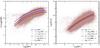 |
Fig. 8 To the left MZR and quadratical fits for different bins of log SFR. To the right, same plot for the relation between log (N/O) and stellar mass. |
Stellar mass and metallicity are two of the main fundamental parameters of galaxies. Their relationship for complete samples of galaxies, as shown in the above section, gives us valuable information about the main mechanisms governing the evolution of galaxies. However, recent works (e.g. Mannucci et al. 2010; Lara-López et al. 2010) have demonstrated the important role of SFR, which is also tightly related to stellar mass and metallicity and thus affects the shape and the dispersion of the MZR. For instance, galaxies with higher SFR have systematically lower metallicities. This effect could be explained by invoking the interaction of galaxies with inflows of unenriched gas that triggers the episodes of star formation and reduces the relative abundance of oxygen in the gas phase. For this reason, Mannucci et al. (2010) defines a FMR that is basically a surface in the three-dimensional space formed by stellar mass, Z, and SFR in which neither selection effects due to SFR appear nor evolution with z are detected up to z ~ 2.5. This lack of evolution in the defined 3D surface (although other authors, such as Lara-López et al. 2010, defined it as a plane) is also found for a subsample of the zCOSMOS-bright galaxies in the redshift range 0.2 < z < 0.8 (Cresci et al. 2012). However, in this paper, since we try to isolate the metallicity evolution with cosmic age independently of the stellar mass, we redefine the question, isolating the dependence of Z with SFR to remove the selection effects at high z. In the left hand panel of Fig. 8, we show the MZR with different quadratical fits for different bins of SFR for the aforementioned selected star-forming galaxies of the SDSS. As mentioned above, there is a trend toward obtaining lower 12+log(O/H) for higher SFRs. We then applied the SFR correction only to the metallicity, in order to remove possible selection effects at higher z. We thus used the SFR-corrected MZR (hereafter SMZ relation).
By inspecting Fig. 8 again, we clearly see that the evolution of the vertical offsets between the quadratical fits to subsamples with different SFRs is not linear. Indeed, we can fit a quadratical SFR-correction to the Z axis in order to reduce the dispersion and remove the dependence on SFR. The additional term to add to the metallicity axis is  (8)In Fig. 9 we show the corrected MZR, in which the corrected metallicity is represented as a function of the stellar mass. The resulting quadratical fit to the Z medians in bins of 0.2 dex in stellar mass in the range 8.0 < log (M/M⊙ < 11.8 is
  (9)where y = 12+log(O/H)+f(SFR) and x is the stellar mass in units of solar masses. The dispersion of this new relation is slightly lower than for the uncorrected MZR (0.083 dex) and, as in the uncorrected case, the dispersion is lower for masses higher than log(M∗) = 10.0 (0.075 dex) than for lower masses (0.097 dex). An explanation of the fact that the dispersion is only reduced by 0.01 dex at all stellar masses can be found the majority of SDSS galaxies not having extreme SFR values. The dispersion in the SFR distribution of the SDSS sample is only 0.37 dex. A much more thorough calculation of this correction should be done using well-known galaxies with extreme values of the SFR to put more precise constraints on the SFR-correction term of the SMZ.
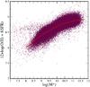 |
Fig. 9 Relation between stellar mass in units of M⊙ and 12+log(O/H) with the correction depending on log(SFR) for the star-forming selected galaxies of the SDSS-DR7. The red solid line shows the quadratical fit to the medians in bins of 0.2 dex of stellar mass. |
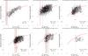 |
Fig. 10 Cosmic evolution of the SFR-corrected MZR for six different redshift bins increasing from left to right and from up to down. The red solid line shows the fitting to the SMZ in the SDSS data. Upper and lower solid lines show the ± σ intervals to the fitting to the y medians in different mass bins for each redshift range. The vertical lines show the minimum mass limits for 25%, 50% and 75% levels of completeness. Red crosses represent low-Z objects in the sample found using ISAAC near-IR observations (Maier et al., in prep.). |
To study to what extent selection effects of the SFR can affect the conclusions reached from the study of the MZR, we applied the SFR-correction to the selected zCOSMOS galaxies at different z bins. The SMZ is plotted in Fig. 10 for the same six different redshift bins between 0.01 and 1.32 with respect to the relation derived for the SDSS sample. The panels also show the ± 1σ bands around the fitting to the medians for Z + f(SFR) in each mass bin and the minimum mass for different levels of completeness. In Table 3, we summarise for each redshift bin the vertical offset between the reference SDSS SMZ and the average of median offsets for each mass bin and the dispersion, calculated as the standard deviation of the residuals to the fitting.
The inspection of the values listed in that table leads to the following conclusions. (i) There is still a trend toward lower median values of the SFR-corrected Z for higher z, although the measured offsets are lower. This implies that, although the MZR is affected by SFR selection effects for samples taken at high z, these are not sufficient to explain the observed evolution, as stated in other studies (e.g. Mannucci et al. 2010; Cresci et al. 2012). (ii) The dispersion of the SFR-corrected Z is not noticeably lower in each z bin than for the MZR, possibly because that the SFR distributions for each z bin do not have very large dispersions, so the correction affects the median value but not the dispersion of each distribution.
4.3. The relation between stellar mass and nitrogen-to-oxygen ratio and its evolution
The N/O complements the study of the chemical composition of the nebular phase of star-forming galaxies, and it is a robust indicator of the chemical evolution of galaxies. Besides, as the production rate of secondary N is faster than for O (Henry et al. 2000; Thuan et al. 2010), the amplitude of the evolution of its relation with stellar mass gives more reliability to the conclusions reached about its evolution with cosmic age.
Although the relation between stellar mass and N/O (hereafter MNOR) has been already studied by PMC09, we re-calculated this relation using the same selected star-forming galaxies of the SDSS in order to be compared with the zCOSMOS galaxies at higher z. In Fig. 11 we show this relation between stellar mass and log(N/O) for the selected star-forming galaxies of the SDSS-DR7. As explained above, the N/O was calculated using the PMC09 calibration of the N2S2 parameter. As in the case of the MZR, there is a trend toward finding higher N/O for more massive galaxies because all galaxies in this sample already lie in the regime of production of secondary N and so its N/O increases with metallicity. We performed a quadratical fit to the medians of N/O in bins of stellar mass of 0.2 dex in the stellar mass range 8.6 < log (M/M⊙) < 11.6 which gives the following expression:  (10)where y is log(N/O) and x is log(M∗) in units of solar masses. The dispersion, calculated as the standard deviation of the residuals, is equal to 0.144 dex. Contrary to the MZR relation, this dispersion is slightly lower for masses greater than 1010 solar masses (0.136 dex) than for lower masses (0.156 dex). The more restricted stellar mass range where the fit is possible and the higher dispersion for lower stellar masses are possibly owing to the presence of objects with additional primary N production at the low stellar mass regime.
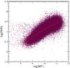 |
Fig. 11 Relation between stellar mass in units of M⊙ and log(N/O) for the star-forming selected galaxies of the SDSS-DR7. The red solid line shows the quadratical fit to the medians in bins of 0.2 dex of stellar mass. |
Besides, unlike the MZR too, there is no apparent selection effect due to different values of the SFR, as can be seen in right hand panel of Fig. 8. This lack of SFR-dependence of the relation between stellar mass and N/O could be a confirmation that the relation between Z and SFR is mainly due to the inflows of metal-poor gas, which would trigger the star formation, decreasing the relative abundance of the metals but which, in contrast, do not affect the ratio between secondary and primary elements (Edmunds 1990).
Therefore, the study of the evolution of the MNOR with cosmic time represents a robust tool for studying the evolution of the chemical content of galaxies as a function of the age of the Universe, as N/O does not depend on selection effects related to SFR. In Fig. 12, we show the evolution of this relation for the two redshift bins in zCOSMOS for which we were able to derive the N/O using the N2S2 parameter. The offsets between the relation derived in the SDSS and for the two analysed z bins and their dispersions are listed in Table 3. The analysis of the obtained values leads to the following conclusions. (i) For a given stellar mass, there is a significant evolution in the median N/O abundance ratio of galaxies from z ~ 0.4 up to now. (ii) This evolution is a consequence of the evolution of the metallicity of galaxies with cosmic age. As can be seen in Fig. 13, the average relation between 12 + log (O/H) and log (N/O) in the regime of production of secondary nitrogen is kept in the two redshift bins. (iii) This evolution cannot be due to any selection effect of the sampled galaxies at high redshift that have, on average, larger SFR, because N/O is not affected by inflows of metal-poor gas in galaxies. (iv) In the secondary nitrogen production regime, N/O increases linearly with oxygen abundance, as can be seen in Fig. 13. Therefore the N/O evolution derived from z ≈ 0.3 can be transformed into metallicity evolution using the slope of this linear relation. This slope is around 1.4 for both the two redshift bins analysed, so this gives a variation in 12+log(O/H) of 0.1 dex on average, which is slightly higher than the values found using both MZR and SMZ. However, it must be taken the large scatter into account in the N/O vs. O/H when computing the O/H evolution in this way.
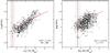 |
Fig. 12 Cosmic evolution of the MNOR for two different redshift bins. The red solid line shows the fit to the MNOR in the SDSS data. Upper and lower solid lines show the ± σ intervals to the fitting to the N/O medians in different mass bins for each redshift range. The vertical lines show the minimum mass limits for 25%, 50% and 75% levels of completeness. |
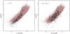 |
Fig. 13 Relation between 12+log(O/H) and log(N/O) for the star-forming selected SDSS galaxies (in brown) and for zCOSMOS for z < 0.2 (black dots in left hand panel) and for 0.2 < z < 0.42 (right hand panel). |
5. Summary and conclusions
We studied the cosmic evolution of the MZR from z ≈ 1.3 up to now using complete samples of star-forming galaxies: in the Local Universe we used the SDSS-DR7 and for higher z we used the 20 k zCOSMOS bright sample. The selection of star-forming objects and derivation of physical properties, including stellar masses, SFRs, oxygen abundances, and N/O, were performed using consistent methods. This is especially relevant in the case of the VIMOS spectra taken for the zCOSMOS sample since the set of available emission lines varies in each redshift regime. Two important aspects were considered when deriving chemical abundances: i) all strong-line methods used to derive 12+log(O/H) and log(N/O) were consistent with the Te-method as used in PMC09; and ii) the S/N threshold to select objects was put at a lower value to avoid possible selection effects in the final distributions of the derived properties.
The analysis of the evolution of the MZR in different redshift bins confirms an increase in the metallicity from z = 1.32, but the dispersion is too high to assess any variation in the shape of the MZR.
Considering the dependence of metallicity on SFR found by several authors, we derived an SFR-corrected MZR. This correction slighly reduces the dispersion of the MZR, but not noticeably since the dispersion in the SFR distributions is not very high. We still see the evolution of the metallicity for galaxies of the same stellar mass bin at different epochs, although this is slightly lower than for the MZR.
Finally, we studied the evolution of the MNOR taking the log(N/O) instead of (O/H) in the MZR. Since N/O was derived from the N2S2 parameter as calibrated by PMC09, we carried out this study for the zCOSMOS 20k sample only up to z ≈ 0.42. The main advantage to considering the MNOR with respect to the MZR is the independence of this relation on SFR, which confirms that the dependence of Z on SFR is probably due to inflows of metal-poor gas in some starburst events. In the studied redshift regime we still see the evolution of the chemical content of galaxies with the same stellar mass from younger ages of the Universe, confirming that the aforementioned evolution of the MZR is not just a selection effect of the observed objects at high z.
Available at http://www.mpa-garching.mpg.de/SDSS/
Acknowledgments
We thank C. Tremonti for having made the original platefit code available to the zCOSMOS collaboration. This work has been partially supported by the CNRS-INSU and its Programmes Nationaux de Galaxies et de Cosmologie (France), and by projects AYA2007-67965-C03-02 and AYA2010-21887-C04-01 of the Spanish National Plan for Astronomy and Astrophysics, and by the project TIC114 Galaxias y Cosmología of the Junta de Andalucía (Spain). The VLT-VIMOS observations were carried out on guarateed time (GTO) allocated by the European Southern Observatory (ESO) to the VIRMOS consortium, under a contractual agreement between the Centre National de la Recherche Scientifique of France, heading a consortium of French and Italian institutes, and ESO, to design, manufacture, and test the VIMOS instrument. The work was based on observations obtained with MegaPrime/MegaCam, a joint project of CFHT and CEA/DAPNIA, at the Canada-France-Hawaii Telescope (CFHT) which is operated by the National Research Council (NRC) of Canada, the Institut National des Science de l’Univers of the Centre National de la Recherche Scientifique (CNRS) of France and the University of Hawaii. This work is based in part on data products produced at TERAPIX and the Canadian Astronomy Data Centre as part of the Canada-France-Hawaii Telescope Legacy Survey, a collaboration project of NRC and CNRS. We finally thank José M. Vílchez and Ricardo Amorín for very fruitful discussions that have helped to reach some of the conclusions depicted in this work.
References
- Amorín, R. O., Pérez-Montero, E., & Vílchez, J. M. 2010, ApJ, 715, L128 [NASA ADS] [CrossRef] [Google Scholar]
- Bertoldi, F., Carilli, C., Aravena, M., et al. 2007, ApJS, 172, 132 [NASA ADS] [CrossRef] [Google Scholar]
- Bolzonella, M., Kovač, K., Pozzetti, L., et al. 2010, A&A, 524, A76 [NASA ADS] [CrossRef] [EDP Sciences] [Google Scholar]
- Bouché, N., Dekel, A., Genzel, R., et al. 2010, ApJ, 718, 1001 [NASA ADS] [CrossRef] [Google Scholar]
- Brinchmann, J., Charlot, S., White, S. D. M., et al. 2004, MNRAS, 351, 1151 [NASA ADS] [CrossRef] [Google Scholar]
- Brisbin, D., & Harwit, M. 2012, ApJ, 750, 142 [NASA ADS] [CrossRef] [Google Scholar]
- Brodie, J. P., & Huchra, J. P. 1991, ApJ, 379, 157 [NASA ADS] [CrossRef] [Google Scholar]
- Brooks, A. M., Governato, F., Booth, C. M., et al. 2007, ApJ, 655, L17 [NASA ADS] [CrossRef] [Google Scholar]
- Bruzual, G., & Charlot, S. 2003, MNRAS, 344, 1000 [NASA ADS] [CrossRef] [Google Scholar]
- Capak, P., Aussel, H., Ajiki, M., et al. 2007, ApJS, 172, 99 [NASA ADS] [CrossRef] [Google Scholar]
- Cardelli, J. A., Clayton, G. C., & Mathis, J. S. 1989, ApJ, 345, 245 [NASA ADS] [CrossRef] [Google Scholar]
- Charlot, S., & Longhetti, M. 2001, MNRAS, 323, 887 [NASA ADS] [CrossRef] [Google Scholar]
- Contini, T., Treyer, M. A., Sullivan, M., & Ellis, R. S. 2002, MNRAS, 330, 75 [NASA ADS] [CrossRef] [Google Scholar]
- Cowie, L. L., & Barger, A. J. 2008, ApJ, 686, 72 [NASA ADS] [CrossRef] [Google Scholar]
- Cresci, G., Mannucci, F., Sommariva, V., et al. 2012, MNRAS, 421, 262 [NASA ADS] [Google Scholar]
- Daddi, E., Dickinson, M., Morrison, G., et al. 2007, ApJ, 670, 156 [NASA ADS] [CrossRef] [Google Scholar]
- Davé, R., Finlator, K., & Oppenheimer, B. D. 2007, EAS Publ. Ser., 24, 183 [CrossRef] [EDP Sciences] [Google Scholar]
- Davé, R., Finlator, K., & Oppenheimer, B. D. 2012, MNRAS, 421, 98 [NASA ADS] [CrossRef] [Google Scholar]
- De Lucia, G., Kauffmann, G., & White, S. D. M. 2004, MNRAS, 349, 1101 [NASA ADS] [CrossRef] [Google Scholar]
- de Rossi, M. E., Tissera, P. B., & Scannapieco, C. 2007, MNRAS, 374, 323 [NASA ADS] [CrossRef] [Google Scholar]
- Denicoló, G., Terlevich, R., & Terlevich, E. 2002, MNRAS, 330, 69 [NASA ADS] [CrossRef] [Google Scholar]
- Edmunds, M. G. 1990, MNRAS, 246, 678 [NASA ADS] [Google Scholar]
- Edmunds, M. G., & Pagel, B. E. J. 1978, MNRAS, 185, 77 [NASA ADS] [CrossRef] [Google Scholar]
- Elbaz, D., Daddi, E., Le Borgne, D., et al. 2007, A&A, 468, 33 [NASA ADS] [CrossRef] [EDP Sciences] [Google Scholar]
- Erb, D. K., Shapley, A. E., Pettini, M., et al. 2006, ApJ, 644, 813 [NASA ADS] [CrossRef] [Google Scholar]
- Finlator, K., Davé, R., & Oppenheimer, B. D. 2007, MNRAS, 376, 1861 [NASA ADS] [CrossRef] [Google Scholar]
- Garnett, D. R., Shields, G. A., Skillman, E. D., Sagan, S. P., & Dufour, R. J. 1997, ApJ, 489, 63 [NASA ADS] [CrossRef] [Google Scholar]
- Hammer, F., Flores, H., Elbaz, D., et al. 2005, A&A, 430, 115 [NASA ADS] [CrossRef] [EDP Sciences] [Google Scholar]
- Hasinger, G., Cappelluti, N., Brunner, H., et al. 2007, ApJS, 172, 29 [NASA ADS] [CrossRef] [Google Scholar]
- Henry, R. B. C., Edmunds, M. G., & Köppen, J. 2000, ApJ, 541, 660 [NASA ADS] [CrossRef] [Google Scholar]
- Ilbert, O., Tresse, L., Arnouts, S., et al. 2004, MNRAS, 351, 541 [NASA ADS] [CrossRef] [Google Scholar]
- Kewley, L. J., & Ellison, S. L. 2008, ApJ, 681, 1186 [Google Scholar]
- Kewley, L. J., Dopita, M. A., Sutherland, R. S., Heisler, C. A., & Trevena, J. 2001, ApJ, [Google Scholar]
- Kewley, L. J., Groves, B., Kauffmann, G., & Heckman, T. 2006, MNRAS, 372, 961 [NASA ADS] [CrossRef] [Google Scholar]
- Kobulnicky, H. A., Kennicutt, R. C., Jr., & Pizagno, J. L. 1999, ApJ, 514, 544 [NASA ADS] [CrossRef] [Google Scholar]
- Kobulnicky, H. A., Willmer, C. N. A., Phillips, A. C., et al. 2003, ApJ, 599, 1006 [NASA ADS] [CrossRef] [Google Scholar]
- Koekemoer, A. M., Aussel, H., Calzetti, D., et al. 2007, ApJS, 172, 196 [NASA ADS] [CrossRef] [Google Scholar]
- Köppen, J., & Hensler, G. 2005, A&A, 434, 531 [NASA ADS] [CrossRef] [EDP Sciences] [Google Scholar]
- Köppen, J., Weidner, C., & Kroupa, P. 2007, MNRAS, 375, 673 [NASA ADS] [CrossRef] [Google Scholar]
- Lamareille, F. 2007, Ph.D. Thesis [Google Scholar]
- Lamareille, F., Mouhcine, M., Contini, T., Lewis, I., & Maddox, S. 2004, MNRAS, 350, 396 [NASA ADS] [CrossRef] [Google Scholar]
- Lamareille, F., Contini, T., Le Borgne, J.-F., et al. 2006, A&A, 417, 839 [Google Scholar]
- Lamareille, F., Brinchmann, J., Contini, T., et al. 2009, A&A, 495, 53 [NASA ADS] [CrossRef] [EDP Sciences] [Google Scholar]
- Lara-López, M. A., Cepa, J., Bongiovanni, A., et al. 2010, A&A, 521, L53 [NASA ADS] [CrossRef] [EDP Sciences] [Google Scholar]
- Le Fèvre, O., Saisse, M., Mancini, D., et al. 2003, Proc. SPIE, 4841, 1670 [NASA ADS] [CrossRef] [Google Scholar]
- Lee, H., Skillman, E. D., Cannon, J. M., et al. 2006, ApJ, 647, 970 [NASA ADS] [CrossRef] [Google Scholar]
- Lequeux, J., Peimbert, M., Rayo, J. F., Serrano, A., & Torres-Peimbert, S. 1979, A&A, 80, 155 [NASA ADS] [Google Scholar]
- Liang, Y. C., Hammer, F., Flores, H., et al. 2004, A&A, 423, 867 [NASA ADS] [CrossRef] [EDP Sciences] [Google Scholar]
- Liang, Y. C., Hammer, F., & Yin, S. Y. 2007, A&A, 474, 807 [NASA ADS] [CrossRef] [EDP Sciences] [Google Scholar]
- Lilly, S. J., Le Fèvre, O., Renzini, A., et al. 2007, ApJS, 172, 70 [NASA ADS] [CrossRef] [Google Scholar]
- Lilly, S. J., Le Brun, V., Maier, C., et al. 2009, ApJS, 184, 218 [Google Scholar]
- Liu, X., Shapley, A. E., Coil, A. L., Brinchmann, J. N., & Ma, C.-P. 2008, ApJ, 678, 758 [NASA ADS] [CrossRef] [Google Scholar]
- Maier, C., Meisenheimer, K., & Hippelein, H. 2004, A&A, 418, 475 [NASA ADS] [CrossRef] [EDP Sciences] [Google Scholar]
- Maier, C., Lilly, S. J., Carollo, C. M., Stockton, A., & Brodwin, M. 2005, ApJ, 634, 849 [NASA ADS] [CrossRef] [Google Scholar]
- Maier, C., Lilly, S. J., Carollo, C. M., et al. 2006, ApJ, 639, 858 [NASA ADS] [CrossRef] [Google Scholar]
- Maiolino, R., Nagao, T., Grazian, A., et al. 2008, A&A, 488, 463 [NASA ADS] [CrossRef] [EDP Sciences] [Google Scholar]
- Mannucci, F., Cresci, G., Maiolino, R., et al. 2009, MNRAS, 398, 1915 [NASA ADS] [CrossRef] [Google Scholar]
- Mannucci, F., Cresci, G., Maiolino, R., Marconi, A., & Gnerucci, A. 2010, MNRAS, 408, 2115 [NASA ADS] [CrossRef] [Google Scholar]
- Maraston, C. 2005, MNRAS, 362, 799 [NASA ADS] [CrossRef] [Google Scholar]
- Marocco, J., Hache, E., & Lamareille, F. 2011, A&A, 531, A71 [NASA ADS] [CrossRef] [EDP Sciences] [Google Scholar]
- McCracken, H. J., Capak, P., Salvato, M., et al. 2010, ApJ, 708, 202 [NASA ADS] [CrossRef] [Google Scholar]
- McGaugh, S. S. 1991, ApJ, 380, 140 [NASA ADS] [CrossRef] [Google Scholar]
- Moustakas, J., Zaritsky, D., Brown, M., et al. 2011, ApJ, submitted [arXiv:1112.3300] [Google Scholar]
- Nagao, T., Maiolino, R., & Marconi, A. 2006, A&A, 459, 85 [NASA ADS] [CrossRef] [EDP Sciences] [Google Scholar]
- Noeske, K. G., Weiner, B. J., Faber, S. M., et al. 2007, ApJ, 660, L43 [Google Scholar]
- Pagel, B. E. J., Edmunds, M. G., Blackwell, D. E., Chun, M. S., & Smith, G. 1979, MNRAS, 189, 95 [NASA ADS] [CrossRef] [Google Scholar]
- Perez, J., Michel-Dansac, L., & Tissera, P. B. 2011, MNRAS, 417, 580 [NASA ADS] [CrossRef] [Google Scholar]
- Pérez-Montero, E., & Contini, T. 2009, MNRAS (PMC09) [Google Scholar]
- Pérez-Montero, E., & Díaz, A. I. 2005, MNRAS, 361, 1063 [NASA ADS] [CrossRef] [Google Scholar]
- Pérez-Montero, E., Hägele, G. F., Contini, T., & Díaz, A. I. 2007, MNRAS, 381, 125 [NASA ADS] [CrossRef] [Google Scholar]
- Pérez-Montero, E., Contini, T., Lamareille, F., et al. 2009, A&A, 495, 73 [NASA ADS] [CrossRef] [EDP Sciences] [Google Scholar]
- Pettini, M., & Pagel, B. E. J. 2004, MNRAS, 348, L59 [NASA ADS] [CrossRef] [Google Scholar]
- Queyrel, J., Contini, T., Pérez-Montero, E., et al. 2009, A&A, 506, 681 [NASA ADS] [CrossRef] [EDP Sciences] [Google Scholar]
- Queyrel, J., Contini, T., Kissler-Patig, M., et al. 2012, A&A, 539, A93 [NASA ADS] [CrossRef] [EDP Sciences] [Google Scholar]
- Pilyugin, L. S., & Ferrini, F. 2000, A&A, 358, 72 [NASA ADS] [Google Scholar]
- Pilyugin, L. S., Thuan, T. X., & Vílchez, J. M. 2003, A&A, 397, 487 [NASA ADS] [CrossRef] [EDP Sciences] [Google Scholar]
- Pozzetti, L., Bolzonella, M., Lamareille, F., et al. 2007, A&A, 474, 443 [NASA ADS] [CrossRef] [EDP Sciences] [Google Scholar]
- Sakstein, J., Pipino, A., Devriendt, J. E. G., & Maiolino, R. 2011, MNRAS, 410, 2203 [NASA ADS] [CrossRef] [Google Scholar]
- Sanders, D. B., Salvato, M., Aussel, H., et al. 2007, ApJS, 172, 86 [Google Scholar]
- Savaglio, S., Glazebrook, K., Le Borgne, D., et al. 2005, ApJ, 635, 260 [NASA ADS] [CrossRef] [Google Scholar]
- Saviane, I., Ivanov, V. D., Held, E. V., et al. 2008, A&A, 487, 901 [NASA ADS] [CrossRef] [EDP Sciences] [Google Scholar]
- Schinnerer, E., Smolčić, V., Carilli, C. L., et al. 2007, ApJS, 172, 46 [NASA ADS] [CrossRef] [Google Scholar]
- Scoville, N., Aussel, H., Brusa, M., et al. 2007, ApJS, 172, 1 [NASA ADS] [CrossRef] [Google Scholar]
- Skillman, E. D., Kennicutt, R. C., & Hodge, P. W. 1989, ApJ, 347, 875 [NASA ADS] [CrossRef] [Google Scholar]
- Spergel, D. N., Verde, L., Peiris, H. V., et al. 2003, ApJS, 148, 175 [NASA ADS] [CrossRef] [Google Scholar]
- Storchi-Bergmann, T., Calzetti, D., & Kinney, A. L. 1994, ApJ, 429, 572 [NASA ADS] [CrossRef] [Google Scholar]
- Storey, P. J., & Hummer, D. G. 1995, MNRAS, 272, 41 [NASA ADS] [CrossRef] [Google Scholar]
- Taniguchi, Y., Scoville, N., Murayama, T., et al. 2007, ApJS, 172, 9 [NASA ADS] [CrossRef] [Google Scholar]
- Thuan, T. X., Pilyugin, L. S., & Zinchenko, I. A. 2010, ApJ, 712, 1029 [NASA ADS] [CrossRef] [Google Scholar]
- Torrey, P., Cox, T. J., Kewley, L., & Hernquist, L. 2012, ApJ, 746, 108 [NASA ADS] [CrossRef] [Google Scholar]
- Tremonti, C. A., Heckman, T. M., Kauffmann, G., et al. 2004, ApJ, 613, 898 [NASA ADS] [CrossRef] [Google Scholar]
- Yabe, K., Ohta, K., Iwamuro, F., et al. 2012, PASJ, 64, 60 [NASA ADS] [Google Scholar]
- Yates, R. M., Kauffmann, G., & Guo, Q. 2012, MNRAS, 422, 215 [NASA ADS] [CrossRef] [Google Scholar]
- Zahid, H. J., Kewley, L. J., & Bresolin, F. 2011, ApJ, 730, 137 [NASA ADS] [CrossRef] [Google Scholar]
- Zaritsky, D., Kennicutt, R. C., & Huchra, J. P. 1994, ApJ, 420, 87 [NASA ADS] [CrossRef] [Google Scholar]
All Tables
Relative number of star-forming galaxies and narrow-line AGNs in each redshift bin in the zCOSMOS bright sample.
Derived minimum masses (in log(M/M⊙)) for different redshift bins obtained for different levels of completeness.
Average offsets between the medians measured in the SDSS reference sample and for the star-forming galaxies of zCOSMOS 20k in each redshift bin for the mass − metallicity relation (MZR), the star formation-corrected mass − metallicity relation (SMZ), and the relation between stellas mass and N/O (MNOR).
All Figures
|
Fig. 1 Diagnostic diagrams used to select star-forming objects in the studied sample in each redshift range. From left to right and from up to down: [N ii]/Hα vs. [S ii]/Hα, [N ii]/Hα vs. [O iii]/Hβ, [O ii]/Hβ vs. [O iii]/Hβ, and [O ii]/Hβ vs. [Ne iii]Hβ. |
| In the text | |
|
Fig. 2 Relation between redshift and stellar mass (in solar masses) for the complete zCOSMOS 20 K sample (brown points) and star-forming selected galaxies (violet points). The solid lines show the logarithmic fitting to the limiting masses of the star-forming sample for levels 25%, 50%, and 75% of completeness. Lower and left hand panels also show the distributions for both the complete sample (empty histogram) and the star-forming galaxies (filled histogram) of z and M∗, respectively. |
| In the text | |
|
Fig. 3 Distribution of the calculated SFR for the star-forming galaxies of the SDSS (in black) and for zCOSMOS star-forming galaxies in different redshift bins (in red). The vertical lines show the medians for the whole zCOSMOS sample (in blue) and for each redshift range (in red). |
| In the text | |
|
Fig. 4 Distribution of the calculated 12+log(O/H) for the star-forming galaxies of the SDSS (black histogram) and zCOSMOS (red histograms) for different redshift bins. The vertical lines show the medians for the whole zCOSMOS sample (in blue) and for each redshift range (in red). |
| In the text | |
|
Fig. 5 Distribution of the calculated log(N/O) for the star-forming galaxies of the SDSS (black histogram) and zCOSMOS (red histograms) for different redshift bins. The vertical lines show the medians for the whole zCOSMOS sample (in blue) and for each redshift range (in red). |
| In the text | |
|
Fig. 6 Relation between stellar mass (in units of M⊙) and 12 + log (O/H) for the selected star-forming galaxies of the SDSS-DR7. The red solid line shows the quadratical fit to the medians in bins of 0.2 dex of stellar mass. |
| In the text | |
|
Fig. 7 Cosmic evolution of the MZR for six different redshift bins increasing from left to right and from up to down. The red solid line shows the fit to the MZR in the SDSS data. Grey areas show the ± σ intervals to the Z medians fits in different mass bins for each redshift range. The vertical lines show the minimum masses for 25%, 50% and 75% levels of completeness. Red crosses represent low-Z objects in the sample found using ISAAC near-IR observations (Maier et al., in prep.). |
| In the text | |
|
Fig. 8 To the left MZR and quadratical fits for different bins of log SFR. To the right, same plot for the relation between log (N/O) and stellar mass. |
| In the text | |
|
Fig. 9 Relation between stellar mass in units of M⊙ and 12+log(O/H) with the correction depending on log(SFR) for the star-forming selected galaxies of the SDSS-DR7. The red solid line shows the quadratical fit to the medians in bins of 0.2 dex of stellar mass. |
| In the text | |
|
Fig. 10 Cosmic evolution of the SFR-corrected MZR for six different redshift bins increasing from left to right and from up to down. The red solid line shows the fitting to the SMZ in the SDSS data. Upper and lower solid lines show the ± σ intervals to the fitting to the y medians in different mass bins for each redshift range. The vertical lines show the minimum mass limits for 25%, 50% and 75% levels of completeness. Red crosses represent low-Z objects in the sample found using ISAAC near-IR observations (Maier et al., in prep.). |
| In the text | |
|
Fig. 11 Relation between stellar mass in units of M⊙ and log(N/O) for the star-forming selected galaxies of the SDSS-DR7. The red solid line shows the quadratical fit to the medians in bins of 0.2 dex of stellar mass. |
| In the text | |
|
Fig. 12 Cosmic evolution of the MNOR for two different redshift bins. The red solid line shows the fit to the MNOR in the SDSS data. Upper and lower solid lines show the ± σ intervals to the fitting to the N/O medians in different mass bins for each redshift range. The vertical lines show the minimum mass limits for 25%, 50% and 75% levels of completeness. |
| In the text | |
|
Fig. 13 Relation between 12+log(O/H) and log(N/O) for the star-forming selected SDSS galaxies (in brown) and for zCOSMOS for z < 0.2 (black dots in left hand panel) and for 0.2 < z < 0.42 (right hand panel). |
| In the text | |
Current usage metrics show cumulative count of Article Views (full-text article views including HTML views, PDF and ePub downloads, according to the available data) and Abstracts Views on Vision4Press platform.
Data correspond to usage on the plateform after 2015. The current usage metrics is available 48-96 hours after online publication and is updated daily on week days.
Initial download of the metrics may take a while.