© ESO, 2012

1. Introduction

The internal structure of red giants bears the history of their evolution. They are therefore seen as key for the understanding of stellar evolution. They are expected to have a rapidly rotating core and a slowly rotating envelope (e.g. Sills & Pinsonneault 2000), as a result of internal angular momentum distribution. Indirect indications of the internal angular momentum are given by surface-abundance anomalies resulting from the action of internal transport processes and from the redistribution of angular momentum and chemical elements (Zahn 1992; Talon & Charbonnel 2008; Maeder 2009; Canto Martins et al. 2011). Direct measurements of the surface rotation are given by the measure of v sini (e.g. Carney et al. 2008). The slow rotation rate in low-mass white dwarfs (e.g. Kawaler et al. 1999) suggests a spinning down of the rotation during the red giant branch (RGB) phase. In addition, 3D simulations show non-rigid rotation in the convective envelope of red giants (Brun & Palacios 2009). Different mechanisms for spinning down the core have been investigated (e.g. Charbonnel & Talon 2005). Rotationally-induced mixing, amid other angular momentum transport mechanisms, is still poorly understood but is known to take place in stellar interiors. Therefore, a direct measurement of rotation inside red giants would give us an unprecedented opportunity to perform a leap forward on our understanding of angular momentum transport in stellar interiors (e.g. Lagarde et al. 2012; Eggenberger et al. 2012).

This is becoming possible with seismology, which provides us with direct access to measure the internal rotation profile, as shown by Beck et al. (2012) and Deheuvels et al. (2012a). They demonstrate that it is possible to measure the core rotation thanks to the precision of asteroseismic results derived from the photometric light curves of red giants provided by the NASA Kepler mission (Borucki et al. 2010). Previous work on field star asteroseismic surveys shows that is possible to define evolutionary sequences (e.g. Miglio et al. 2009; Huber et al. 2011). So, with ensemble asteroseismology, we aim to get measurements in a large enough sample of red giants to explore the variation of the internal rotation with evolution.

After a decade of relatively uncertain ground-based measurements, CoRoT has unambiguously revealed that red giants show solar-like oscillations (De Ridder et al. 2009). Important scaling relations have then been shown (Hekker et al. 2009) for deriving crucial information on the stellar mass and radius from global seismic parameters (Kallinger et al. 2010). Specific features of solar-like oscillations in red giants have been characterized (e.g. Bedding et al. 2010; Mosser et al. 2010; Huber et al. 2010). Mixed modes, which correspond to the coupling of gravity waves in the radiative core region and pressure waves in the envelope (Dziembowski et al. 2001; Dupret et al. 2009), have been detected in red giants. They were first reported by Bedding et al. (2010). Their period spacings were measured by Beck et al. (2011). Bedding et al. (2011) and Mosser et al. (2011a) have shown the capability of these modes to measure the evolutionary status of red giants. Mixed modes can be divided into two categories, namely gravity-dominated mixed modes (hereafter called g-m modes) which have large amplitudes in the core, and, in contrast, pressure-dominated mixed modes (p-m modes). The frequencies of the p-m modes are very close to the theoretical pure p mode frequencies; they however appear to have a significant g component, and are therefore sensitive also to the core conditions. We analyse in this work mostly stars showing a rich mixed-mode spectrum.

Observations and data are presented in Sect. 2. The observed properties of the rotational splittings are described in Sect. 3. In Sect. 4, we derive scaling relations governing the rotational splitting, independent of any modeling, but based on the observational evidence of a much higher rotation rate in the stellar core. The way the core rotation is related to the measured rotational splitting is quantified in Sect. 5. In Sect. 6, we then derive unique information on the core rotation in red giants and probe their internal angular momentum and its evolution.

2. Data

2.1. 25-month long observation

The red giant stars analyzed in this work have already been presented (e.g. Hekker et al. 2011, and references therein). We now benefit from longer time series. All red giants observed up to Kepler’s quarter Q10 have been analyzed. Original light curves were processed according to Jenkins et al. (2010) and corrected according to the procedure of García et al. (2011). The Fourier analysis of the 868-day long time series provides a frequency resolution of about 11.5 nHz. Due to the characteristics of the measurement, we have in principle access to rotation periods up to the observation duration. For a few RGB stars showing large rotational splittings, a reprocessed set of Q0 to Q11 Kepler data has been used, based on the extraction of the stellar fluxes using new custom masks from the recently released pixel-data information (Bloemen et al. 2012). These new light curves were then corrected applying the algorithms developed by García et al. (2011) but using a refined new automatic procedure (Mathur et al., in prep.). In practice, we measure rotational splittings with periods in the range 8–280 days.

2.2. Mixed-mode pattern

The complete identification of the red giant pressure oscillation pattern is given by the description of the so-called universal oscillation pattern (Mosser et al. 2011b). This method alleviates any problem of mode identification. The whole frequency pattern of pure p modes is approximated by: ${\mathit{\nu }}_{{\mathit{n}}_{\mathrm{p}}\mathit{,\ell }}\mathrm{=}\left({\mathit{n}}_{\mathrm{p}}\mathrm{+}\frac{\mathit{\ell }}{\mathrm{2}}\mathrm{+}\mathit{\epsilon }\mathrm{-}{\mathit{d}}_{\mathrm{0}\mathit{\ell }}\mathrm{+}\frac{\mathit{\alpha }}{\mathrm{2}}\mathrm{[}{\mathit{n}}_{\mathrm{p}}\mathrm{-}{\mathit{n}}_{\max }{\mathrm{]}}^{\mathrm{2}}\right)\mathrm{\Delta }\mathit{\nu ,}$(1)where Δν is the mean large separation measured in a broad frequency range around the frequency ν_max of maximum power, n_p is the p-mode radial order, ℓ is the angular degree, ε is the phase offset, d_0ℓ accounts for the so-called small separation, α is a small constant, and n_max = ν_max/Δν. The parameters ε, d_0ℓ and α are considered as a function of the large separation; an updated fit of ε is used, comparable to the expression of Corsaro et al. (2012). The parameter α represents the second-order term of the asymptotic development (Tassoul 1980) and accounts for the mean curvature of the radial mode oscillation pattern (Mosser et al. 2012a). It was considered as a constant by Mosser et al. (2011b). Here, with much longer time series and large separations observed up to 20 μHz, we prefer to use the fit $\mathit{\alpha }\mathrm{=}\mathrm{0.015}\mathrm{\Delta }{\mathit{\nu }}^{-0.32}\mathit{,}$(2)with Δν in μHz. This relation is derived from the detailed analysis of the radial modes with the method presented by Mosser (2010).

The recent analysis of Kallinger et al. (2012) has shown that this development is valid, independent of the stellar evolutionary status, under the condition that the determination of the large separation is global and not local. Their Fig. 6 illustrates the important curvature of the ridges depicted by the quadratic term of Eq. (1). The comparative work by Hekker et al. (2012) shows that the extra hypothesis used by Mosser et al. (2011b), expressed by the function ε(Δν), helps to obtain very precise results. Using this constraint requires fitting each oscillation spectrum in a large frequency range around ν_max and taking into account the mean curvature of the p-mode oscillation pattern.

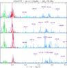Fig. 1 Échelle diagram of a typical RGB star (KIC 6144777) as a function of ν/Δν − (np + ε). The radial order np is indicated on the y-axis. Radial modes (highlighted in red) are centered on 0, quadrupole modes (highlighted in green), near − 0.12 (with a radial order np − 1), and ℓ = 3 modes, sometimes observed, (highlighted in light blue) near 0.20. Dipole mixed modes are identified with the frequency given by the asymptotic relation of mixed modes, in μHz. The fit is based on peaks showing a height larger than eight times the mean background value (grey dashed lines).

Equation (1) holds precisely for radial modes and gives a proxy for the pure pressure dipole (ℓ = 1) modes. However, due to the significant coupling of pressure waves with gravity waves in the inner radiative region, the dipole oscillation pattern is dominated by mixed modes located around the position of the pure p mode. The frequency interval between the individual mixed modes is not constant and is determined according to the method presented in Mosser et al. (2011a). For stars showing a large number of g-m modes, the oscillation pattern can be precisely described by an asymptotic relation presented by Goupil et al. (2012), following the ideas originally developed by Shibahashi (1979) and Unno et al. (1989). We apply this method, as explained in Mosser et al. (2012c), in order to locate precisely the dipole mixed modes.

The échelle diagram of Fig. 1 shows the identification of the radial modes provided by Eq. (1), with the mode curvature, and the location of the mixed ℓ = 1,m = 0 modes defined by the asymptotic relation. The remaining shifts between the actual and expected peaks positions, due for instance to a sharp structure variation (Miglio et al. 2010), are small compared to the mixed mode spacings. Hence, they do not hamper the mode identification.

3. Measuring the rotational splittings

From the analysis of dipole mixed modes, Beck et al. (2012) showed differential rotation in red giants. In this section, we propose a model for describing the rotational splittings of dipole mixed modes and an automated method for measuring them.

3.1. Modulation of rotational splittings

Because of differential rotation, a simple interpretation of rotational splittings in terms of mean rotation of the star is inadequate. The situation is made even more complicated by the fact that rotational splittings are measured for dipole mixed modes. Indeed, the mixed nature of the modes varies as a function of mode frequency, as shown by Dupret et al. (2009). As a result of those two interlaced effects, Mosser et al. (2012c) have shown that rotational splittings are modulated in frequency, with a period of Δν. The rotational splitting can be written $\mathit{\delta }{\mathit{\nu }}_{\mathrm{split}}\mathrm{=}{\mathit{\nu }}_{\mathit{n,}\mathrm{1}\mathit{,m}}\mathrm{-}{\mathit{\nu }}_{\mathit{n,}\mathrm{1}}\mathrm{=}\mathit{m}\mathrm{ℛ}\mathrm{\left(}\mathit{\nu }\mathrm{\right)}\mathit{\delta }{\mathit{\nu }}_{\mathrm{rot}}\mathit{,}$(3)where m is the azimuthal order and δν_rot is the maximum value observed for g-m modes. Locally, around the position of a pure dipole p mode of radial order n_p, Mosser et al. (2012c) have shown that ℛ can be empirically expressed as: 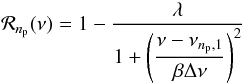${\mathrm{ℛ}}_{{\mathit{n}}_{\mathrm{p}}}\mathrm{\left(}\mathit{\nu }\mathrm{\right)}\mathrm{=}\mathrm{1}\mathrm{-}\frac{\mathit{\lambda }}{\mathrm{1}\mathrm{+}{\left(\frac{\mathit{\nu }\mathrm{-}{\mathit{\nu }}_{{\mathit{n}}_{\mathrm{p}}\mathit{,}\mathrm{1}}}{\mathit{\beta }\mathrm{\Delta }\mathit{\nu }}\right)}^{\mathrm{2}}}$(4)for a mixed mode with frequency ν associated with the pressure radial order n_p. The development, solely derived from the observed splittings, has currently no theoretical basis: the Lorentzian form has been chosen similar to the observed variation of the mixed-mode spacing with frequency (Beck et al. 2011; Bedding et al. 2011).

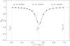Fig. 2 Empirical rotation profile ℛnp for dipole mixed modes associated to the pure p mode of radial order np, as a function of the reduced frequency ν/Δν − (np + ε).

The form of ℛ (Fig. 2) implies that the splittings are not symmetric, consistent with the findings of Deheuvels et al. (2012b). For multiplets near p-m modes, the closest component to the theoretical pure p mode has the smallest splitting. The asymmetry is expressed when considering Eq. (3) as an implicit equation, the splitting of the frequency ν_n,1,m compared to the non-rotating reference ν_n,1 depending on ν_n,1,m: ${\mathit{\nu }}_{\mathit{n,}\mathrm{1}\mathit{,m}}\mathrm{=}{\mathit{\nu }}_{\mathit{n,}\mathrm{1}}\mathrm{+}\mathit{m}\mathrm{ℛ}\mathrm{\left(}{\mathit{\nu }}_{\mathit{n,}\mathrm{1}\mathit{,m}}\mathrm{\right)}\mathit{\delta }{\mathit{\nu }}_{\mathrm{rot}}\mathit{.}$(5)It assumes, as observed but with the limitation of the observed frequency resolution, that the modulation of the splitting is the same for all radial orders. In fact, the fits of the splittings, obtained by supposing that the frequency of the m = 0 component of the dipole mixed modes is given by the asymptotic development, show that the terms λ and β are independent of the frequency. Furthermore, we have verified that the values of λ and β are always very close to 0.5 and 0.08, respectively, and hence do not depend on the evolutionary stage.

Due to the large volume of data, we need an automated method for deriving the rotational splittings, similar to the determination of the global seismic parameters Δν and ν_max (e.g. Hekker et al. 2011; Verner et al. 2011). This method has to cope with an interweaving of rotational splittings and mixed-mode spacings.

3.2. EACF analysis

We can use the envelope autocorrelation function (EACF) method (Mosser & Appourchaux 2009) to measure the rotational splittings of non-radial modes. This method was developed to measure the frequency spacing corresponding to the large separation of solar-like oscillations. With narrow filters centered on the expected ℓ = 1 pressure modes, it gives the spacing due to the mixed-mode pattern (Mosser et al. 2011a). With ultra-narrow filters centered on each individual mixed mode, it proves to be able to measure the rotational splittings. The central positions of the filters are chosen within the frequency ranges where mixed modes are expected. Each range is wider than half the large separation Δν, as shown by Mosser et al. (2012b). Different central positions of the filters are tested within this range, independent of the mixed-mode positions. The widths of the filters have to be narrow enough to select only one mixed mode, in order to avoid confusion between the g-mode spacing and the rotational splitting (Fig. 3). They are varied, in order to test a large range of splittings. We have tested five different widths, of the order of 1 μHz or less, which encompass the observed values.

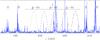Fig. 3 Zoom on the oscillation spectrum of the target KIC 10777816. Different narrow filters centered in the ℓ = 1 mixed mode range, indicated with different line styles, allow us to measure a local rotational splitting in each filter. For clarity, only those filters centered on possible multiplets have been represented.

In the EACF method, the signature of any comb-like structure in the spectrum, here the rotational splitting, is provided by the highest peak in the spectrum of the windowed spectrum. The signal is normalized in such a way that the mean white-noise level is 1. The reliability of the detection is derived from an H0 test. Since we use ultra-narrow filters, only high signal-to-noise time series can be analyzed.

For each filter width, multiplets were searched in seven radial orders around ν_max, at ten different positions per radial order. As a consequence, seventy possible signatures of the rotational splittings are analysed for a given filter. The criterion for a positive detection is the measurement of similar splittings for at least three positions centered on different dipole mixed modes corresponding to different radial orders n_p, with a signature of the EACF above the threshold level (Mosser & Appourchaux 2009). In order to account for the modulation of ℛ towards p-m modes (Fig. 2), we allow relative differences of 1/3 between the individual measurements. This threshold level has been determined empirically. It takes into account the fact that splittings are measured mainly in the wings of the function ℛ: the splittings of p-m modes are not easily measured, due to their shorter lifetime, whereas the amplitudes of the g-m modes located far from the p-m modes are too low to give a reliable signature.

3.3. Performance

All results found by the automated method have been verified individually by visually comparing the spectrum with itself after a shift corresponding to the rotational splitting. The method appeared to be dominated by g-m modes since they have narrower widths and are more numerous than p-m modes. Hence, they contribute much more efficiently to the EACF signature, as shown by the careful examination of numerous individual spectra. Therefore, the method mainly gives the rotational signature of the core. This is also clear from the close examination of the extracted splittings.

For stars with a low signal-to-noise ratio oscillation spectrum, generally faint stars or stars with low ν_max, we sometimes obtain spurious results. These results are clearly caused by the stochastic nature of the oscillation excitation, which occasionally resembles the complex pattern of multiple peaks shown by the dipole mode, and were discarded. Finally, depending on the stellar inclination i, the multiplets have two components (when sini is close to 1), three components (intermediate i values), or only one component (low i). In this latter case, measuring the splitting is not possible. The correct identification of the multiplets has been possible in most of the cases, allowing us to remove the confusion between δν_split and 2δν_split.

Possible confusion between rotational splittings and mixed-mode spacings has been investigated. Such a confusion is usually eliminated by limiting the width of the filter. However, RGB stars may show a rotational splitting very close to the g-mode spacing. We therefore explored the frequency domain where the solutions are ambiguous. Ambiguous detections are identified by the fact that, even if the rotational splitting and the mixed-mode spacing are both modulated in frequency, with a period Δν, their signatures are different. On the one hand, the g-mode frequency spacing varies as ν² since it approximately corresponds to a regular spacing in period (Bedding et al. 2011; Mosser et al. 2012c); on the other hand, the modulation ℛ is the same all along the spectrum (Eq. (4)).

As expected, the automated method fails when the rotational splittings are larger than half the mixed-mode spacings. This occurs for giants ascending the RGB, with Δν ≤ 12μHz. For these stars, a dedicated method, presented in the next paragraph, is needed to disentangle the rotational splittings from the mixed-mode spacings. We finally measured reliable rotational splittings in 265 red giants with the automated method, in the clump and in the early stages of the RGB. The combined effect of the tiny width of the filter and of the limited frequency resolution makes the method much more precise at high frequency than at low frequency. The relative precision is of about 5% in δν_rot for stars with Δν = 15 μHz and 25% when Δν = 5 μHz.

3.4. Validation with direct measurements

The values of the rotational splitting provided by the EACF method can be compared to a direct fit of the modulation of the splitting based on Eqs. (4) and (3). A tutorial for fitting the rotational multiplets is given in Appendix A; different fits are shown, in order to illustrate cases with rotational splittings lower, comparable or larger than the mixed-mode spacings. Using such fits, we measured the rotational splitting δν_rot in 102 red giants. Among them, 54 had already a rotational splitting measured with the EACF method. The remaining 48 stars had rotational splittings too large compared to the mixed modes spacings to be measurable with the EACF method. As a result, the total number of red giant stars with splittings measured with one or the other method is 313 (=265 + 102 − 54). The analysis of the detection and non-detection as a function of the large separation is summarized in Table 1. Non-detection at large Δν occurs for RGB stars with depressed mixed modes (identified by Mosser et al. 2012b) or with very low inclination. In this latter case, the components m = ± 1 are too low to allow the identification of multiplets. At small Δν, the non-detection is explained by the limited frequency resolution, but also by the poorer quality of the spectra, as expressed by the EACF coefficient (Mosser & Appourchaux 2009). For Δν in the ranges [4, 5 μHz] and [5, 6 μHz], the success of the detection depends mainly on the evolutionary status: small rotational splittings in clump stars with large mixed-mode spacings can be detected more easily than larger rotational splittings of RGB stars embedded in narrow spacings. We expect the number of positive detections to increase with prolonged observations: the frequency resolution will give access to rotational splittings in the upper RGB, and the better signal-to-noise ratio will allow the identification of tiny m = ± 1 components at low stellar inclination.

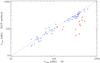Fig. 4 Comparison of the splittings measured with the EACF automated method to the splittings measured with the fit of the mixed modes (Eq. (4)). Red asterisks correspond to rotational splittings too large to be accurately measured in an automated way and hence excluded from the sample.

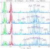Fig. 5 Zoom on the rotational splittings of the mixed modes corresponding to the radial orders np = 8 → 11 in the giant KIC 9574650, in an échelle diagram as a function of the reduced frequency ν/Δν − (np + ε). All triplets (m = −1,0,1) are identified with the function ℛ defined by Eq. (4). At low frequency, multiplets are overlapping.

We have noted that the automated EACF approach provides values that are 10% smaller than δν_rot derived from the individual fits (Fig. 4). This small correction is consistent with the different principles of the methods: the inferred value of δν_rot from Eqs. (3) and (4) is larger than any observed splitting, whereas the EACF method, even if dominated by g-m modes, also includes narrower multiplets in the vicinity of the p-m modes. This indicates that the 10% difference can be considered as a bias of the automated method. For homogeneity, all splittings obtained with the EACF method have been multiplied by a factor 1.10.

We have tested that the differential-rotation term ℛ of Eq. (4) holds for red giants in all stages of their evolution. Residuals of the fit of the splittings are much smaller than δν_rot. We observe a coefficient λ (Eq. (4)) of 0.5 ± 0.1 for an early RGB star such as KIC 7341231 studied by Deheuvels et al. (2012a), with Δν = 28.9μHz, as well as for clump stars with Δν ≃ 4.0μHz. The parameter β is about 0.08 ± 0.015 for all giants, except a very small number of exceptions, at the bottom of the RGB. Measuring a modulation profile ℛ almost independent of the evolution may indicate that its origin obeys to generic properties, similar for all red giants ascending the red giant branch (RGB).

For clump stars and early RGB stars, we note that the rotational splittings are significantly smaller than the mixed-mode spacings. In these cases, the individual fits confirm the automated measurement. However, when the rotational splittings are larger than the mixed-mode spacings, the EACF method was ineffective for extracting the correct large splitting: it derived wrong values that result from a combination of the mixed-mode spacing and rotational splitting. Application of Eq. (4) allowed us to provide the correct splittings even with large values comparable to the mixed-mode spacing. We stress that, in practice, it seems impossible to disentangle such multiplets from the mixed-mode pattern without the use of the asymptotic relation of mixed modes. We were able to investigate complicated cases, with rotational splittings significantly larger than the mixed-mode spacings, for RGB stars with Δν down to 7 μHz. Finally, even in the case where multiplets overlap, that is ν_{nm + 1,1, −1} < ν_nm,1, +1, with n_m the mixed-mode order, we do not observe any modification of the profile ℛ (Fig. 5). This indicates the absence of avoided crossings between dipole mixed modes with consecutive mixed-mode orders n_m and different azimuthal orders m. In other words, this shows the absence of coupling between such modes.

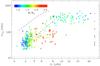Fig. 6 Rotational splitting δνrot as a function of the large separation Δν, in log-log scale. The dotted line indicates the frequency resolution. The dashed and dot-dashed lines represent the confusion limit with mixed modes in RGB and clump stars, respectively, derived from Mosser et al. (2012c). Crosses correspond to RGB stars, triangles to clump stars, and squares to secondary clump stars. The color code gives the mass estimated from the asteroseismic global parameters. The vertical bars indicate the mean error bars, as a function of the rotational splitting.

4. Scaling relations

We have derived estimates of the stellar mass and radius from the seismic global parameters and from the effective temperatures given by the Kepler Input Catalog (Brown et al. 2011), so that we can present the rotational splitting as a function of the stellar radius R (Fig. 7). The evolutionary status of the stars was determined by Mosser et al. (2012c). Among the helium-burning stars, we consider those with a mass greater than 1.8 M_⊙ to belong to the secondary clump. The uncertainties arising from the effective temperatures and the imprecision of the scaling relations do not impact the following analysis.

4.1. Rotational splittings δν_rot

Rotational splittings δν_rot are shown as a function of the large separation Δν (Fig. 6). We see that the detection is difficult at low Δν, due to the limited frequency resolution. This precludes an analysis of the core rotation in the high-luminosity RGB stars, but allows us to measure rotation in the clump stars.

We first consider the RGB stars, indicated by crosses in Fig. 6. We note that the rotational splitting slightly decreases when Δν decreases, that is, when the star evolves on the RGB. For clump stars and secondary clump stars, splittings are much smaller. At this stage, ensemble asteroseismology indicates either that the core rotation spins down, or that the splitting of g-m modes is not dominated by the core rotation. This last result is unlikely since g-m mode splittings are significantly larger than p-m mode splittings (Fig. 3), consistent with the observations reported by Beck et al. (2012) and Deheuvels et al. (2012a) for four early RGB stars.

4.2. Scaling relations

We have examined how the rotational splittings evolve with the stellar radius along the RGB (Fig. 7). Only RGB stars with a mass in the range [1.2, 1.5 M_⊙] were considered, to avoid a bias from the fact that high-mass stars are under-represented in the early stages of the RGB, whereas low-mass giants are under-represented in the later stages. With 49 RGB stars in this case, we find $\mathit{\delta }{\mathit{\nu }}_{\mathrm{rot}}\mathrm{\propto }{\mathit{R}}^{\mathrm{-}\mathrm{0.5}\hspace{0.17em}\mathrm{\pm }\hspace{0.17em}\mathrm{0.3}}\mathrm{\left(}\mathrm{RGB}\mathrm{\right)}\mathrm{.}$(6)In the first stages of the RGB, the splittings δν_rot show a slow decrease. Assuming the local conservation of angular momentum, such a decrease seems in contradiction with the core contraction: this has to be investigated.

The same exercise can be done for the clump stars. The fit, conducted over a much broader range of mass (Mosser et al. 2012c), gives $\mathit{\delta }{\mathit{\nu }}_{\mathrm{rot}}\mathrm{\propto }{\mathit{R}}^{\mathrm{-}\mathrm{1.3}\hspace{0.17em}\mathrm{\pm }\hspace{0.17em}\mathrm{0.4}}\mathrm{\left(}\mathrm{clump}\mathrm{\right)}\mathrm{or}\mathrm{\propto }{\mathit{R}}^{\mathrm{-}\mathrm{1.4}\hspace{0.17em}\mathrm{\pm }\hspace{0.17em}\mathrm{0.4}}\mathrm{\left(}\mathrm{2}\mathrm{ndclump}\mathrm{\right)}\mathrm{.}$(7)This indicates a different behaviour compared to RGB stars. We first note that the slopes are independent of the stellar mass. Closer to  − 2 than for RGB stars, they certainly relate the influence of the stellar expansion. We also note that secondary clump stars, which are more massive, show larger splittings than clump stars.

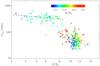Fig. 7 Rotation splitting δνrot as a function of the asteroseismic stellar radius, in log-log scale. Same symbols and color code as in Fig. 6. The dotted line indicates a splitting varying as R-2. The dashed (dot-dashed, triple-dot-dashed) line corresponds to the fit of RGB (clump, secondary clump) splittings.

4.3. Intermediate conclusions

From the analysis of the rotational splittings with the stellar radius, we note the weak decrease of RGB stars. According to the exponent of the fit reported by Eq. (6), this g-m mode splitting cannot be related to the surface rotation if it evolves at constant local angular momentum. The large change in the rotation evolution from the RGB to the clump can be related to the expansion of the non-degenerate helium burning core (Iben 1971; Sills & Pinsonneault 2000). This increase of the core radius is however limited and cannot explain the entire observed decrease of the rotational splittings, so that we are left with the most plausible conclusion that the strong decrease of the rotational splitting is the signature of a significant transfer of internal angular momentum from the inner to the outer layers. This transfer should preferably occur at the tip of the RGB, out of reach with current Kepler observations due to a limited frequency resolution. One could also imagine that the rotational splittings are sensitive to different layers, depending on the evolutionary status. This is investigated in the next section, where we aim to interpret the signification of the observed splittings δν_rot.

5. Linking the rotational splittings to the core rotation

To go a step further, we intend to qualitatively link the observed rotational splittings to the rotation inside the red giants.

5.1. Linear rotational splittings and average rotation

We assume that the rotation is slow enough that a first-order perturbation theory is sufficient to compute the rotational splittings. This yields the following expression for rotational splittings (Ledoux 1951; Christensen-Dalsgaard & Frandsen 1983; Christensen-Dalsgaard & Berthomieu 1991; Goupil 2009; Goupil et al. 2012) $\mathit{\delta }{\mathit{\nu }}_{\mathrm{rot}}{\mathit{,n,\ell }}_{}\mathrm{=}{\mathrm{\int }}_{\mathrm{0}}^{\mathrm{1}}{\mathrm{𝒦}}_{\mathit{n,\ell }}\mathrm{\left(}\mathit{x}\mathrm{\right)} \frac{\mathrm{\Omega }\mathrm{\left(}\mathit{x}\mathrm{\right)}}{\mathrm{2}\mathit{\pi }}\mathrm{d}\mathit{x,}$(8)where x = r/R is the normalized radius and Ω is the angular rotation (in rad/s). The rotational kernel of the mode of radial order n and angular degree ℓ takes the form ${\mathrm{𝒦}}_{\mathit{n,\ell }}\mathrm{=}\frac{\mathrm{1}}{{\mathit{I}}_{\mathit{n,\ell }}}[{\mathit{\xi }}_{\mathrm{r}}^{\mathrm{2}}\mathrm{+}\mathrm{(}\mathrm{\Lambda }\mathrm{-}\mathrm{1}\mathrm{)}{\mathit{\xi }}_{\mathrm{h}}^{\mathrm{2}}\mathrm{-}\mathrm{2}{\mathit{\xi }}_{\mathrm{r}}{\mathit{\xi }}_{\mathrm{h}}{]}_{\mathit{n,\ell }} \mathit{\rho }{\mathit{x}}^{\mathrm{2}}$(9)where I_n,ℓ is the mode inertia ${\mathit{I}}_{\mathit{nl}}\mathrm{=}{\mathrm{\int }}_{\mathrm{0}}^{\mathrm{1}} [{\mathit{\xi }}_{\mathit{r}}^{\mathrm{2}}\mathrm{+}\mathrm{\Lambda }{\mathit{\xi }}_{\mathit{h}}^{\mathrm{2}}{]}_{\mathit{n,\ell }} \mathit{\rho }{\mathit{x}}^{\mathrm{2}}\mathrm{d}\mathit{x}\mathit{.}$(10)The quantities entering these equations are the fluid vertical and horizontal displacement eigenfunctions, ξ_r, ξ_h respectively; ρ is the density, and Λ = ℓ(ℓ + 1).

The mode inertia is much larger for g-m modes that have a large amplitude in the inner cavity than for p-m modes. For a red giant, several mixed modes exist in the frequency vicinity of each radial mode. As a result, the variation with frequency of the dipole mode inertia shows a regular variation with a periodicity roughly equal to the large separation (see Dziembowski et al. 2001; Dupret et al. 2009; Christensen-Dalsgaard 2011; Goupil et al. 2012). This has been observationally confirmed (Mosser et al. 2012c). The linear rotational splittings (Eq. (8)) are found to follow closely the same behavior as the mode inertia for the same reason. However a significant amplification of the variation of the splittings with frequency compared to that of mode inertia should exist when the rotation is large in the central region (Goupil et al. 2012).

Because the red giants are characterized by an inner dense region and an outer envelope, it is convenient to consider the rotational splittings as the sum of two contributions $\mathit{\delta }{\mathit{\nu }}_{\mathrm{rot}}{\mathit{,n,\ell }}_{}\mathrm{=}\frac{\mathrm{1}}{\mathrm{2}\mathit{\pi }}(\mathrm{⟨}{\mathrm{\Omega }}_{\mathrm{K}}{\mathrm{⟩}}_{\mathrm{core}\mathit{,}\hspace{0.17em}\mathit{n,\ell }}\mathrm{+}\mathrm{⟨}{\mathrm{\Omega }}_{\mathrm{K}}{\mathrm{⟩}}_{\mathrm{env}\mathit{,}\hspace{0.17em}\mathit{n,\ell }})\mathit{,}$(11)where  ⟨ Ω_K ⟩ _{core, n,ℓ} is the angular rotation, weighted by the kernel, averaged over the central layers enclosed within a radius r_core and  ⟨ Ω_K ⟩ _env, n,ℓ the angular rotation averaged over the layers above x_core = r_core/R, 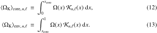$\begin{array}{ccc}\mathrm{⟨}{\mathrm{\Omega }}_{\mathrm{K}}{\mathrm{⟩}}_{\mathrm{core}\mathit{,}\hspace{0.17em}\mathit{n,\ell }}& \mathrm{\equiv }& \\ \mathrm{⟨}{\mathrm{\Omega }}_{\mathrm{K}}{\mathrm{⟩}}_{\mathrm{env}\mathit{,}\hspace{0.17em}\mathit{n,\ell }}& \mathrm{\equiv }& {\mathrm{\int }}_{{\mathit{x}}_{\mathrm{core}}}^{\mathrm{1}}\mathrm{\Omega }\mathrm{\left(}\mathit{x}\mathrm{\right)} {\mathrm{𝒦}}_{\mathit{n,\ell }}\mathrm{\left(}\mathit{x}\mathrm{\right)} \mathrm{d}\mathit{x}\mathit{.}\end{array}$The core boundary x_core must be understood here as the limit where Ω(x) K_n,ℓ(x) no longer contributes to the integrant in ⟨ Ω_K ⟩ _{core, n,ℓ}. Numerical calculations show that x_core remains the same for all modes (Marques et al. 2012). Equation (11) is then equivalent to $\mathit{\delta }{\mathit{\nu }}_{\mathrm{rot}}{\mathit{,n,\ell }}_{}\mathrm{=}\frac{\mathrm{⟨}{\mathrm{\Omega }}_{\mathrm{K}}{\mathrm{⟩}}_{\mathrm{core}\mathit{,}\hspace{0.17em}\mathit{n,\ell }}}{\mathrm{2}\mathit{\pi }} (\mathrm{1}\mathrm{+}{\mathit{\alpha }}_{\mathrm{rot}})\mathit{,}$(14)where α_rot can be written ${\mathit{\alpha }}_{\mathrm{rot}}\mathrm{=}\left(\frac{{\mathit{K}}_{\mathrm{env}\mathit{,}\hspace{0.17em}\mathit{n,\ell }}}{{\mathit{K}}_{\mathrm{core}\mathit{,}\hspace{0.17em}\mathit{n,\ell }}}\right) \left(\frac{\mathrm{⟨}\mathrm{\Omega }{\mathrm{⟩}}_{\mathrm{env}\mathit{,}\hspace{0.17em}\mathit{n,\ell }}}{\mathrm{⟨}\mathrm{\Omega }{\mathrm{⟩}}_{\mathrm{core}\mathit{,}\hspace{0.17em}\mathit{n,\ell }}}\right)\mathit{,}$(15)with the definitions $\begin{array}{ccc}{\mathit{K}}_{\mathrm{core}\mathit{,}\hspace{0.17em}\mathit{n,\ell }}& \mathrm{\equiv }& \int \begin{array}{}{\mathit{x}}_{\mathrm{core}}\\ \mathrm{0}\end{array}{\mathrm{𝒦}}_{\mathit{n,\ell }}\mathrm{\left(}\mathit{x}\mathrm{\right)} \mathrm{d}\mathit{x,}\\ {\mathit{K}}_{\mathrm{env}\mathit{,}\hspace{0.17em}\mathit{n,\ell }}& \mathrm{\equiv }& {\mathrm{\int }}_{{\mathit{x}}_{\mathrm{core}}}^{\mathrm{1}}{\mathrm{𝒦}}_{\mathit{n,\ell }}\mathrm{\left(}\mathit{x}\mathrm{\right)} \mathrm{d}\mathit{x,}\end{array}$and $\begin{array}{ccc}\mathrm{⟨}\mathrm{\Omega }{\mathrm{⟩}}_{\mathrm{core}\mathit{,}\hspace{0.17em}\mathit{n,\ell }}& \mathrm{\equiv }& \\ \mathrm{⟨}\mathrm{\Omega }{\mathrm{⟩}}_{\mathrm{env}\mathit{,}\hspace{0.17em}\mathit{n,\ell }}& \mathrm{\equiv }& \frac{{\mathrm{\int }}_{{\mathit{x}}_{\mathrm{core}}}^{\mathrm{1}}\mathrm{\Omega }\mathrm{\left(}\mathit{x}\mathrm{\right)}{\mathrm{𝒦}}_{\mathit{n,\ell }}\mathrm{\left(}\mathit{x}\mathrm{\right)} \mathrm{d}\mathit{x}}{{\mathit{K}}_{\mathrm{env}\mathit{,}\hspace{0.17em}\mathit{n,\ell }}}\mathrm{·}\end{array}$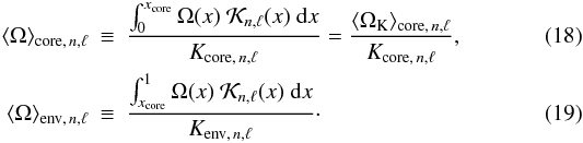We then consider dipole g-m modes that have the largest rotational splittings; they coincide with the largest inertia (Dupret et al. 2009). These modes are furthest away from the nominal pure pressure dipole modes and close to the radial modes. The splittings associated with these modes do not vary with frequency, i.e. from one radial mode to the other. Hence, we retrieve the observed splittings (Eqs. (3) and (11)): $\mathit{\delta }{\mathit{\nu }}_{\mathrm{rot}}\mathrm{=}\begin{array}{}\max \end{array}(\mathit{\delta }{\mathit{\nu }}_{\mathrm{rot}}{\mathit{,n,\ell }\mathrm{=}\mathrm{1}}_{})\mathrm{=}\begin{array}{}\max \end{array}(\mathit{\delta }{\mathit{\nu }}_{\mathrm{split}})\mathit{.}$(20)As a consequence, we can drop the subscripts n,ℓ from now on. One expects, for red giants, a more rapid rotation rate in the inner layers hence  ⟨ Ω ⟩ _env/ ⟨ Ω ⟩ _core < 1 and  ≪ 1 for very fast rotating cores (Goupil et al. 2012). For the g-m modes, numerical calculations show that K_env/K_core ≪ 1 (Fig. 8), hence α_rot ≪ 1. Thus, from Eqs. (14) and (18): 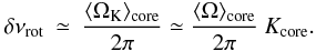$\begin{array}{ccc}\mathit{\delta }{\mathit{\nu }}_{\mathrm{rot}}& \mathrm{\simeq }& \end{array}$(21)For these modes, the displacement is essentially horizontal in the core, therefore ξ_r ≪ ξ_h. We also have I ≃ I_core, so that, from Eqs. (9) and (10), one can derive that the core kernel reduces to about 1/2, in agreement with the Ledoux coefficient of g modes (Ledoux 1951). Finally, we have 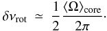$\begin{array}{ccc}\mathit{\delta }{\mathit{\nu }}_{\mathrm{rot}}& \mathrm{\simeq }& \frac{\mathrm{1}}{\mathrm{2}}\frac{\mathrm{⟨}\mathrm{\Omega }{\mathrm{⟩}}_{\mathrm{core}}}{\mathrm{2}\mathit{\pi }}\mathrm{·}\end{array}$(22)Hence, rotational splittings of g-dominated modes provide a measure of the rotation averaged over the central region. The averaged rotation roughly corresponds to the value of the rotation at the radius where the mode amplitude of the horizontal displacement ξ_h is maximum. This happens away from the center, in a core region where the rotation can have significantly decreased compared to the central rotation. In that case, the average rotation value gives a lower limit of the rotation of the very deep layers. If the rotation happens to be nearly solid in the central region, then the average rotation gives the rotation of the nearly uniformly rotating core.

Keeping in mind these limits, δν_rot can be considered as a proxy of the mean rotation period of the core  ⟨ T_rot ⟩ _c, i.e. 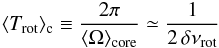$\mathrm{⟨}{\mathit{T}}_{\mathrm{rot}}{\mathrm{⟩}}_{\mathrm{c}}\mathrm{\equiv }\frac{\mathrm{2}\mathit{\pi }}{\mathrm{⟨}\mathrm{\Omega }{\mathrm{⟩}}_{\mathrm{core}}}\mathrm{\simeq }\frac{\mathrm{1}}{\mathrm{2}\hspace{0.17em}\mathit{\delta }{\mathit{\nu }}_{\mathrm{rot}}}$(23)for dipole mixed modes.

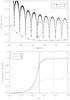Fig. 8 Top: mode inertia for radial and dipole modes of a 1 M⊙ RGB star at the bump. The evolution model has been calculated with CESAM (Morel 1997) and the oscillation frequencies were obtained with ADIPLS (Christensen-Dalsgaard 2011). Bottom: normalized integrated rotational kernels of three dipole modes: M1 and M2 are g-m modes, whereas M3 is a p-m mode. The vertical triple-dot-dashed line indicates the mean location of the hydrogen-burning shell, and the vertical dashed line indicates the base of the convective envelope.

5.2. Information from the kernels

With the CESAM code for stellar evolution (Morel 1997) and the ADIPLS code for adiabatic oscillations (Christensen-Dalsgaard 2011), we estimate the kernels in red giant models at different evolutionary states. Figure 8 shows the normalized integrated rotational kernels ${{}^{\mathrm{\int }}}_{\mathrm{0}}^{\mathit{r}}\mathrm{𝒦}\mathrm{\left(}\mathit{r}\mathrm{\right)}\hspace{0.17em}\mathrm{d}\mathit{r}\mathit{/}{{}^{\mathrm{\int }}}_{\mathrm{0}}^{\mathit{R}}\mathrm{𝒦}\mathrm{\left(}\mathit{r}\mathrm{\right)}\hspace{0.17em}\mathrm{d}\mathit{r}$ derived for a p-m mode and two g-m modes in an RGB star at the bump, with Δν ≃ 5 μHz. We verify that the kernels in g-m modes are dominated by the core, since the normalized integrated kernels reach a value larger than 0.95 at the core boundary.

These integrated kernels allow us to derive a refined estimate of the core rotation. With a 2-layer model presented in Appendix B.1, a small correction to Eq. (23) can be introduced by a factor η (Eq. (B.3)) $\mathrm{⟨}{\mathit{T}}_{\mathrm{rot}}{\mathrm{⟩}}_{\mathrm{c}}\mathrm{=}\frac{\mathrm{1}}{\mathrm{2}\hspace{0.17em}\mathit{\eta }\hspace{0.17em}\mathit{\delta }{\mathit{\nu }}_{\mathrm{rot}}}\mathrm{·}$(24)The correction factor η, slightly larger than unity, accounts for the propagation of the oscillation in the envelope. This correction is intended to provide a more accurate result than the proxy provided by Eq. (23). Values of η can be calculated for RGB stars at different evolution stages (Appendix B.1). They show that δν_rot is less dominated by the core rotation for early RGB stars compared to more evolved stages.

As the value of η results from a balance between the contributions of p and g modes, we can assume that its value depends on the mean pressure and gravity radial orders. We therefore propose a phenomenological proxy of the parameter η, justified by a simple model presented in Appendix B.2, as a function of global seismic parameters. The analysis of the integrated kernels calculated for red giant models at different evolutionary stages provides the fit $\mathit{\eta }\mathrm{\simeq }\mathrm{1}\mathrm{+}\mathit{\gamma }\frac{{\mathit{\nu }}_{\max }^{\mathrm{2}}\mathrm{\Delta }{\mathrm{\Pi }}_{\mathrm{1}}}{\mathrm{\Delta }\mathit{\nu }}\mathit{,}$(25)where ΔΠ₁ is the period spacing of gravity modes derived from the fit of the mixed modes and γ ≃ 0.65 (see Appendix B.2). The model indicates that the coefficient η decreases towards unity when a star evolves along the RGB, due to the significant increase of the gravity radial orders (Mosser et al. 2012c). The model, based on RGB stars, is assumed to be valid also for clump stars, since it only relies on global properties of the oscillation eigenfunction.

In all cases, the maximal splitting of g-m modes is highly dominated by the core rotation, and its measure is close to the core rotation. Furthermore, as found by Beck et al. (2012) and Deheuvels et al. (2012a), we note that there is no immediate link between the minimum splitting (1 − λ) δν_rot of p-m modes (Eq. (4)) and the surface rotation. The minimum splitting measured for p-m modes is still strongly dominated by the core rotation. Extracting the surface rotation, which is supposed to be small, requires a very accurate description of the kernels, which is out of the scope of this work dedicated to ensemble asteroseismology.

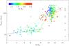Fig. 9 Mean period of core rotation as a function of the asteroseismic stellar radius, in log-log scale. Same symbols and color code as in Fig. 6. The dotted line indicates a rotation period varying as R2. The dashed (dot-dashed, triple-dot-dashed) line indicates the fit of RGB (clump, secondary clump) core rotation period. The rectangles in the right side indicate the typical error boxes, as a function of the rotation period.

6. Discussion

The relation between the maximum rotational splitting and the mean core rotation period (Eq. (23)) allows us to revisit the scaling relations established in Sect. 4. We have to reiterate that Eq. (24) is based on a strong hypothesis, resulting from the linear relation between the splitting and the core rotation rate. A high radial differential rotation profile in the core, as shown by Goupil et al. (2012) and Marques et al. (2012), would invalidate the relation.

6.1. Internal angular momentum transfer

The scaling relations in Eqs. (6) and (7) can be written in terms of  ⟨ T_rot ⟩ _c rather than δν_rot. We find, for RGB and clump stars, respectively: $\begin{array}{ccc}\mathrm{⟨}{\mathit{T}}_{\mathrm{rot}}{\mathrm{⟩}}_{\mathrm{c}}\mathrm{\propto }{\mathit{R}}^{\mathrm{0.7}\hspace{0.17em}\mathrm{\pm }\hspace{0.17em}\mathrm{0.3}}& & \mathrm{\left(}\mathrm{RGB}\mathrm{\right)}\\ \mathrm{⟨}{\mathit{T}}_{\mathrm{rot}}{\mathrm{⟩}}_{\mathrm{c}}\mathrm{\propto }{\mathit{R}}^{\mathrm{1.4}\hspace{0.17em}\mathrm{\pm }\hspace{0.17em}\mathrm{0.4}}& & \mathrm{\left(}\mathrm{clump}\mathrm{\right)}\\ \mathrm{⟨}{\mathit{T}}_{\mathrm{rot}}{\mathrm{⟩}}_{\mathrm{c}}\mathrm{\propto }{\mathit{R}}^{\mathrm{1.5}\hspace{0.17em}\mathrm{\pm }\hspace{0.17em}\mathrm{0.4}}& & \mathrm{\left(}\mathrm{2}\mathrm{ndclump}\mathrm{\right)}\mathit{.}\end{array}$We note that the absolute values of the exponents are similar to the exponents found in Eqs. (6) and (7). This comes from the fact that the correction factor η of Eq. (25) is close to unity and does not show important variation. As a consequence, the regime seen in the rotational splitting translates into a similar regime of the mean core rotation period (Fig. 9).

6.1.1. On the RGB

On the RGB, the spinning down of the core is moderate, much smaller than a variation in R² expected in case of homologous spinning down at constant total angular momentum. Angular momentum is certainly transferred from the core to the envelope, in order to spin down the core. However, a strong differential rotation profile takes place when giants ascend the RGB (Marques et al. 2012; Goupil et al. 2012).

6.1.2. Clump stars

The extrapolation of the fit reported by Eq. (26) to a typical stellar radius at the red clump shows that cores of clump stars are rotating six times slower. This slower rotation can be partly explained by the core radius change occurring when helium fusion ignition removes the degeneracy in the core. This change, estimated to be less than 50% (Sills & Pinsonneault 2000), can however not be responsible for an increase of the mean core rotation period as large as a factor of six. As a consequence, the slower rotation observed in clump stars indicates that internal angular momentum has been transferred from the rapidly rotating core to the slowly rotating envelope (Fig. 9).

6.1.3. Comparison with modeling

The comparison with modeling reinforces this view (Fig. 1 of Sills & Pinsonneault 2000). Their evolution model assumes a local conservation of angular momentum in radiative regions and solid-body rotation in convective regions. It provides values for the core rotation in a 0.8 M_⊙ star of about 50 days on the main sequence, about 2 days on the RGB at the position of maximum convection zone depth in mass, and about 7 days in the clump. This means that, even in a case where the initial rotation on the main-sequence is slow (certainly much slower than the main-sequence progenitors of the red giants studied here) and where angular momentum is massively transferred in order to insure that convective regions rotate rigidly, the predicted core rotation periods are much smaller than observed. The expansion of the convective envelope provides favorable conditions for internal gravity waves to transfer internal momentum from the core to the envelope to spin down the core rotation (Zahn et al. 1997; Mathis 2009). Talon & Charbonnel (2008) have shown that the conditions are favorable for these waves to operate at the end of the subgiant branch and during the early-AGB phase. There is observational evidence that the spinning down should have been boosted in the upper RGB too.

The comparison of the core rotation evolution on the RGB and in the clump shows that the angular momentum transfer is not enough for erasing the differential rotation in clump stars. The line representing an evolution of  ⟨ T_rot ⟩ _c with R² extrapolated to typical main-sequence stellar radii gives a much more rapid core rotation than the extrapolation from the RGB fit. This indicates that the interior structure of a red-clump star has to sustain, despite the spinning down of the core rotation, a significant differential rotation. This conclusion, implicitly based on the assumption of total angular momentum conservation, is reinforced in case of total spinning down at the tip of the RGB. However, the large similarities of the values of the core rotation period observed in clump stars, together with an evolution of  ⟨ T_rot ⟩ _c close to R² (Eq. (27)), should imply that a regime is found with a core rotation of clump stars much more rapid than the envelope rotation but closely linked to it.

6.2. Mass dependence

We have calculated, for different mass ranges  [M₁,M₂] , a mean core rotation period defined by $\mathrm{⟨}\mathrm{⟨}{\mathit{T}}_{\mathrm{rot}}{\mathrm{⟩}}_{\mathrm{c}}{\mathrm{⟩}}_{\mathrm{\left[}{\mathit{M}}_{\mathrm{1}}\mathit{,}{\mathit{M}}_{\mathrm{2}}\mathrm{\right]}}\mathrm{=}\frac{{\sum }_{{\mathit{M}}_{\mathrm{1}}}^{{\mathit{M}}_{\mathrm{2}}}\mathrm{⟨}{\mathit{T}}_{\mathrm{rot}}{\mathrm{⟩}}_{\mathrm{c}}{\mathit{R}}^{\mathrm{-}\mathit{r}}}{{\sum }_{{\mathit{M}}_{\mathrm{1}}}^{{\mathit{M}}_{\mathrm{2}}}{\mathit{R}}^{\mathrm{-}\mathit{r}}}$(29)where r is the exponent given by Eqs. (26) or (27), depending on the evolutionary status.

This expression allows us to derive a mean value even for RGB stars, in the mass range [1.2, 1.5 M_⊙] where the RGB star sample can be considered as unbiased. We do not detect any mass dependence. The situation changes drastically for clump stars, with a clear mass dependence: the mean value of  ⟨ T_rot ⟩ _c is divided by a factor of about 1.7 from 1 to 2 M_⊙. This reinforces the view that angular momentum is certainly exchanged in the upper RGB, since it may indicate a link between the amount of specific angular momentum transferred and the evolution time: high-mass red giants evolve more rapidly than lower mass stars, loose less mass, and keep a more rapidly rotating core after the tip.

7. Conclusion

Rotational splittings were measured in about 300 red giants observed during more than two years with Kepler. As first measured by Beck et al. (2012) for three red giants in the early stages of the RGB, a strong differential rotation is noted for all these red giants.

We have first shown that the rotational splitting pattern, modelled as a function of the mode frequency, is largely independent of the stellar evolution. The empirical pattern found by Mosser et al. (2012b) has been used and verified in a large set of stars and has proven to be very efficient for analysing the splittings. Independent of any modeling, we have shown that the scaling relations observed for the maximum rotational splittings in RGB stars may suggest that transfer of angular momentum must occur in their interiors.

Then, assuming that the relation between the rotational splitting and the rotation rate is linear, we have shown that the measured splittings provide an estimate of a rotation period representative of the mean core rotation. We observe that this period is larger for clump stars compared to the RGB. This requires a transfer of angular momentum in the star to spin down the core. Despite the angular momentum loss expected at the tip of the RGB, the core rotates more rapidly in clump stars than expected from an evolution as the square of the radius. This indicates a strong differential rotation in clump stars as well as in RGB stars. In other words, the mechanism responsible for the redistribution of angular momentum is efficient enough to spin down the mean core rotation but with a time scale too long for reaching a solid rotation.

The indirect estimate of the specific angular momentum shows that massive red giants observed in the secondary clump have a significantly higher specific angular momentum than in the main red clump.

This ensemble asteroseismic analysis of rotation in red giants will have to be extended to subgiants, since subgiants also show mixed modes that give access to the inner rotation profile. As Kepler continues to observe, we will have access to longer observation runs. This will provide more resolved observations of the rotational splittings at low frequency, so we hope to measure the mean core rotation on the upper part of the RGB and, if mixed modes are also present, on the asymptotic giant branch. Our findings provide strong motivation for further stellar modeling including rotation.

Online material

Appendix A: How rotational splittings are fitted

A.1. Large separation and gravity mode spacing

The first step for identifying the red giant oscillation spectrum is, as for all stars showing solar-like oscillations, the correct identification of the radial mode pattern, in order to locate precisely the location of the theoretical pure dipole pressure modes. The fit of the radial modes depends mainly on the accurate determination of the large separation. According to the universal red giant oscillation pattern (Mosser et al. 2011b), the surface offset and the curvature of the ridge are functions of the large separation. In practice, small residuals due to glitches (Miglio et al. 2010) can induce a frequency offset of about, typically, Δν/50. Thus, a second free parameter, simply a frequency offset, or equivalently an offset of ε less than 0.02 (Eq. (1)), is useful for providing the best fit of the radial ridge. The location of the dipole ridge with respect to the radial ridge is given by the small separation d₀₁ (Eq. (1)), which is a function of the large separation (Mosser et al. 2011b).

The fit of the mixed-mode pattern is based on two free parameters: the period spacing ΔΠ₁ and the coupling constant q, as defined by Eq. (9) of Mosser et al. (2012c), which closely follows the formalism of mixed modes given by Unno et al. (1989). In order to determine ΔΠ₁ on the RGB, it is worthwhile to consider that this period is a function of the large separation. For the low-mass stars of the RGB with a degenerate helium core, a convenient proxy is given by the polynomial development $\mathrm{\Delta }{\mathrm{\Pi }}_{\mathrm{1}}\mathrm{=}\mathrm{62.5}\mathrm{+}\mathrm{1.40}\hspace{0.17em}\mathrm{\Delta }\mathit{\nu }\mathrm{+}\mathrm{0.081}\hspace{0.17em}\mathrm{\Delta }{\mathit{\nu }}^{\mathrm{2}}$(A.1)with Δν in μHz and ΔΠ₁ in s, according to Fig. 3 of Mosser et al. (2012c). When the rotational splitting is larger than half the mixed mode spacing at ν_max, this step cannot be done independent of the next one.

Fig. A.1 Fit of rotational splittings, for the RGB star KIC 6144777, with an échelle diagram as a function of the reduced frequency ν/Δν − (np + ε). The radial orders are indicated on the y-axis. Radial modes (highlighted in red) are centered on 0, quadrupole modes (highlighted in green), near  − 0.12 (with a radial order np − 1), and ℓ = 3 modes, sometimes observed, (highlighted in hell blue) near 0.20. Rotational splittings are identified with the frequency of the m = 0 component given by the asymptotic relation of mixed modes, in μHz. The fit is based on peaks showing a height larger than eight times the mean background value (grey dashed lines). In order to enhance the appearance of the multiplets, highest peaks have been truncated; to enhance the short-lived radial and quadrupole modes, a smoothed spectrum is also shown, superimposed on the corresponding peaks.

Fig. A.2 Same as Fig. A.1, for the RGB star 5858947. In such a spectrum where the total splitting 2δνrot is equal to half the mixed-mode spacing at νmax, the fit allows to correctly identify the multiplets.

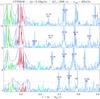Fig. A.3 Same as Fig. A.1, for the clump star KIC 4770846. The apparent low quality of the fit for p-m modes at large frequency is due to their short lifetimes (Baudin et al. 2011).

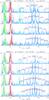Fig. A.4 Same as Fig. A.1, for the RGB stars KIC 9267654 and KIC 10866415, where the total splitting 2δνrot is nearly equal to the mixed-mode spacing at νmax. Apparent narrow multiplets are artifacts due to close combinations between components of different mixed-modes radial orders.

A.2. Rotational splittings

Great care must be taken to disentangle the splittings from the mixed mode spacings. Three major cases have to be considered for fitting the rotational splittings.

• If splittings are small and almost uniform with frequency, exceptthe modulation depicted by ℛ (Eq. (4)), then the estimate is straightforward. The unknown stellar inclination can be derived from the mode visibility, which depends on the azimuthal order m. According to the probability of having an inclination i proportional to sini, in most cases doublets with m = ± 1 are observed. Note that, even if the components m = −1 and  + 1 have the same visibility, they may in practice present different heights, due to the stochastic excitation of the modes. Such splittings smaller than the mixed-mode spacings are seen in the lower stages of the RGB and in the clump (Fig. A.1).

• If apparent splittings at ν_max seem to increase with increasing frequency, then the most plausible solution is that δν_rot is close to half the mixed-mode spacing at ν_max. These apparent splittings result in fact from a mixing of the splittings embedded with the spacings. Such a situation occurs when the apparent splittings are composed of the m = ± 1 component of the mixed mode order n_m and of the m = ∓ 1 component of the adjacent orders n_m ± 1. The true splittings, significantly larger than the apparent splittings, are almost uniform for g-m modes. This uniformity is used for iterating the solution. Such cases occur most often for RGB stars with Δν in the range [9–12 μHz] (Fig. A.4).

• If apparent splittings seem very irregular, then the most plausible solution is that δν_rot is much larger than half the mixed-mode spacing at ν_max. In fact, the apparent splittings are complex structures resulting from a mixing of components of two or three different mixed-mode orders. A careful visual inspection is necessary to disentangle them. The mixed-mode asymptotic expression and the empirical expression of the rotational splitting are accurate enough for resolving complex cases that occur for RGB stars with Δν ≤ 9 μHz (Fig. A.5).

We have used gravity échelle diagrams to represent the mixed modes (Bedding et al. 2011; Mosser et al. 2012c). Due to the complexity of the features caused by embedded splittings and mixed modes spacings, the échelle diagrams cannot be used to identify the rotational splittings, but are useful for improving the accuracy of the fit. In the examples shown (Fig. A.6), a 10-s shift between the periods of the observed and modeled peaks correspond to an accuracy in frequency of about Δν/100.

A.3. A dipole mode forest?

The complete fit of the rotational splittings is based on three parameters: the maximum splitting δν_rot and the two parameters λ and β entering the definition of ℛ. The best fit is provided by correlating the observed multiplets with synthetic multiplets.

Since the parameters λ and β are found to vary in narrow ranges, the solution for inferring δν_rot (and simultaneously ΔΠ₁ on the RGB with low Δν) is based on considering them as constants. As a result, five free parameters are enough for fitting the whole red giant oscillation spectrum. Variation of λ and β allows a better fit. The stellar inclination can be derived from the ratio of the visibility of the m = ± 1 components compared to the central component.

In a typical spectrum, more than 30 mixed-mode orders, representing about 60 to 120 individual modes with a height larger than eight times the background are simultaneously fitted. The typical accuracy of the fit, of about Δν/200 or better, is enough for avoiding any confusion in almost all cases, except for the most evolved RGB stars.

Finally, with the identification of the mixed mode spacings and of the rotational splittings, the dipole mode forest becomes a well-organized garden à la française.

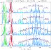Fig. A.5 Same as Fig. A.4, for the RGB star KIC 11550492. The non-negligible amplitudes of the m = 0 components complicate the analysis.

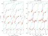Fig. A.6 Gravity échelle diagrams of the two RGB stars KIC 5858947 and 11550492. The x-axis is the period 1/ν modulo the gravity spacing ΔΠ1; for clarity, the range has been extended from  − 0.5 to 1.5 ΔΠ1. The size of the selected observed mixed modes (red diamonds) indicates their height. Plusses give the expected location of the mixed modes, with m = −1 in light blue, m = 0 in green and m = +1 in dark blue.

Appendix B: Two-layer model

B.1. Core and surface contributions

In order to estimate the contribution of the core and surface rotation, we simplify the stellar stratification to a 2-layer model. We denote by δν_c and δν_s the rotational frequency of the core and at the surface, respectively, and δν_g/2 and δν_p the measured splitting on g and p modes, respectively. The factor 1/2 in δν_g/2 accounts for the Ledoux coefficient. The contributions of the surface and of the core are written 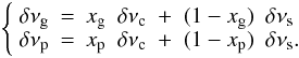$\{\begin{array}{c}\\ \mathit{\delta }{\mathit{\nu }}_{\mathrm{g}}& \mathrm{=}& {\mathit{x}}_{\mathrm{g}}& \mathit{\delta }{\mathit{\nu }}_{\mathrm{c}}& \mathrm{+}& \mathrm{(}\mathrm{1}\mathrm{-}{\mathit{x}}_{\mathrm{g}}\mathrm{)}& \mathit{\delta }{\mathit{\nu }}_{\mathrm{s}}\\ \mathit{\delta }{\mathit{\nu }}_{\mathrm{p}}& \mathrm{=}& {\mathit{x}}_{\mathrm{p}}& \mathit{\delta }{\mathit{\nu }}_{\mathrm{c}}& \mathrm{+}& \mathrm{(}\mathrm{1}\mathrm{-}{\mathit{x}}_{\mathrm{p}}\mathrm{)}& \mathit{\delta }{\mathit{\nu }}_{\mathrm{s}}\mathit{.}\end{array}$(B.1)The coefficient x_p and x_g are derived from the rotational kernels. From the solution 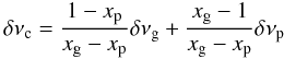$\mathit{\delta }{\mathit{\nu }}_{\mathrm{c}}\mathrm{=}\frac{\mathrm{1}\mathrm{-}{\mathit{x}}_{\mathrm{p}}}{{\mathit{x}}_{\mathrm{g}}\mathrm{-}{\mathit{x}}_{\mathrm{p}}}\mathit{\delta }{\mathit{\nu }}_{\mathrm{g}}\mathrm{+}\frac{{\mathit{x}}_{\mathrm{g}}\mathrm{-}\mathrm{1}}{{\mathit{x}}_{\mathrm{g}}\mathrm{-}{\mathit{x}}_{\mathrm{p}}}\mathit{\delta }{\mathit{\nu }}_{\mathrm{p}}$(B.2)and from the observation of the splitting of p-m modes indicating δν_p ≃ δν_g/4 (a factor of about 1/2 comes from 1 − λ in Eq. (4), an another factor of 1/2 comes from the Ledoux coefficient), one derives that the measure of δν_g is an indicator of the core rotation 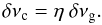$\mathit{\delta }{\mathit{\nu }}_{\mathrm{c}}\mathrm{=}\mathit{\eta }\mathit{\delta }{\mathit{\nu }}_{\mathrm{g}}\mathit{.}$(B.3)For an RGB star at the bump with Δν = 5 μHz, the values x_p and x_g derived from the kernels give η = 1.06 ± 0.04, very close to unity. A less evolved star, as considered by Beck et al. (2012), whose mixed modes correspond to much smaller radial gravity orders, has $\mathit{\eta }\mathrm{=}\mathrm{1.4}{\mathrm{5}}_{-0.15}^{\mathrm{+}\mathrm{0.30}}$. Deheuvels et al. (2012a) derived a similar result for a giant with Δν ≃ 29 μHz at the bottom of the RGB. This shows that δν_rot is less dominated by the core rotation for early RGB stars. One also derives that, in all cases, the surface rotation δν_s is small, and that measuring it precisely from the g-m mode-splitting is not possible.

B.2. Link to the eigenfunction properties

The value of the coefficients x_g and x_p introduced in Eq. (B.1) can be approximated by the expression of the rotational splitting (Eqs. (8) and (9)). Basically, the integration of the wave function has a contribution varying as the number of nodes in the core and in the envelope, respectively. As a consequence, x_g ∝ n_g and x_p ∝ n_p. In order to more precisely account for the complex form of the wave function, we suppose: 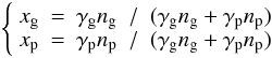$\{\begin{array}{c}\\ {\mathit{x}}_{\mathrm{g}}& \mathrm{=}& {\mathit{\gamma }}_{\mathrm{g}}{\mathit{n}}_{\mathrm{g}}& \mathit{/}& \mathrm{(}{\mathit{\gamma }}_{\mathrm{g}}{\mathit{n}}_{\mathrm{g}}\mathrm{+}{\mathit{\gamma }}_{\mathrm{p}}{\mathit{n}}_{\mathrm{p}}\mathrm{)}\\ {\mathit{x}}_{\mathrm{p}}& \mathrm{=}& {\mathit{\gamma }}_{\mathrm{p}}{\mathit{n}}_{\mathrm{p}}& \mathit{/}& \mathrm{(}{\mathit{\gamma }}_{\mathrm{g}}{\mathit{n}}_{\mathrm{g}}\mathrm{+}{\mathit{\gamma }}_{\mathrm{p}}{\mathit{n}}_{\mathrm{p}}\mathrm{)}\end{array}$(B.4)\newpage\noindentwith γ_g < 0 to account for the negative value of n_g. The validity of this development implicitly assumes that γ_p and  | γ_g |  are constant not so far from unity. Hence, neglecting δν_s in Eq. (B.1), we derive: $\mathit{\delta }{\mathit{\nu }}_{\mathrm{c}}\mathrm{\simeq }\left[\mathrm{1}\mathrm{+}\frac{{\mathit{\gamma }}_{\mathrm{p}}}{{\mathit{\gamma }}_{\mathrm{g}}}\frac{{\mathit{n}}_{\mathrm{p}}}{{\mathit{n}}_{\mathrm{g}}}\right]\mathit{\delta }{\mathit{\nu }}_{\mathrm{g}}\mathrm{\simeq }\left[\mathrm{1}\mathrm{-}\mathit{\gamma }\frac{{\mathit{n}}_{\mathrm{p}}}{{\mathit{n}}_{\mathrm{g}}}\right]\mathit{\delta }{\mathit{\nu }}_{\mathrm{g}}\mathit{.}$(B.5)The radial order n_p and n_g have to be estimated at the frequency ν_max where the oscillation amplitude is maximum. Then, we can derive that η = δν_c/δν_g is related to the global seismic parameters Δν and ΔΠ₁, where ΔΠ₁ is the period spacing of gravity modes: $\mathit{\eta }\mathrm{\simeq }\mathrm{1}\mathrm{+}\mathit{\gamma }\frac{{\mathit{\nu }}_{\max }^{\mathrm{2}}\mathrm{\Delta }{\mathrm{\Pi }}_{\mathrm{1}}}{\mathrm{\Delta }\mathit{\nu }}\mathrm{·}$(B.6)The fit of the integrated kernels calculated at different evolutionary stages gives γ ≃ 0.65. This phenomenological result based on a simple two-layer model is to be considered as a proxy only.

Acknowledgments

Funding for this Discovery mission is provided by NASA’s Science Mission Directorate. This work partially used data analyzed under the NASA grant NNX12AE17G. NCAR is supported by the National Science Foundation. P.G.B. has received funding from the European Research Council under the European Community’s Seventh Framework Programme (FP7/2007-2013)/ERC grant agreement No. PROSPERITY. SH acknowledges financial support from the Netherlands Organisation for Scientific research (NWO). Y.E. acknowledges financial support from the UK STFC. R.A.G. acknowledges the support of the European Communitys Seventh Framework Program (FP7/2007-2013) under grant agreement No. 269194 (IRSES/ASK).

References

All Tables

All Figures

Fig. 1 Échelle diagram of a typical RGB star (KIC 6144777) as a function of ν/Δν − (np + ε). The radial order np is indicated on the y-axis. Radial modes (highlighted in red) are centered on 0, quadrupole modes (highlighted in green), near − 0.12 (with a radial order np − 1), and ℓ = 3 modes, sometimes observed, (highlighted in light blue) near 0.20. Dipole mixed modes are identified with the frequency given by the asymptotic relation of mixed modes, in μHz. The fit is based on peaks showing a height larger than eight times the mean background value (grey dashed lines).

In the text

	Fig. 2 Empirical rotation profile ℛnp for dipole mixed modes associated to the pure p mode of radial order np, as a function of the reduced frequency ν/Δν − (np + ε).
In the text

	Fig. 3 Zoom on the oscillation spectrum of the target KIC 10777816. Different narrow filters centered in the ℓ = 1 mixed mode range, indicated with different line styles, allow us to measure a local rotational splitting in each filter. For clarity, only those filters centered on possible multiplets have been represented.
In the text

	Fig. 4 Comparison of the splittings measured with the EACF automated method to the splittings measured with the fit of the mixed modes (Eq. (4)). Red asterisks correspond to rotational splittings too large to be accurately measured in an automated way and hence excluded from the sample.
In the text

	Fig. 5 Zoom on the rotational splittings of the mixed modes corresponding to the radial orders np = 8 → 11 in the giant KIC 9574650, in an échelle diagram as a function of the reduced frequency ν/Δν − (np + ε). All triplets (m = −1,0,1) are identified with the function ℛ defined by Eq. (4). At low frequency, multiplets are overlapping.
In the text

Fig. 6 Rotational splitting δνrot as a function of the large separation Δν, in log-log scale. The dotted line indicates the frequency resolution. The dashed and dot-dashed lines represent the confusion limit with mixed modes in RGB and clump stars, respectively, derived from Mosser et al. (2012c). Crosses correspond to RGB stars, triangles to clump stars, and squares to secondary clump stars. The color code gives the mass estimated from the asteroseismic global parameters. The vertical bars indicate the mean error bars, as a function of the rotational splitting.

In the text

	Fig. 7 Rotation splitting δνrot as a function of the asteroseismic stellar radius, in log-log scale. Same symbols and color code as in Fig. 6. The dotted line indicates a splitting varying as R-2. The dashed (dot-dashed, triple-dot-dashed) line corresponds to the fit of RGB (clump, secondary clump) splittings.
In the text

Fig. 8 Top: mode inertia for radial and dipole modes of a 1 M⊙ RGB star at the bump. The evolution model has been calculated with CESAM (Morel 1997) and the oscillation frequencies were obtained with ADIPLS (Christensen-Dalsgaard 2011). Bottom: normalized integrated rotational kernels of three dipole modes: M1 and M2 are g-m modes, whereas M3 is a p-m mode. The vertical triple-dot-dashed line indicates the mean location of the hydrogen-burning shell, and the vertical dashed line indicates the base of the convective envelope.

In the text

Fig. 9 Mean period of core rotation as a function of the asteroseismic stellar radius, in log-log scale. Same symbols and color code as in Fig. 6. The dotted line indicates a rotation period varying as R2. The dashed (dot-dashed, triple-dot-dashed) line indicates the fit of RGB (clump, secondary clump) core rotation period. The rectangles in the right side indicate the typical error boxes, as a function of the rotation period.

In the text

Fig. A.1 Fit of rotational splittings, for the RGB star KIC 6144777, with an échelle diagram as a function of the reduced frequency ν/Δν − (np + ε). The radial orders are indicated on the y-axis. Radial modes (highlighted in red) are centered on 0, quadrupole modes (highlighted in green), near  − 0.12 (with a radial order np − 1), and ℓ = 3 modes, sometimes observed, (highlighted in hell blue) near 0.20. Rotational splittings are identified with the frequency of the m = 0 component given by the asymptotic relation of mixed modes, in μHz. The fit is based on peaks showing a height larger than eight times the mean background value (grey dashed lines). In order to enhance the appearance of the multiplets, highest peaks have been truncated; to enhance the short-lived radial and quadrupole modes, a smoothed spectrum is also shown, superimposed on the corresponding peaks.

In the text

	Fig. A.2 Same as Fig. A.1, for the RGB star 5858947. In such a spectrum where the total splitting 2δνrot is equal to half the mixed-mode spacing at νmax, the fit allows to correctly identify the multiplets.
In the text

	Fig. A.3 Same as Fig. A.1, for the clump star KIC 4770846. The apparent low quality of the fit for p-m modes at large frequency is due to their short lifetimes (Baudin et al. 2011).
In the text

	Fig. A.4 Same as Fig. A.1, for the RGB stars KIC 9267654 and KIC 10866415, where the total splitting 2δνrot is nearly equal to the mixed-mode spacing at νmax. Apparent narrow multiplets are artifacts due to close combinations between components of different mixed-modes radial orders.
In the text

	Fig. A.5 Same as Fig. A.4, for the RGB star KIC 11550492. The non-negligible amplitudes of the m = 0 components complicate the analysis.
In the text

Fig. A.6 Gravity échelle diagrams of the two RGB stars KIC 5858947 and 11550492. The x-axis is the period 1/ν modulo the gravity spacing ΔΠ1; for clarity, the range has been extended from  − 0.5 to 1.5 ΔΠ1. The size of the selected observed mixed modes (red diamonds) indicates their height. Plusses give the expected location of the mixed modes, with m = −1 in light blue, m = 0 in green and m = +1 in dark blue.

In the text

References

- Baudin, F., Barban, C., Belkacem, K., et al. 2011, A&A, 529, A84 [NASA ADS] [CrossRef] [EDP Sciences] [Google Scholar]
- Beck, P. G., Bedding, T. R., Mosser, B., et al. 2011, Science, 332, 205 [NASA ADS] [CrossRef] [PubMed] [Google Scholar]
- Beck, P. G., Montalban, J., Kallinger, T., et al. 2012, Nature, 481, 55 [NASA ADS] [CrossRef] [Google Scholar]
- Bedding, T. R., Huber, D., Stello, D., et al. 2010, ApJ, 713, L176 [NASA ADS] [CrossRef] [Google Scholar]
- Bedding, T. R., Mosser, B., Huber, D., et al. 2011, Nature, 471, 608 [NASA ADS] [CrossRef] [PubMed] [Google Scholar]
- Borucki, W. J., Koch, D., Basri, G., et al. 2010, Science, 327, 977 [NASA ADS] [CrossRef] [PubMed] [Google Scholar]
- Brown, T. M., Latham, D. W., Everett, M. E., & Esquerdo, G. A. 2011, AJ, 142, 112 [NASA ADS] [CrossRef] [Google Scholar]
- Brun, A. S., & Palacios, A. 2009, ApJ, 702, 1078 [NASA ADS] [CrossRef] [Google Scholar]
- Canto Martins, B. L., Lèbre, A., Palacios, A., et al. 2011, A&A, 527, A94 [NASA ADS] [CrossRef] [EDP Sciences] [Google Scholar]
- Carney, B. W., Gray, D. F., Yong, D., et al. 2008, AJ, 135, 892 [NASA ADS] [CrossRef] [Google Scholar]
- Charbonnel, C., & Talon, S. 2005, Science, 309, 2189 [NASA ADS] [CrossRef] [PubMed] [Google Scholar]
- Christensen-Dalsgaard, J. 2011, in Astrophysics Source Code Library, record ascl:1109.002, 9002 [Google Scholar]
- Christensen-Dalsgaard, J., & Berthomieu, G. 1991, Theory of solar oscillations, eds. A. N. Cox, W. C. Livingston, & M. S. Matthews (Tucson, AZ: University of Arizona Press), 401 [Google Scholar]
- Christensen-Dalsgaard, J., & Frandsen, S. 1983, Sol. Phys., 82, 469 [Google Scholar]
- Corsaro, E., Stello, D., Huber, D., et al. 2012, ApJ, 757, 190 [NASA ADS] [CrossRef] [Google Scholar]
- De Ridder, J., Barban, C., Baudin, F., et al. 2009, Nature, 459, 398 [Google Scholar]
- Deheuvels, S., García, R. A., Chaplin, W. J., et al. 2012a, ApJ, 756, 19 [NASA ADS] [CrossRef] [Google Scholar]
- Deheuvels, S., Ouazzani, R., & Basu. 2012b, A&A, submitted [Google Scholar]
- Dupret, M., Belkacem, K., Samadi, R., et al. 2009, A&A, 506, 57 [NASA ADS] [CrossRef] [EDP Sciences] [Google Scholar]
- Dziembowski, W. A., Gough, D. O., Houdek, G., & Sienkiewicz, R. 2001, MNRAS, 328, 601 [NASA ADS] [CrossRef] [Google Scholar]
- Eggenberger, P., Montalbán, J., & Miglio, A. 2012, A&A, 544, L4 [NASA ADS] [CrossRef] [EDP Sciences] [Google Scholar]
- García, R. A., Hekker, S., Stello, D., et al. 2011, MNRAS, 414, L6 [NASA ADS] [CrossRef] [Google Scholar]
- Goupil, M., Mosser, B., Marques, J., et al. 2012, A&A, submitted [Google Scholar]
- Goupil, M. J. 2009, in The Rotation of Sun and Stars, Lect. Notes Phys. (Berlin: Springer Verlag), 765, 45 [NASA ADS] [CrossRef] [Google Scholar]
- Hekker, S., Kallinger, T., Baudin, F., et al. 2009, A&A, 506, 465 [NASA ADS] [CrossRef] [EDP Sciences] [Google Scholar]
- Hekker, S., Elsworth, Y., De Ridder, J., et al. 2011, A&A, 525, A131 [NASA ADS] [CrossRef] [EDP Sciences] [Google Scholar]
- Hekker, S., Elsworth, Y., Mosser, B., et al. 2012, A&A, 544, A90 [NASA ADS] [CrossRef] [EDP Sciences] [Google Scholar]
- Huber, D., Bedding, T. R., Stello, D., et al. 2010, ApJ, 723, 1607 [NASA ADS] [CrossRef] [Google Scholar]
- Huber, D., Bedding, T. R., Stello, D., et al. 2011, ApJ, 743, 143 [NASA ADS] [CrossRef] [Google Scholar]
- Iben, I. Jr. 1971, PASP, 83, 697 [NASA ADS] [CrossRef] [Google Scholar]
- Jenkins, J. M., Caldwell, D. A., Chandrasekaran, H., et al. 2010, ApJ, 713, L87 [NASA ADS] [CrossRef] [Google Scholar]
- Kallinger, T., Mosser, B., Hekker, S., et al. 2010, A&A, 522, A1 [NASA ADS] [CrossRef] [EDP Sciences] [Google Scholar]
- Kallinger, T., Hekker, S., Mosser, B., et al. 2012, A&A, 541, A51 [NASA ADS] [CrossRef] [EDP Sciences] [Google Scholar]
- Kawaler, S. D., Sekii, T., & Gough, D. 1999, ApJ, 516, 349 [NASA ADS] [CrossRef] [Google Scholar]
- Lagarde, N., Decressin, T., Charbonnel, C., et al. 2012, A&A, 543, A108 [NASA ADS] [CrossRef] [EDP Sciences] [Google Scholar]
- Ledoux, P. 1951, ApJ, 114, 373 [NASA ADS] [CrossRef] [Google Scholar]
- Maeder, A. 2009, Physics, Formation and Evolution of Rotating Stars (Berlin Heidelberg: Springer) [Google Scholar]
- Marques, J., Goupil, M., Lebreton, Y., et al. 2012, A&A, accepted [Google Scholar]
- Mathis, S. 2009, A&A, 506, 811 [NASA ADS] [CrossRef] [EDP Sciences] [Google Scholar]
- Miglio, A., Montalbán, J., Baudin, F., et al. 2009, A&A, 503, L21 [NASA ADS] [CrossRef] [EDP Sciences] [MathSciNet] [Google Scholar]
- Miglio, A., Montalbán, J., Carrier, F., et al. 2010, A&A, 520, L6 [NASA ADS] [CrossRef] [EDP Sciences] [Google Scholar]
- Morel, P. 1997, A&AS, 124, 597 [NASA ADS] [CrossRef] [EDP Sciences] [MathSciNet] [PubMed] [Google Scholar]
- Mosser, B. 2010, Astron. Nachr., 331, 944 [Google Scholar]
- Mosser, B., & Appourchaux, T. 2009, A&A, 508, 877 [NASA ADS] [CrossRef] [EDP Sciences] [Google Scholar]
- Mosser, B., Belkacem, K., Goupil, M., et al. 2010, A&A, 517, A22 [NASA ADS] [CrossRef] [EDP Sciences] [Google Scholar]
- Mosser, B., Barban, C., Montalbán, J., et al. 2011a, A&A, 532, A86 [NASA ADS] [CrossRef] [EDP Sciences] [Google Scholar]
- Mosser, B., Belkacem, K., Goupil, M., et al. 2011b, A&A, 525, L9 [NASA ADS] [CrossRef] [EDP Sciences] [Google Scholar]
- Mosser, B., Michel, E., Belkacem, K., et al. 2012a, A&A, submitted [Google Scholar]
- Mosser, B., Elsworth, Y., Hekker, S., et al. 2012b, A&A, 537, A30 [NASA ADS] [CrossRef] [EDP Sciences] [Google Scholar]
- Mosser, B., Goupil, M. J., Belkacem, K., et al. 2012c, A&A, 540, A143 [NASA ADS] [CrossRef] [EDP Sciences] [Google Scholar]
- Shibahashi, H. 1979, PASJ, 31, 87 [NASA ADS] [Google Scholar]
- Sills, A., & Pinsonneault, M. H. 2000, ApJ, 540, 489 [NASA ADS] [CrossRef] [Google Scholar]
- Talon, S., & Charbonnel, C. 2008, A&A, 482, 597 [NASA ADS] [CrossRef] [EDP Sciences] [Google Scholar]
- Tassoul, M. 1980, ApJS, 43, 469 [NASA ADS] [CrossRef] [Google Scholar]
- Unno, W., Osaki, Y., Ando, H., Saio, H., & Shibahashi, H. 1989, Nonradial oscillations of stars (Tokyo: University of Tokyo Press) [Google Scholar]
- Verner, G. A., Elsworth, Y., Chaplin, W. J., et al. 2011, MNRAS, 415, 3539 [NASA ADS] [CrossRef] [Google Scholar]
- Zahn, J.-P. 1992, A&A, 265, 115 [NASA ADS] [Google Scholar]
- Zahn, J.-P., Talon, S., & Matias, J. 1997, A&A, 322, 320 [Google Scholar]