| Issue |
A&A
Volume 548, December 2012
|
|
|---|---|---|
| Article Number | A10 | |
| Number of page(s) | 14 | |
| Section | Stellar structure and evolution | |
| DOI | https://doi.org/10.1051/0004-6361/201220106 | |
| Published online | 13 November 2012 | |
Online material
Appendix A: How rotational splittings are fitted
A.1. Large separation and gravity mode spacing
The first step for identifying the red giant oscillation spectrum is, as for all stars showing solar-like oscillations, the correct identification of the radial mode pattern, in order to locate precisely the location of the theoretical pure dipole pressure modes. The fit of the radial modes depends mainly on the accurate determination of the large separation. According to the universal red giant oscillation pattern (Mosser et al. 2011b), the surface offset and the curvature of the ridge are functions of the large separation. In practice, small residuals due to glitches (Miglio et al. 2010) can induce a frequency offset of about, typically, Δν/50. Thus, a second free parameter, simply a frequency offset, or equivalently an offset of ε less than 0.02 (Eq. (1)), is useful for providing the best fit of the radial ridge. The location of the dipole ridge with respect to the radial ridge is given by the small separation d01 (Eq. (1)), which is a function of the large separation (Mosser et al. 2011b).
The fit of the mixed-mode pattern is based on two free parameters: the period spacing ΔΠ1 and the coupling constant q, as defined by Eq. (9) of Mosser et al. (2012c), which closely follows the formalism of mixed modes given by Unno et al. (1989). In order to determine ΔΠ1 on the RGB, it is worthwhile to consider that this period is a function of the large separation. For the low-mass stars of the RGB with a degenerate helium core, a convenient proxy is given by the polynomial development  (A.1)with Δν in μHz and ΔΠ1 in s, according to Fig. 3 of Mosser et al. (2012c). When the rotational splitting is larger than half the mixed mode spacing at νmax, this step cannot be done independent of the next one.
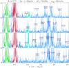 |
Fig. A.1
Fit of rotational splittings, for the RGB star KIC 6144777, with an échelle diagram as a function of the reduced frequency ν/Δν − (np + ε). The radial orders are indicated on the y-axis. Radial modes (highlighted in red) are centered on 0, quadrupole modes (highlighted in green), near − 0.12 (with a radial order np − 1), and ℓ = 3 modes, sometimes observed, (highlighted in hell blue) near 0.20. Rotational splittings are identified with the frequency of the m = 0 component given by the asymptotic relation of mixed modes, in μHz. The fit is based on peaks showing a height larger than eight times the mean background value (grey dashed lines). In order to enhance the appearance of the multiplets, highest peaks have been truncated; to enhance the short-lived radial and quadrupole modes, a smoothed spectrum is also shown, superimposed on the corresponding peaks. |
| Open with DEXTER | |
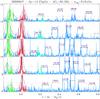 |
Fig. A.2
Same as Fig. A.1, for the RGB star 5858947. In such a spectrum where the total splitting 2δνrot is equal to half the mixed-mode spacing at νmax, the fit allows to correctly identify the multiplets. |
| Open with DEXTER | |
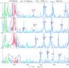 |
Fig. A.3
Same as Fig. A.1, for the clump star KIC 4770846. The apparent low quality of the fit for p-m modes at large frequency is due to their short lifetimes (Baudin et al. 2011). |
| Open with DEXTER | |
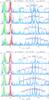 |
Fig. A.4
Same as Fig. A.1, for the RGB stars KIC 9267654 and KIC 10866415, where the total splitting 2δνrot is nearly equal to the mixed-mode spacing at νmax. Apparent narrow multiplets are artifacts due to close combinations between components of different mixed-modes radial orders. |
| Open with DEXTER | |
A.2. Rotational splittings
Great care must be taken to disentangle the splittings from the mixed mode spacings. Three major cases have to be considered for fitting the rotational splittings.
-
If splittings are small and almost uniform with frequency, exceptthe modulation depicted by ℛ (Eq. (4)), then the estimate is straightforward. The unknown stellar inclination can be derived from the mode visibility, which depends on the azimuthal order m. According to the probability of having an inclination i proportional to sini, in most cases doublets with m = ± 1 are observed. Note that, even if the components m = −1 and + 1 have the same visibility, they may in practice present different heights, due to the stochastic excitation of the modes. Such splittings smaller than the mixed-mode spacings are seen in the lower stages of the RGB and in the clump (Fig. A.1).
-
If apparent splittings at νmax seem to increase with increasing frequency, then the most plausible solution is that δνrot is close to half the mixed-mode spacing at νmax. These apparent splittings result in fact from a mixing of the splittings embedded with the spacings. Such a situation occurs when the apparent splittings are composed of the m = ± 1 component of the mixed mode order nm and of the m = ∓ 1 component of the adjacent orders nm ± 1. The true splittings, significantly larger than the apparent splittings, are almost uniform for g-m modes. This uniformity is used for iterating the solution. Such cases occur most often for RGB stars with Δν in the range [9–12 μHz] (Fig. A.4).
-
If apparent splittings seem very irregular, then the most plausible solution is that δνrot is much larger than half the mixed-mode spacing at νmax. In fact, the apparent splittings are complex structures resulting from a mixing of components of two or three different mixed-mode orders. A careful visual inspection is necessary to disentangle them. The mixed-mode asymptotic expression and the empirical expression of the rotational splitting are accurate enough for resolving complex cases that occur for RGB stars with Δν ≤ 9 μHz (Fig. A.5).
We have used gravity échelle diagrams to represent the mixed modes (Bedding et al. 2011; Mosser et al. 2012c). Due to the complexity of the features caused by embedded splittings and mixed modes spacings, the échelle diagrams cannot be used to identify the rotational splittings, but are useful for improving the accuracy of the fit. In the examples shown (Fig. A.6), a 10-s shift between the periods of the observed and modeled peaks correspond to an accuracy in frequency of about Δν/100.
A.3. A dipole mode forest?
The complete fit of the rotational splittings is based on three parameters: the maximum splitting δνrot and the two parameters λ and β entering the definition of ℛ. The best fit is provided by correlating the observed multiplets with synthetic multiplets.
Since the parameters λ and β are found to vary in narrow ranges, the solution for inferring δνrot (and simultaneously ΔΠ1 on the RGB with low Δν) is based on considering them as constants. As a result, five free parameters are enough for fitting the whole red giant oscillation spectrum. Variation of λ and β allows a better fit. The stellar inclination can be derived from the ratio of the visibility of the m = ± 1 components compared to the central component.
In a typical spectrum, more than 30 mixed-mode orders, representing about 60 to 120 individual modes with a height larger than eight times the background are simultaneously fitted. The typical accuracy of the fit, of about Δν/200 or better, is enough for avoiding any confusion in almost all cases, except for the most evolved RGB stars.
Finally, with the identification of the mixed mode spacings and of the rotational splittings, the dipole mode forest becomes a well-organized garden à la française.
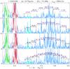 |
Fig. A.5
Same as Fig. A.4, for the RGB star KIC 11550492. The non-negligible amplitudes of the m = 0 components complicate the analysis. |
| Open with DEXTER | |
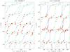 |
Fig. A.6
Gravity échelle diagrams of the two RGB stars KIC 5858947 and 11550492. The x-axis is the period 1/ν modulo the gravity spacing ΔΠ1; for clarity, the range has been extended from − 0.5 to 1.5 ΔΠ1. The size of the selected observed mixed modes (red diamonds) indicates their height. Plusses give the expected location of the mixed modes, with m = −1 in light blue, m = 0 in green and m = +1 in dark blue. |
| Open with DEXTER | |
Appendix B: Two-layer model
B.1. Core and surface contributions
In order to estimate the contribution of the core and surface rotation, we simplify the stellar stratification to a 2-layer model. We denote by δνc and δνs the rotational frequency of the core and at the surface, respectively, and δνg/2 and δνp the measured splitting on g and p modes, respectively. The factor 1/2 in δνg/2 accounts for the Ledoux coefficient. The contributions of the surface and of the core are written 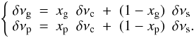 (B.1)The coefficient xp and xg are derived from the rotational kernels. From the solution
 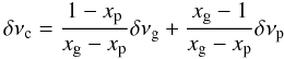 (B.2)and from the observation of the splitting of p-m modes indicating δνp ≃ δνg/4 (a factor of about 1/2 comes from 1 − λ in Eq. (4), an another factor of 1/2 comes from the Ledoux coefficient), one derives that the measure of δνg is an indicator of the core rotation
  (B.3)For an RGB star at the bump with Δν = 5 μHz, the values xp and xg derived from the kernels give η = 1.06 ± 0.04, very close to unity. A less evolved star, as considered by Beck et al. (2012), whose mixed modes correspond to much smaller radial gravity orders, has
  . Deheuvels et al. (2012a) derived a similar result for a giant with Δν ≃ 29 μHz at the bottom of the RGB. This shows that δνrot is less dominated by the core rotation for early RGB stars. One also derives that, in all cases, the surface rotation δνs is small, and that measuring it precisely from the g-m mode-splitting is not possible.
B.2. Link to the eigenfunction properties
The value of the coefficients xg and xp introduced in Eq. (B.1) can be approximated by the expression of the rotational splitting (Eqs. (8) and (9)). Basically, the integration of the wave function has a contribution varying as the number of nodes in the core and in the envelope, respectively. As a consequence, xg ∝ ng and xp ∝ np. In order to more precisely account for the complex form of the wave function, we suppose: 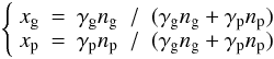 (B.4)\newpage\noindentwith γg < 0 to account for the negative value of ng. The validity of this development implicitly assumes that γp and | γg | are constant not so far from unity. Hence, neglecting δνs in Eq. (B.1), we derive:
 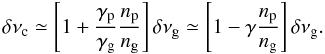 (B.5)The radial order np and ng have to be estimated at the frequency νmax where the oscillation amplitude is maximum. Then, we can derive that η = δνc/δνg is related to the global seismic parameters Δν and ΔΠ1, where ΔΠ1 is the period spacing of gravity modes:
 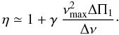 (B.6)The fit of the integrated kernels calculated at different evolutionary stages gives γ ≃ 0.65. This phenomenological result based on a simple two-layer model is to be considered as a proxy only.
© ESO, 2012
Current usage metrics show cumulative count of Article Views (full-text article views including HTML views, PDF and ePub downloads, according to the available data) and Abstracts Views on Vision4Press platform.
Data correspond to usage on the plateform after 2015. The current usage metrics is available 48-96 hours after online publication and is updated daily on week days.
Initial download of the metrics may take a while.