| Issue |
A&A
Volume 548, December 2012
|
|
|---|---|---|
| Article Number | A28 | |
| Number of page(s) | 7 | |
| Section | Astronomical instrumentation | |
| DOI | https://doi.org/10.1051/0004-6361/201219968 | |
| Published online | 14 November 2012 | |
Timing accuracy of the Swift X-Ray Telescope in WT mode
1 INAF – Istituto di Astrofisica Spaziale e Fisica Cosmica di Palermo, via U. La Malfa 153, 90146 Palermo, Italy
e-mail: cusumano@ifc.inaf.it
2 ASI Science Data Center, via G. Galilei, 00044 Frascati, Italy
3 INAF – Osservatorio Astronomico di Roma, via Frascati 33, 00040 Monteporzio Catone, Italy
4 Department of Physics and Astronomy, University of Leicester, University Road, Leicester LE1 7RH, UK
5 Department of Astronomy and Astrophysics, The Pennsylvania State University, 525 Davey Laboratory, University Park, Pennsylvania 16802, USA
6 INAF – Osservatorio Astronomico di Brera, via Bianchi 46, 23807 Merate, Italy
Received: 9 July 2012
Accepted: 14 October 2012
Context. The X-Ray Telescope (XRT) on board Swift was mainly designed to provide detailed position, timing and spectroscopic information on gamma-ray burst (GRB) afterglows. During the mission lifetime the fraction of observing time allocated to other types of source has been steadily increased.
Aims. In this paper, we report on the results of the in-flight calibration of the timing capabilities of the XRT in Windowed Timing read-out mode.
Methods. We use observations of the Crab pulsar to evaluate the accuracy of the pulse period determination by comparing the values obtained by the XRT timing analysis with the values derived from radio monitoring. We also check the absolute time reconstruction measuring the phase position of the main peak in the Crab profile and comparing it both with the value reported in literature and with the result that we obtain from a simultaneous Rossi X-Ray Timing Explorer (RXTE) observation.
Results. We find that the accuracy in period determination for the Crab pulsar is of the order of a few picoseconds for the observation with the largest data time span. The absolute time reconstruction, measured using the position of the Crab main peak, shows that the main peak anticipates the phase of the position reported in literature for RXTE by ~270 μs on average (~150 μs when data are reduced with the attitude file corrected with the UVOT data). The analysis of the simultaneous Swift-XRT and RXTE proportional counter array (PCA) observations confirms that the XRT Crab profile leads the PCA profile by ~200 μs. The analysis of XRT photodiode mode data and BAT event data shows a main peak position in good agreement with the RXTE, suggesting the discrepancy observed in XRT data in Windowed Timing mode is likely due to a systematic offset in the time assignment for this XRT read out mode.
Key words: methods: data analysis / instrumentation: detectors / pulsars: general / pulsars: individual: PSR J0534+2200
© ESO, 2012
1. Introduction
The Swift satellite (Gehrels et al. 2004), launched on 2004 Nov. 20, was mainly designed to detect and localize gamma-ray bursts (GRBs), providing autonomous rapid-response observations and long-term monitoring of the afterglow emission in a broad energy band from UV/optical to X-rays. After 7 years of operation it has observed more than 600 GRBs, collecting a huge amount of prompt and afterglow data whose study has revolutionized our understanding of the GRB phenomenology. Besides GRBs, Swift has observed many other classes of cosmic source, dedicating a growing fraction of its observing time to the so called “secondary” science.
The Swift payload includes three instruments: the Burst Alert Telescope (BAT: Barthelmy et al. 2005) observing in the 15–350 keV band, the X-Ray Telescope (XRT; Burrows et al. 2005) with an energy range of 0.3–10 keV and the Ultra-Violet/Optical Telescope (UVOT; Roming et al. 2005) with a wavelength range of 170–650 nm. XRT is a focusing X-ray telescope based on grazing incidence Wolter I mirrors, equipped with a single e2v CCD-22 detector at its focal plane. The XRT focal detector was designed to support four different data read-out modes (see Hill et al. 2004, for an exhaustive description) in order to cover a wide range of source intensities and to follow rapid variability of transient phenomena through an automatic transition among the read-out modes according to the intensity of the source. The imaging read-out mode is used soon after the slew to a newly detected transient phenomenon to record a prompt image of the field of view for a rapid evaluation of the source coordinates, with no spectroscopy or time resolved data. The photodiode mode (PD) was designed to observe very bright sources, up to 60 Crab, with no spatial information and to achieve a high timing resolution of 0.14 ms. This mode has been disabled following a micrometeorite hit on May 27, 2005 that produced a very high background rate due to hot pixels which cannot be avoided during read-out in this mode (Abbey et al. 2006). The photon counting mode preserves the full imaging and spectroscopic resolution but with limited time resolution (2.5 s). This operation mode is suitable for source fluxes below ~1 mCrab.
Windowed timing (WT) mode uses the central 200 columns of the CCD (corresponding to a 8 arcmin wide detector strip) and provides a one dimensional image by compressing them into a single row. The timing resolution achieved by the WT read-out mode is 1.7791 ms. This operation mode is suitable for source fluxes below ~600 mCrab. This mode is now used for bright sources and, among the presently operational XRT read-out modes, is the one with the best timing resolution.
In this paper we describe the in-flight timing calibration of the XRT WT mode, investigating the accuracy in the period search and the absolute timing through the analysis of the Crab pulsar data. The Crab pulsar (PSR J0534+2200) has been used for in-flight calibration for several X-ray telescopes (e.g. Kuster et al. 2002; Rots et al. 2004; Kirsch et al. 2004; Terada et al. 2008; Molkov et al. 2010) and it is continuously monitored in the radio with its ephemeris regularly updated on a monthly basis and made available by the Jodrell Bank Observatory1. The shape of its pulse profile, with a prominent main peak whose position in X-rays (as measured by RXTE in the energy band 2–16 keV) leads the radio one by 344 ± 40 μs (0.0102 ± 0.0012 in phase, Rots et al. 2004), is a useful tool to investigate the absolute timing performance of the XRT instrument.
The paper is organized as follows: Sect. 2 describes how time is assigned to photon events in WT mode; Sect. 3 summarizes the Crab pulsar observations, the reduction of the XRT data and of the Crab observation performed by RXTE simultaneously with XRT; Sect. 4 describes the timing analysis and reports the results; in Sect. 5 we give a brief discussion of the results.
Observation log and period search results.
2. Reconstruction of photon arrival times in WT mode
The XRT WT mode is a CCD read-out mode used to achieve high resolution timing (1.7791 ms) with 1D position information along the detector X direction. In this mode only the central part of the CCD is used. Different “windows” can be set and for flight observations a 200 columns wide window (covering about 8 arcmin) is being operated. The read-out data are generated by clocking 10 rows (parallel transfers) into the serial register, where the signal is summed, and then reading out the central 200 columns.
Because in this mode the CCD rows are clocked at a regular rate (instead of transferring charge into the store area and then reading it out, typical of the 2D frame transfer in PC mode), there is no inherent frame structure to the data stream. For convenience, telemetry frames containing 600 serial read-out rows (each one containing ten CCD rows) are generated when formatting the data. For each frame the header includes, for the first and last row, the time at which the last pixel in the row was digitized. In the following these two time values are called frame start time (FST) and frame end time (FET), respectively. The values of FST and FET are expressed in MET (mission elapsed time since January 1, 2001, UTC) and stored in the columns “FSTS”, “FSTSub”, “FETS” and “FETSub” of the XRT housekeeping header packets file with a time resolution of 20 μs.
The temporal delays between the photon arrival times and the read-out times are calculated during the ground processing. This is done by a specific software module, named xrttimetag which is part of the XRT Data Analysis Software (xrtdas2).
The xrttimetag task calculates the arrival time of each photon based on the number of row transfers and column shifts required to move that pixel from the row centered on the X-ray source (DETY) to the output register. More specifically, the photon arrival times (in MET) are reconstructed according to the following equation:  (1)where RAWY is the frame row number (0.599). The Δt term is the transfer time to reach the output serial register taking into account the position of the pixel on the detector and the time needed to cross the frame store area which is composed of 602 rows. This term is given by:
 ![\begin{equation} \Delta t = int[(601 + DETY) / 10] \Delta t_{\rm row} + [mod (601 + DETY, 10) +1] \Delta t_{\rm P} \end{equation}](/articles/aa/full_html/2012/12/aa19968-12/aa19968-12-eq40.png) (2)where int indicates the integer part of the number included in the square brackets, mod(601 + DETY,10) indicates the remainder of the division by ten, Δtp is the time for a CCD row parallel transfer (15 μs) and Δtrow (1.7791 ms) is the time interval to read a single row in the serial register:
(2)where int indicates the integer part of the number included in the square brackets, mod(601 + DETY,10) indicates the remainder of the division by ten, Δtp is the time for a CCD row parallel transfer (15 μs) and Δtrow (1.7791 ms) is the time interval to read a single row in the serial register:  (3)The term 0.5Δtrow is added to refer the time values calculated by xrttimetag to the middle of the WT temporal bin (1.7791 ms).
The time-tagging algorithm requires for each pixel the knowledge of its DETY value, i.e. where in the detector Y direction that pixel was illuminated by the X-ray source as it crossed the CCD during the columns parallel transfers. In other words, it requires the knowledge of the location on the CCD of the X-ray celestial source. This information is not available in the telemetry data, which stores only 1D positional information along the X direction (DETX). For this reason, the xrttimetag module needs as inputs the sky coordinates (Right Ascension and Declination) of the pointed X-ray source. These sky coordinates are then used, together with the spacecraft attitude file, to calculate the corresponding DETY values as a function of time. The time tagging algorithm assumes that the field of view is dominated by a bright X-ray source, i.e. that every photon is registered on the CCD at the DETY position of this source. This assumption neglects the telescope PSF extension which introduces a temporal smearing.
For each XRT observation (respectless of the readout mode) the event arrival times in MET are stored in a FITS file where the two keywords MJDREFI and MJDREFF give the integer and the fractional part of the reference time expressed in terrestrial time (TT). Since the spacecraft clock (set once soon after launch, and left free-running thereafter) is expected to drift with time, a correction factor is included in the keyword UTCFINIT that can be used to correct the time for the clock drift up to the start time of the observation. Furthermore, a finer correction that accounts also for the drift occurring during the observation can be achieved by using a full list of clock offsets that is periodically delivered by the Swift Mission Operation Center and used as input of the solar system barycenter (SSB) correction code barycorr3.
3. Observation and data reduction
We have analyzed all the Crab pulsar observations in the Swift archive performed with the XRT in WT mode and whose observing time interval is covered by a set of radio ephemerides provided by the Jodrell Bank Observatory. Observations where the Crab pulsar was more than 5 arcmins off-axis were excluded from the analysis because the pulsar is at the edge or out of the WT image strip. Table 1 reports the details on the observations used for the analysis. The Level 1 data were downloaded from the HEASARC public data archive4 and calibrated, filtered and screened with the xrtdas package included in the HEAsoft 6.11 software release. Where possible, the observations were also reduced using the attitude file corrected with UVOT data5. This technique uses UVOT images to provide a more accurate attitude solution than can be achieved by the Swift star trackers. Hence it improves the accuracy of our knowledge of the source position on the XRT CCD, and hence the accuracy of the assignment of arrival times to the X-ray photons.
Events with grade 0–2 were selected for the analysis. The source events were extracted from each observation using a rectangular region with 40 pixel width centered on the pixel with higher intensity. This region allows us to select ~94% of the PSF of the Crab pulsar, which is located near the center of the nebula. XRT arrival times were referred to the SSB using the Crab coordinates, RA = 05h34m31.972s Dec = 22°00′52 07 (Lyne et al. 1993), the JPL DE200 solar system ephemeris and the barycentrization code barycorr, also transforming the time reference keywords into TDB. Due to the Swift low inclination equatorial orbit, and to the optimization strategy adopted for the pointing planning, each observation comes split into one to several pieces called snapshots with exposure times from a few hundreds of seconds to ~1 ks, separated by one or more orbits (each orbit lasts ~96 min).
The Crab pulsar was also observed on 2011 Aug. 3 by RXTE (from 55 776.95497588 to 55 776.96972203 MJD, TDB time scale, Obs.ID 96802-01-12-00, with an exposure time of 915 s) following a request of the Swift-XRT hardware team for timing intercalibration. The time range of the RXTE observation was fully covered by the Swift-XRT observation (Obs ID 00050100031). We used data from the proportional counter array (PCA, Bradt et al. 1993; Jahoda et al. 2006) collected in event mode, time-tagged with a 1 μs accuracy with respect to the spacecraft clock, which is maintained to the TT time scale with an absolute time accuracy of a few μs. Data from only four proportional counter units and from all the layers were analyzed (PCU0 was off). Data extraction was performed with the dedicated RXTE tools (HEASOFT v.6.11) and standard filtering criteria for obtaining the good-time intervals. We filtered the data using the 2–10 keV energy range in order to best match the Swift-XRT energy range. Photon arrival times were adjusted to the solar system barycenter using the same source position as for the Swift data, with the faxbary tool, applying the fine clock corrections.
4. Timing analysis and results
4.1. Accuracy of the Crab period estimation
For each observation we have derived the best Crab period with the following procedure:
-
1.
We have applied a folding analysis (e.g. Lorimeret al. 2004) to thebarycentered arrival times in each snapshot, fixingthe folding epoch time to the observation central time(Col. 5 in Table 1), andsearching in a period range centered on the expected pe-riod (Col. 8 in Table 1)evaluated using the Crab radio ephemeris. The pe-riod search was performed with a step resolutionΔP = P2/(NΔT), where N = 100 is the number of phase bins used to sample the pulse profile and ΔT is the data time span for each snapshot.
-
2.
For each snapshot periodogram we derived the best period by fitting the χ2 peak with a Gaussian function. The error on the best period (68% confidence level) was evaluated computing the period interval corresponding to a unit decrement with respect to the maximum in the χ2 curve (Cusumano et al. 2003) i.e.
 .
. -
3.
The best period for the whole observation (Cols. 6, 7 in Table 1) was obtained as the weighted mean of the best period values of the snapshots, using the errors on each period as weight.
Figure 1 (top panel) shows the best period values obtained for each observation vs. time and compares them with the ones derived from the radio ephemeris. The central panel shows the residuals with respect to the values extrapolated from the radio ephemeris (see also Col. 9 in Table 1). The folding analysis on these observations allows us to obtain an accuracy of the order of a few to tens of ns in the determination of the period, depending on the data time span and on the frequency of the snapshots within each observation.
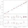 |
Fig. 1 Top panel: best periods obtained for each observation (Col. 6, Table 1) as weighted mean of the folding analysis results performed on single snapshots. The solid line connects the periods extrapolated at the folding epoch times from the radio ephemeris (Col. 8, Table 1). Central panel: residuals between the best periods plotted above and the corresponding periods as extrapolated from the radio ephemeris. Bottom panel: residuals between the periods obtained from the pulse phase analysis (Col. 2, Table 2) and those extrapolated from the radio ephemeris (Col. 8, Table 1). Due to the Y-axis range in the three panels, errors for several points are too small to be visible. |
The precision of the timing parameters can be enhanced by performing a pulse phase analysis on the observations with several snapshots (at least 3). This consists in maintaining a phase pulse coherence over the entire time interval covered by the observation. We have folded the event arrival times of each snapshot with the same epoch time used in the previous analysis and with the observation best period (Col. 6 in Table 1). Phase shifts of the pulse profile are expected because of the indetermination of the period within its error and of the presence of period derivatives. These phase shifts were evaluated by measuring the position of the main peak fitting it with a Lorentzian function plus a constant. The width of the Lorentzian was fixed to the value obtained in the observation with the highest statistics (Obs ID 00058970001). As the main peak has an asymmetric shape, we checked for the presence of systematics in the determination of the peak position due to the choice of the model: fits with a Gaussian function and with a parabola agree within errors with the values obtained with the Lorentzian model, that were therefore used throughout the analysis.
In the absence of frequency irregularities (glitches), the correction to the frequency and its derivative can be obtained by fitting the phase lags by a third degree model:  (4)where Δφ is the measured phase difference at time t, t0 is the epoch time, and Δν0,
  , and
, and  are the correction to the frequency and to its first and second derivative, respectively. The data time span of the Crab observations is not long enough for the second derivative of the frequency to contribute significantly to the phase shift. Therefore the third degree term of the above polynomial is ignored in the fit. Table 2 reports the periods P ∗ (Col. 2) obtained applying Δν0 from Eq. (4) to the periods reported in Table 1, and their associated errors ΔP ∗ (Col. 3) derived as
  , where σΔν0 is the 68% confidence level of Δν0. Differences with respect to the periods extrapolated from the radio ephemeris are reported in Col. 4. The latter are also plotted in the bottom panel in Fig. 1. The pulse phase analysis allows us to obtain an accuracy of the order of tens of picoseconds in the determination of the period, depending on the data time span, down to ~4 ps (ΔP/P ~ 10-9) for the observation with the longest time span (Obs ID 00058970001). The accuracy on the estimate of the first derivative of the period depends both on the length of the data time span and on the number of snapshots; for Obs ID 00058970001 we find a deviation of the period first derivative with respect to the value extrapolated from the radio ephemeris of 0.1%.
4.2. Absolute timing accuracy
Results of the pulse phase analysis performed on the observations with at least 3 snapshots.
The absolute timing of XRT in WT mode was evaluated measuring the phase position of the main pulse peak in the Crab profile obtained folding the XRT data with the radio ephemeris. Observations performed within the same radio ephemeris sample interval were folded together to improve the statistics of the pulse profile. As for the phase analysis, the phase of the main peak was then determined for each profile by fitting it with a Lorentzian function plus a constant. Figure 2 (black diamonds) shows the phase of the main peak vs. time, together with the range of values measured by RXTE (Rots et al. 2004). The positions of the main peak for each XRT observation are not consistent with each other and range between 0.9742 and 0.9885. The pulse profile leads the radio profile and also arrives systematically earlier with respect to the RXTE measure. The average position of the main peak in XRT is at radio phase 0.9817 ± 0.0005, corresponding to ~620 μs earlier than the radio peak and ~270 μs earlier than RXTE.
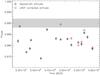 |
Fig. 2 Phase position of the Crab pulsar main peak (black diamonds). The shaded strip marks the phase range where the main peak is measured by RXTE-PCA. Red squares correspond to the phase position measured after correcting the attitude file with UVOT data. Observations with the same radio ephemeris sample interval were folded together and are thus represented by a single point. |
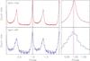 |
Fig. 3 Comparison between the Crab pulse profile obtained with RXTE-PCA (top panels) and that obtained with the Swift-XRT Obs ID 00050100031. The count rates in the Y-axis are in arbitrary units. Vertical lines mark the position of the main peak (red: RXTE-PCA; blue: Swift-XRT). The right panels show a zoom of the main peak interval. |
XRT-PD and BAT Crab observations.
This analysis was also repeated for the observations reduced with the attitude file corrected with UVOT data (see Sect. 3 and first column in Table 1). Figure 2 (red squares) shows the result: the average values of the main peak phase is at 0.9854 ± 0.0002, corresponding to ~490 μs earlier than the radio peak and ~150 μs earlier than RXTE, with a scatter ranging between 0.9801 and 0.9894.
The absolute phase was also verified using the RXTE observation performed simultaneously with Swift-XRT Obs ID 00050100031 (for which only the spacecraft attitude file was available). Given their better time resolution, the RXTE data were folded using 400 phase bins. The XRT data were restricted to the energy range between 2 and 10 keV to better match the RXTE energy selection. The two pulse profiles, obtained folding the data with the radio ephemeris, are shown in Fig. 3. The comparison between the two profiles shows that the position of the main peak observed in XRT is earlier than the RXTE profile with an advance of only 200 ± 38 μs. We have verified that the phase difference is not due to the different spectral content of the two datasets because of the different shape of the effective area in the two instruments: using the observation with the longest time data span (Obs ID 00058970001) we do not observe any significant variation of the main peak phase when selecting in different energy range (2–10 keV, 4–10 keV, 6–10 keV, 8–10 keV). We have also verified that the phase difference is not due to the worse time resolution of the XRT dataset with respect to the RXTE one: we have modified the arrival times of the RXTE events by resampling them with a time resolution of 1.7791 ms and corrected them to the solar system barycenter; the resulting folded profile shows both a broadening (~35%) and a shift (~35 μs in advance) of the main peak. However, this shift is too small to account for the phase difference observed in the XRT profile.
We have checked if the difference in absolute timing observed between RXTE and XRT data in WT mode could also be observed in XRT data collected in PD mode (with 140 μs time resolution) and BAT data collected in event mode (with 100 μs time resolution). We have analyzed all Crab observations with suitable statistics available in the Swift archive. Table 3 reports the details on the observations used for this analysis. We selected PD data in the 2–10 keV range and BAT data in the 15–150 keV range. The barycentered data were analyzed using the same procedure as for the WT data, and the main peak positions obtained with a Lorentzian fit are plotted in Fig. 4. The main peak position obtained by the pulse profiles of the PD mode data are fully consistent with the RXTE result; also for the BAT data we find a good agreement with RXTE. Moreover, for both data sets, the scattering is significantly smaller than that observed in XRT in WT mode.
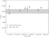 |
Fig. 4 Phase position of the Crab pulsar main peak for XRT-PD (red squares) and BAT (black diamonds) observations. The shaded strip marks the phase range where the main peak is measured by RXTE-PCA. For each instrument, observations with the same radio ephemeris sample interval were folded together and are thus represented by a single point. |
5. Conclusions
We have analyzed the set of Swift-XRT Crab observations in order to qualify the timing performance of the XRT observing in WT mode.
The accuracy in the Crab period determination is mainly limited by the time span covered by the observation with a minimum difference of a few picoseconds with respect to the period extrapolated from radio ephemeris for the longest XRT observation.
We observe a displacement in phase of the Crab pulse profile with respect to the profile observed by RXTE-PCA: the main peak observed in XRT leads the RXTE-PCA one by ~270 μs using the spacecraft attitude files, or ~150 μs when UVOT corrected attitude files are available. This represents a 15% (9% using UVOT attitude files) shift in absolute timing compared to the time resolution of the XRT in WT mode. We have verified that this shift is not due to a spectral effect, nor to the worse time resolution of the XRT dataset with respect to the RXTE one. We observe a significant scatter in the position of the main peak among the XRT observations. Conversely, the peak positions obtained by the analysis of the Crab observations collected by XRT in PD mode and by BAT in event mode are in good agreement with the RXTE measurements. This suggests that the discrepancy observed in XRT WT mode is not due to the Swift spacecraft clock, but most likely to a systematic offset in the time assignment specific to this mode. However, the precision of the pulse period determination in WT mode suggests that the phase offset is stable within each observation even if it is not between observations.
A full description of the time assignment in the Swift FITS files is available at http://swift.gsfc.nasa.gov/docs/swift/analysis/suppl_uguide/time_guide.html
Acknowledgments
The authors wish to thank the anonymous referee for critical review which allowed us to significantly improve the paper. A.P.B. and J.P.O. acknowledge the support of the UK Space Agency. This work has been supported by ASI grant I/011/07/0.
References
- Abbey, T., Carpenter, J., Read, A., et al. 2006, Proceeding of The X-ray Universe 2005, 604, 943 [Google Scholar]
- Barthelmy, S. D., Barbier, L. M., Cummings, J. R., et al. 2005, Space Sci. Rev., 120, 143 [NASA ADS] [CrossRef] [Google Scholar]
- Bradt, H. V., Rothschild, R. E., & Swank, J. H. 1993, A&AS, 97, 355 [NASA ADS] [Google Scholar]
- Burrows, D. N., Hill, J. E., Nousek, J. A., et al. 2005, Space Sci. Rev., 120, 165 [NASA ADS] [CrossRef] [Google Scholar]
- Cusumano, G., Massaro, E., & Mineo, T. 2003, A&A, 402, 647 [NASA ADS] [CrossRef] [EDP Sciences] [Google Scholar]
- Gehrels, N., Chincarini, G., Giommi, P., et al. 2004, ApJ, 611, 1005 [NASA ADS] [CrossRef] [Google Scholar]
- Hill, J. E., Burrows, D. N., Nousek, J. A., et al. 2004, Proc. SPIE, 5165, 217 [NASA ADS] [CrossRef] [Google Scholar]
- Jahoda, K., Markwardt, C. B., Radeva, Y., et al. 2006, ApJS, 163, 401 [NASA ADS] [CrossRef] [Google Scholar]
- Kirsch, M. G. F., Becker, W., Benlloch-Garcia, S., et al. 2004, Proc. SPIE, 5165, 85 [NASA ADS] [CrossRef] [Google Scholar]
- Kuster, M., Kendziorra, E., Benlloch, S., et al. 2002 [arXiv:astro-ph/0203207] [Google Scholar]
- Lorimer, D. R., Kramer, M., Ellis, R., et al. 2004, Handbook of pulsar astronomy, eds. D. R. Lorimer, & M. Kramer, Cambridge observing handbooks for research astronomers, Vol. 4 (Cambridge, UK: Cambridge University Press) [Google Scholar]
- Lyne, A. G., Pritchard, R. S., & Graham-Smith, F. 1993, MNRAS, 265, 1003 [NASA ADS] [CrossRef] [Google Scholar]
- Molkov, S., Jourdain, E., & Roques, J. P. 2010, ApJ, 708, 403 [NASA ADS] [CrossRef] [Google Scholar]
- Roming, P. W. A., Kennedy, T. E., Mason, K. O., et al. 2005, Space Sci. Rev., 120, 95 [NASA ADS] [CrossRef] [Google Scholar]
- Rots, A. H., Jahoda, K., & Lyne, A. G. 2004, ApJ, 605, L129 [NASA ADS] [CrossRef] [Google Scholar]
- Terada, Y., Enoto, T., Miyawaki, R., et al. 2008, PASJ, 60, 25 [NASA ADS] [Google Scholar]
All Tables
Results of the pulse phase analysis performed on the observations with at least 3 snapshots.
All Figures
|
Fig. 1 Top panel: best periods obtained for each observation (Col. 6, Table 1) as weighted mean of the folding analysis results performed on single snapshots. The solid line connects the periods extrapolated at the folding epoch times from the radio ephemeris (Col. 8, Table 1). Central panel: residuals between the best periods plotted above and the corresponding periods as extrapolated from the radio ephemeris. Bottom panel: residuals between the periods obtained from the pulse phase analysis (Col. 2, Table 2) and those extrapolated from the radio ephemeris (Col. 8, Table 1). Due to the Y-axis range in the three panels, errors for several points are too small to be visible. |
| In the text | |
|
Fig. 2 Phase position of the Crab pulsar main peak (black diamonds). The shaded strip marks the phase range where the main peak is measured by RXTE-PCA. Red squares correspond to the phase position measured after correcting the attitude file with UVOT data. Observations with the same radio ephemeris sample interval were folded together and are thus represented by a single point. |
| In the text | |
|
Fig. 3 Comparison between the Crab pulse profile obtained with RXTE-PCA (top panels) and that obtained with the Swift-XRT Obs ID 00050100031. The count rates in the Y-axis are in arbitrary units. Vertical lines mark the position of the main peak (red: RXTE-PCA; blue: Swift-XRT). The right panels show a zoom of the main peak interval. |
| In the text | |
|
Fig. 4 Phase position of the Crab pulsar main peak for XRT-PD (red squares) and BAT (black diamonds) observations. The shaded strip marks the phase range where the main peak is measured by RXTE-PCA. For each instrument, observations with the same radio ephemeris sample interval were folded together and are thus represented by a single point. |
| In the text | |
Current usage metrics show cumulative count of Article Views (full-text article views including HTML views, PDF and ePub downloads, according to the available data) and Abstracts Views on Vision4Press platform.
Data correspond to usage on the plateform after 2015. The current usage metrics is available 48-96 hours after online publication and is updated daily on week days.
Initial download of the metrics may take a while.