| Issue |
A&A
Volume 692, December 2024
|
|
|---|---|---|
| Article Number | A234 | |
| Number of page(s) | 6 | |
| Section | Astronomical instrumentation | |
| DOI | https://doi.org/10.1051/0004-6361/202450557 | |
| Published online | 16 December 2024 | |
Tracking the long-term timing accuracy of the X-Ray Telescope on board the Neil Gehrels Swift Observatory
1
INAF – Istituto di Astrofisica Spaziale e Fisica Cosmica di Palermo,
Via U. La Malfa 153,
90146
Palermo,
Italy
2
INAF – Osservatorio Astronomico di Roma,
Via Frascati 33,
00078
Monte Porzio Catone,
Italy
3
Space Science Data Center (SSDC), Agenzia Spaziale Italiana,
Via del Politecnico snc,
00133
Rome,
Italy
4
Department of Physics and Astronomy, University of Leicester,
University Road,
Leicester
LE1 7RH,
UK
5
Department of Astronomy and Astrophysics, The Pennsylvania State University,
525 Davey Laboratory, University Park,
Pennsylvania
16802,
USA
6
INAF – Osservatorio Astronomico di Brera,
Via Bianchi 46,
23807
Merate,
Italy
★ Corresponding author; This email address is being protected from spambots. You need JavaScript enabled to view it.
Received:
30
April
2024
Accepted:
12
November
2024
Abstract
Context. The Neil Gehrels Swift Observatory has been operational since November 2004. Its X-ray Telescope (XRT), operating in the 0.3–10.0 keV range, is designed to provide detailed position, timing, and spectroscopic information.
Aims. The calibration procedure for assessing the absolute timing accuracy of XRT was described in a previous paper. Here we update the past analysis using the complete data set of the Crab pulsar observations up to October 2022 and using a new version of the data-processing software package that includes corrections to several issues that could have affected the previous results.
Methods. We evaluate the accuracy of the Crab pulse period determination using the folding technique and the pulse-phase analysis and compare our results with the values derived from radio observations. We also check the absolute time reconstruction, measuring the phase position of the main peak in the Crab profile and comparing it with the value reported in the literature, which is based on Rossi X-Ray Timing Explorer (RXTE) observations.
Results. We find that the accuracy in period determination for the Crab pulsar is of the order of a few picoseconds for the observations with the largest data time span. The absolute time reconstruction, measured using the position of the main pulse peak, shows that the main peak precedes the phase of the position reported in the literature for RXTE by ~263 µs on average. This corresponds to 0.982 in phase, with an observed dispersion of ±0.02 in phase values. We also find that observations very close in time (down to ~1 day separation) show a significant variation in absolute phase.
Key words: instrumentation: detectors / methods: data analysis / telescopes / pulsars: individual: PSR J0534+2200
© The Authors 2024
 Open Access article, published by EDP Sciences, under the terms of the Creative Commons Attribution License (https://creativecommons.org/licenses/by/4.0), which permits unrestricted use, distribution, and reproduction in any medium, provided the original work is properly cited.
This article is published in open access under the Subscribe to Open model. This email address is being protected from spambots. You need JavaScript enabled to view it. to support open access publication.
1 Introduction
The Neil Gehrels Swift Observatory (Gehrels et al. 2004) is a multi-wavelength space facility that operates in the optical- UV, X-ray, and soft gamma-ray ranges. This is accomplished through its three telescopes: the UltraViolet and Optical Telescope (UVOT; Roming et al. 2005), which covers a wavelength range of 170–650 nm; the X-Ray Telescope (XRT; Burrows et al. 2005) operating in the 0.3–10 keV energy range; and the Burst Alert Telescope (BAT; Barthelmy et al. 2005) observing in the 15–350 keV band. The observatory’s main goal is the prompt detection of gamma-ray bursts (GRBs) and rapid follow-up of their X-ray and UV afterglows, with over 1500 GRBs observed to date. In addition to its primary mission, a significant portion of observing time is dedicated to other X-ray sources (both transient and persistent), either as targets of opportunity or through monitoring programs.
Calibration and continuous monitoring of performance are fundamental factors in the optimal exploitation of any instrument. In this paper, we focus on the verification of the timing accuracy of XRT in its fast-timing operating mode, windowed timing (WT). This is achieved through a campaign of regularly planned observations of the Crab pulsar (PSR J0534+2200). The Crab pulsar (with a period of ∼33 ms) has served the purpose of in-flight calibration for several telescopes (e.g. Kuster et al. 2002; Rots et al. 2004; Kirsch et al. 2004; Terada et al. 2008; Molkov et al. 2010; Martin-Carrillo et al. 2012; Basu et al. 2021; Bachetti et al. 2021; Tuo et al. 2022; Xiao et al. 2024) since its timing properties are continuously monitored in the radio and its ephemeris is regularly updated on a monthly basis and is made available by the Jodrell Bank Observatory1. Its pulse profile is characterised over the entire electromagnetic spectrum by a double peak with a phase separation of ∼0.4, although the overall shape depends on the energy band. RXTE found that the profile in the 2–16 keV energy band precedes the radio profile by 344±40 µs (0.0102 ± 0.0012 in phase (Rots et al. 2004). This result is adopted as a reference for the calibration of the absolute timing of any telescope operating in the X-ray band.
The XRT, equipped with a single e2v CCD-22 imaging detector at its focal plane, was designed to support four different data read-out modes (see Hill et al. 2004 for an exhaustive description) in order to have a wide and dynamic observable flux range and follow rapid variability of transient phenomena. Here, we focus on the WT mode, which is the mode with the highest time resolution (1.7791 ms) after the Photo-Diode mode, which was characterised by a timing resolution of 0.14 ms, but was disabled following a micrometeorite hit on May 27, 2005.
The timing performance verification of XRT has been the subject of a previous paper (Cusumano et al. 2012), where we analysed the Crab pulsar observations up to January 2012, showing that the accuracy in the period determination is of the order of some tens of picoseconds, and the absolute time reconstruction anticipates the phase of the position reported in the literature for RXTE by ~270 µs.
In the present work, we update those results by including all the Crab observations up to October 2022. This analysis is strongly motivated by relatively recent changes to multi-mission tasks (see Sect. 3) that play a crucial role in this study. For this reason, we also reanalysed the previous observations in order to produce a uniform dataset and to obtain a firm assessment of the timing accuracy of the XRT.
The paper is organised as follows: Section 2 briefly describes how photon events in WT mode are time-tagged; Sect. 3 summarises the XRT observations of the Crab pulsar, and the data reduction procedure; Sect. 4 describes the timing analysis and its results; and in Sect. 5 we conclude with a brief summary of the results.
2 Reconstruction of photon arrival times in WT mode
In WT mode, the CCD rows are continuously clocked and are binned by a factor of 10 along the Y direction before the readout. The photon arrival times are calculated during the ground processing by a specific software module, named XRTTIMETAG, which is included in the XRT Data Analysis Software (XRT- DAS2) package. The reconstruction of the time tag of the events makes use of information present in the telemetry and the celestial coordinates of the target. A detailed description of the WT time-tag algorithm can be found in our previous paper (Cusumano et al. 2012). Here we simply note that this algorithm requires knowledge of the location of the X-ray source on the detector, and for this reason the accuracy of the spacecraft attitude reconstruction is a key factor in the calculation of the photon’s arrival time. We note that, in this work, the attitude file derived using the UVOT data (UAT), which is in principle the most accurate spacecraft attitude file available in the Neil Gehrels Swift Observatory archive, was not considered. This is due to the fact that the UAT files intrinsically include corrections for the UVOT time-dependent boresight and this correction is not suitable for the XRT processing. For this reason, since January 2014, the XRT pipeline processing does not allow its use. The jump-corrected attitude file (PAT) was instead used in this paper.
3 Observation and data reduction
We analysed 76 Crab pulsar observations (from 2005 to 2022) performed with the XRT in WT mode for which valid radio ephemeris data are available and where the pulsar is always less than 5 arcmin from the on-axis direction. This choice excludes the observations where the pulsar is at the edge of or outside the WT image strip. The Level 1 data were retrieved from the HEASARC public data archive3 and calibrated, filtered, and screened with the XRTDAS package included in the HEASoft 6.32.1 software release using default processing parameters.
The source events with grade 0–2 were extracted from each observation using a rectangular region of 40 pixel in width centred on the pixel with the highest number of counts. This region includes ~ 94% of the point spread function of the Crab pulsar, which is located near the centre of the Nebula. The arrival times of each event were translated to the Solar System Barycentre (SSB) using the Crab coordinates, right ascension (RA) = 05h 34m 31.972s, declination (Dec) = 22°00′ 52".07 (Lyne et al. 1993), the JPL DE200 Solar System ephemeris, and the barycentrization code BARYCORR, which also takes into account the time drift occurring during the observation through the mission clockfile (swclockcor20041120v160.fits, updated to 2024 May 06) and the spacecraft orbit through the ObsID specific attorb file.
An important factor in the barycentre-correction procedure is the accuracy of the spacecraft orbit. During the pipeline processing, the multi-mission task PREFILTER of the HEASoft package is run for the determination of attitude and orbit-related quantities. An imprecision in the calculation of the spacecraft location, not taking into account the Swift UTC clock correction factor, was pointed out in 2017 and was resolved in the 6.20 version of the package. As the satellite orbit information – included in a dedicated file – is given as input to BARYCORR, the accuracy of the barycentre corrections were affected by this issue before the code fix. In addition, extensive changes have been made to the BARYCORR code (included in HEASoft v6.32.1), although no significant impact on the output corrections is expected. As mentioned in Sect. 1, the latest version of the software has been used for the processing of the whole dataset, allowing more accurate results. Table A.1 reports the details of the observations used for the analysis. Several observations are split into multiple snapshots, because of the low-inclination equatorial orbit of the satellite and the optimisation strategy adopted for the pointing plan. Each snapshot lasts from a few hundreds of seconds to -1 ks, and snapshots are separated by one or more orbits (-96 minutes).
4 Timing analysis and results
In order to derive the Crab pulse period, we apply a folding technique to the data (e.g. Lorimer et al. 2004). However, as opposed to Cusumano et al. (2012), where this method was applied to each single snapshot and the resulting best periods obtained in the same ObsID were averaged, in this work we apply the folding method to the entire ObsID, with the larger time baseline allowing for a narrower χ2 peak, and consequently a lower uncertainty on the period estimation.
4.1 Accuracy of the Crab period estimation
We used the following procedure to derive the best period for each ObsID listed in Table A.1:
We applied a folding analysis to the barycentred arrival times in each observation. We fixed the folding epoch time to the observation central time (Tepoch, column 5 in Table A.1), and using the Crab radio ephemeris (in CGRO format) provided by the Jodrell Bank Observatory, we searched in a period range centred on the expected period4 (column 6 in Table A.1). The period search was performed with a step resolution of ∆P = P2/(N∆T), where N = 300 is the number of phase bins used to sample the pulse profile and ∆T is the observation elapsed time (column 2 in Table A.1).
For each observation, we derived the best period (Pfold, column 7 in Table A.1) by fitting the resulting χ2 peak with a Lorentzian profile. The error on the best period (the digit in parentheses) was evaluated as the period interval corresponding to a unit decrement with respect to the maximum in the χ2 curve (Cusumano et al. 2003), that is,
 .
.
In the top panel of Fig. 1 we compare the best periods obtained in this work (diamond points) to those derived from the radio ephemeris (solid line). The central panel shows the residuals with respect to the values extrapolated from the radio ephemeris (see also column 8 in Table A.1). The folding analysis on these observations allows us to obtain an accuracy of the order of a few tens of picoseconds to some tens of nanoseconds on the determination of the period, depending on the data time span and on the number of snapshots of each observation.
Comparing our results with those reported for the same ObsIDs in Table 1 of Cusumano et al. (2012), we observe that the discrepancy between the period evaluated in this work with the folding method and the radio period is in most cases significantly smaller than previously reported. This improvement is evident in the ObsIDs with more than one snapshot, and is due to the change in methodology.
The precision of the period for the ObsIDs with at least three snapshots may be improved by performing a pulse-phase analysis. This consists in folding the data of each single snapshot within an ObsID using the period obtained by folding the entire ObsID (Pfold in column 7 of Table A.1) while keeping Tepoch to the ObsID central time (column 5 in Table A.1). If there is a significant mismatch between the true period at Tepoch (column 6 in Table A.1) and Pfold, we see a shift in the snapshot pulse profile. The main peak in each snapshot profile can then be fitted to evaluate its position in phase (we used a Lorentz function plus a constant) and reconstruct how the peak shifts in time. These phase lags can be used to obtain a correction to the frequency and its derivatives by fitting, for each ObsID, the phase shift versus time with a third-degree polynomial function:
 (1)
(1)
where Δϕ is the measured phase difference at time t (the centre of the snapshot), Tepoch is the epoch time, and Δν0,  , and
, and  are the correction to the frequency and its first and second derivatives, respectively. As the data time span of the Crab observations is not long enough to be sensitive to the second spin-frequency derivative, the third-degree term of the above polynomial is ignored in the fit.
Our sample includes 37 observations where this correction can be applied, as they all have at least three snapshots. Table 1 reports the periods P* (column 2) obtained applying Δν0 from Eq. (1) on the best periods reported in Table A.1 (column 7), with errors evaluated as  , where
  is the 68% confidence level of Δν0. Column 3 reports the differences with respect to the periods extrapolated from the radio ephemeris (see also the bottom panel in Fig. 1); column 4 reports the absolute value of the ratio between the values in column 3 and the corresponding values in column 8 of Table A.1. A value of lower than 1 indicates a significant improvement in the period evaluation, which is obtained for the majority of observations. For some observations, we do not obtain an improvement as the discrepancy with the radio period was already very small (down to 1 ps for ObsID 00050100039) and the linear coefficient of the above expression is consistent with zero. On the other hand, we observe that, as expected, this method is more efficient if applied to long observations with a large number of snapshots.
The pulse-phase analysis allows us to obtain, in the best cases, an accuracy of down to a few picoseconds in the determination of the period. The RMS of the difference between the radio periods and our results (evaluated only for the 37 observations with three or more snapshots) goes from 2.20 ns (with the folding method) to 0.46 ns (using the phase-shift correction). We also evaluated the accuracy of the estimate of the first derivative of the period for the longest observation (ObsID 00058970001), finding a deviation with respect to the value extrapolated from the radio ephemeris of 0.1%.
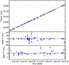 |
Fig. 1 Period estimation and comparison with the radio measurements. Top panel: best periods obtained with the folding analysis for each observation (column 7, Table A.1). The solid line connects the periods extrapolated at the folding epoch times from the radio ephemeris (column 6, Table A.1). Central panel: residuals between the best periods plotted above and the corresponding periods as extrapolated from the radio ephemeris (column 8, Table A.1). The three points where this difference is higher than 40 ns are excluded from the plot for improved clarity. Bottom panel: residuals between the periods obtained from the pulse-phase analysis and those extrapolated from the radio ephemeris (column 3, Table 1). Due to the Y -axis range in the three panels, errors for several points are too small to be visible. |
4.2 Absolute timing accuracy
In order to evaluate the absolute timing of XRT in WT mode, we studied the phase position of the main pulse peak in the Crab profiles obtained by folding each XRT observation with the corresponding radio ephemeris. The relevant time of zero radio phase (tgeo) has been used as tepoch after reporting it to the SSB using the JPL DE200 Solar System ephemeris and the list of leap seconds updated to December 31, 2016. We compared the resulting X-ray profile with the radio profile to evaluate the phase shift. While in Cusumano et al. (2012) observations performed within the same radio ephemeris interval were folded together to improve the statistics of the pulse profile, here we produce a profile for each ObsID. The main peak position in each profile was determined by fitting it in a phase interval of ±0.07 around the top with a Lorentzian function plus a constant. The errors associated with the peak position are at the 68% confidence level. Figure 2 shows the phase of the main peak versus time, together with the range of values measured by RXTE (Rots et al. 2004). The dispersion of the phase values is significantly larger than the associated errors, ranging between 0.96 and 1.00. The average position of the main peak in XRT is at phase 0.982 (with standard deviation 0.008), which corresponds to ∼607 µs earlier than the radio peak and ∼263 µs earlier than RXTE. The plot also shows that observations that are very close in time (down to ∼1 day separation) may have a large span in absolute phase.
Results of the pulse-phase analysis performed on the observations with at least three snapshots.
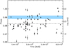 |
Fig. 2 Phase position of the Crab pulsar main peak. The right axis represents the phase delay in ms derived using a radio period of 33.7 ms (averaged over the data set). The dashed line represents the position of the main peak averaged over the entire dataset. The shaded strip centred at 0.9898 marks the phase range where the main peak is measured by RXTE (Rots et al. 2004), with its width dominated by a systematic uncertainty of 0.0012. |
5 Conclusions
This paper updates the results reported in Cusumano et al. (2012) on the timing accuracy of the WT mode of the XRT instrument on board the Neil Gehrels Swift Observatory by adding all the observations performed from November 2012 to October 2022 to the previous dataset, for a total of 76 Crab observations. We reprocessed and reanalysed the entire dataset with the latest reduction package and with a different strategy with respect to Cusumano et al. (2012). This allowed us to improve the accuracy on the determination of the period, with the folding analysis results reaching an order of a few tens of picoseconds to some tens of nanoseconds, depending on the data time span and on the number of snapshots within each observation. When possible (i.e. for observations with three or more snapshots), we used the pulse-phase analysis, obtaining a general improvement of the accuracy, which in some cases was reduced to a few picoseconds, with an improvement in the RMS of the differences between the radio periods and the values derived in this paper of a factor of ∼5.
We evaluated the absolute timing, studying the phase of the main peak in the Crab pulse profile. We find the dispersion of the phase values to be significantly larger than the associated errors, and to range between 0.96 and 1.00 among the different observations. This dispersion was less pronounced in Cusumano et al. (2012), where ObsIDs within the same radio ephemeris interval were folded together. Here, folding each ObsID separately, we find that observations very close in time (down to ∼1 day separation) show significant variation in absolute phase. The average position of the main peak in XRT is at phase 0.982 with a standard deviation of 0.008, which corresponds to ∼607 µs earlier than the radio peak and ∼263 µs earlier than the peak phase determined with RXTE.
Our overall results regarding the absolute phase are consistent with the conclusions of Cusumano et al. (2012), where the absolute phase was also evaluated for the XRT Photo-Diode mode data and for the BAT data, with the authors finding them to be in a good agreement with the RXTE measurements. These authors proposed that the phase discrepancy observed in XRT WT mode was therefore most likely attributable to an offset in the time assignment specific to this mode, which varies among different observations.
Acknowledgements
The authors wish to thank the anonymous referee for their useful comments that helped us improving the paper. This work has been supported by ASI grant I/011/07/5. This research has made use of the XRT Data Analysis Software (XRTDAS) developed under the responsibility of the ASI Space Science Data Center (SSDC), Italy.
Appendix A Additional table
Observation log and period search results (folding method).
References
- Bachetti, M., Markwardt, C. B., Grefenstette, B. W., et al. 2021, ApJ, 908, 184 [CrossRef] [Google Scholar]
- Barthelmy, S. D., Barbier, L. M., Cummings, J. R., et al. 2005, Space Sci. Rev., 120, 143 [Google Scholar]
- Basu, A., Bhattacharya, D., & Joshi, B. C. 2021, J. Astrophys. Astron., 42, 61 [NASA ADS] [CrossRef] [Google Scholar]
- Burrows, D. N., Hill, J. E., Nousek, J. A., et al. 2005, Space Sci. Rev., 120, 165 [Google Scholar]
- Cusumano, G., Massaro, E., & Mineo, T. 2003, A&A, 402, 647 [NASA ADS] [CrossRef] [EDP Sciences] [Google Scholar]
- Cusumano, G., La Parola, V., Capalbi, M., et al. 2012, A&A, 548, A28 [NASA ADS] [CrossRef] [EDP Sciences] [Google Scholar]
- Gehrels, N., Chincarini, G., Giommi, P., et al. 2004, ApJ, 611, 1005 [Google Scholar]
- Hill, J. E., Burrows, D. N., Nousek, J. A., et al. 2004, Proc. SPIE, 5165, 217 [NASA ADS] [CrossRef] [Google Scholar]
- Kirsch, M. G. F., Becker, W., Benlloch-Garcia, S., et al. 2004, Proc. SPIE, 5165, 85 [NASA ADS] [CrossRef] [Google Scholar]
- Kuster, M., Kendziorra, E., Benlloch, S., et al. 2002 [arXiv:astro-ph/0203207] [Google Scholar]
- Lorimer, D. R., Kramer, M., Ellis, R., et al. 2004, Handbook of Pulsar Astronomy, Cambridge observing handbooks for research astronomers, eds. D.R. Lorimer, & M. Kramer (Cambridge, UK: Cambridge University Press), 4 [Google Scholar]
- Lyne, A. G., Pritchard, R. S., & Graham-Smith, F. 1993, MNRAS, 265, 1003 [Google Scholar]
- Martin-Carrillo, A., Kirsch, M. G. F., Caballero, I., et al. 2012, A&A, 545, A126 [NASA ADS] [CrossRef] [EDP Sciences] [Google Scholar]
- Molkov, S., Jourdain, E., & Roques, J. P. 2010, ApJ, 708, 403 [NASA ADS] [CrossRef] [Google Scholar]
- Roming, P. W. A., Kennedy, T. E., Mason, K. O., et al. 2005, Space Sci. Rev., 120, 95 [Google Scholar]
- Rots, A. H., Jahoda, K., & Lyne, A. G. 2004, ApJ, 605, L129 [NASA ADS] [CrossRef] [Google Scholar]
- Terada, Y., Enoto, T., Miyawaki, R., et al. 2008, PASJ, 60, 25 [NASA ADS] [Google Scholar]
- Tuo, Y., Li, X., Ge, M., et al. 2022, ApJS, 259, 14 [NASA ADS] [CrossRef] [Google Scholar]
- Xiao, S., Liu, Y.-Q., Gong, K., et al. 2024, ApJS, 270, 3 [NASA ADS] [CrossRef] [Google Scholar]
The expected period is extrapolated according to the following expression:  where
where  are the Crab radio ephemeris at time Trad.
All Tables
Results of the pulse-phase analysis performed on the observations with at least three snapshots.
All Figures
|
Fig. 1 Period estimation and comparison with the radio measurements. Top panel: best periods obtained with the folding analysis for each observation (column 7, Table A.1). The solid line connects the periods extrapolated at the folding epoch times from the radio ephemeris (column 6, Table A.1). Central panel: residuals between the best periods plotted above and the corresponding periods as extrapolated from the radio ephemeris (column 8, Table A.1). The three points where this difference is higher than 40 ns are excluded from the plot for improved clarity. Bottom panel: residuals between the periods obtained from the pulse-phase analysis and those extrapolated from the radio ephemeris (column 3, Table 1). Due to the Y -axis range in the three panels, errors for several points are too small to be visible. |
| In the text | |
|
Fig. 2 Phase position of the Crab pulsar main peak. The right axis represents the phase delay in ms derived using a radio period of 33.7 ms (averaged over the data set). The dashed line represents the position of the main peak averaged over the entire dataset. The shaded strip centred at 0.9898 marks the phase range where the main peak is measured by RXTE (Rots et al. 2004), with its width dominated by a systematic uncertainty of 0.0012. |
| In the text | |
Current usage metrics show cumulative count of Article Views (full-text article views including HTML views, PDF and ePub downloads, according to the available data) and Abstracts Views on Vision4Press platform.
Data correspond to usage on the plateform after 2015. The current usage metrics is available 48-96 hours after online publication and is updated daily on week days.
Initial download of the metrics may take a while.