| Issue |
A&A
Volume 548, December 2012
|
|
|---|---|---|
| Article Number | A80 | |
| Number of page(s) | 8 | |
| Section | The Sun | |
| DOI | https://doi.org/10.1051/0004-6361/201219640 | |
| Published online | 26 November 2012 | |
A cross-correlation method for measuring line formation heights in the solar photosphere
Laboratoire Lagrange, UMR 7293, Université de Nice Sophia Antipolis, CNRS,
Observatoire de la Côte d’Azur,
Campus Valrose,
06108
Nice,
France
e-mail: This email address is being protected from spambots. You need JavaScript enabled to view it.
; This email address is being protected from spambots. You need JavaScript enabled to view it.
; This email address is being protected from spambots. You need JavaScript enabled to view it.
Received:
21
May
2012
Accepted:
14
September
2012
Abstract
Context. Detailed 3D-simulations of magneto-convection in the solar photosphere are now available. They intend to capture the main physical mechanisms at play in this boundary layer, where complex physical phenomena, such as convective overshooting and small scale magnetic dynamo take place. But numerical limitations in spatial resolution and in box-size are likely to affect the description of some relevant physical scales, so simulations need to be compared to independent observations allowing us to explore the full height range of the photosphere.
Aims. Here we focus on a model-independent method for measuring line formation depths. We construct images of the photosphere at constant continuum opacity levels from the low to the upper photosphere and we show how they can be used to measure systematic displacements of granular structures with height. The method is applied to determine the formation height of the 630 nm Fe i line pair. We compare our measurements to the results of 3D simulations.
Methods. We analyze high resolution spectroscopic scans obtained in the 630 nm Fe i line pair at varying heliocentric angles along the north-south polar axis of the Sun, with SOT onboard Hinode. We implement a new strategy for correcting the images observed at different line cords from spurious Doppler effects. The cross-correlations between continuum images and line core images show a clear anti-correlation peak due to the contrast inversion of the granulation in the upper photosphere, as predicted by magnetohydrodynamic (MHD) simulations.
Results. The anti-correlation peak is shifted by the perspective effect and by horizontal velocity effects. Both effects may be distinguished because they have different center-to-limb variations. The measurement of the perspective shift allows us to determine the line core formation heights and their center-to-limb variations. The results are in good agreement with 3D- MHD simulations for images close to disk center, but close to the solar limb we measure larger formation heights than what is predicted by the simulations, which seem to fail in modeling properly the upper layers of the photosphere. As the granulation contrast inversion is observed at line centers, we can safely conclude that the height of the contrast inversion layer is smaller than 200 km.
Key words: line: formation / techniques: imaging spectroscopy / Sun: photosphere
© ESO, 2012
1. Introduction
Solar surface dynamics is driven by turbulent convection, magnetic fields and the escape of radiation. The interplay of all these physical phenomena leads to the complex 3D structure observable in the photosphere. Numerical simulations of magneto-convection taking into account the escape of radiation are now available (Stein & Nordlund 1998, 2006). However the turbulent nature of the flows implies the interaction between many scales either in the velocity field or in the magnetic field or between both. Numerical simulations are probably far from handling all the relevant scales, direct observations are thus needed to test the numerical models and to guide their further development. A large number of papers have been devoted to this kind of comparisons. They allowed, for example to recover the C-shape of the average photospheric line profiles (Asplund et al. 2000), and the intensity fluctuations spatial spectrum observed in the low photosphere (Wedemeyer-Böhm & Rouppe van der Voort 2009). However, it seems that up to now few studies have been carried out to explore the depth variations of the photosphere over its full height range. The BaII line at 455.4 nm was used by Kostik et al. (2009) to probe the granulation up to the low chromosphere, however this strong resonance line is affected by non-local thermodynamic equilibrium (LTE). In order to directly relate brightness fluctuations to temperature fluctuations, without referring to a model of line formation, one has to use lines formed under local thermodynamic equilibrium. Here we focus on the upper photosphere where the cores of the 630 nm Fe i line pair are formed. The 630 nm Fe i line pair is a good candidate because deviations from LTE affect only weakly the emergent intensity profiles in these lines. The largest non-LTE effets appear at line center where the relative difference between profiles computed under LTE or non-LTE conditions remain smaller than 10%, as shown by Shchukina & Trujillo Bueno (2001) (Figs. 11 and 14).
Here we use high resolution spectroscopic scans of the granulation obtained in these lines with SOT onboard Hinode, on December 19, 2007. At this date the angle of the solar rotation axis B0 = −1,4°, so the equator is almost perpendicular to the plane of the sky. The 1024 pixel-spectrograph slit parallel to the north-south polar axis of the Sun was successively located at 20 latitudes allowing us to scan continously the full center-to-limb variations of the solar disk image. At each location a 380-step west-east scan was performed, with a step size of 0.16 arcsec. The pixel size along the slit is 0.16 arcsec, this limits the spatial resolution of the images to 0.32 arcsec (the diffraction limit of the 50 cm miror of the telescope is 0.24 arcsec in the visible domain at 630 nm, the images are thus slightly under-sampled by SOT/SP cameras). As each 380 × 1024 image covers a large part (164 arcsec) of the solar diameter, we divide it into eight 380 × 128 images (60.8′′ × 20′′), where we assume that the value of the heliocentric angle remains approximately constant (we consider its value at the central pixel). The spectral resolution of the SOT spectrograph is 2.15 nm/px in our spectral domain between 630.08 and 630.32 nm. The observational data we analyze in this paper then consist of (380 × 128) images at 160 successive heliocentric angles along the solar diameter and at 112 wavelengths scanning both lines.
In the second section we present the method that we have implemented in order to extract from the spectroscopic scans, images of the photosphere at 25 continuum optical depth levels, from the base of the photosphere to the upper layers where the line cores are formed, for the full set of 160 heliocentric angles. The third section is devoted to the analysis of the cross-correlations of continuum images with images obtained at various levels in the lines. At disk center, the cross-correlations with images observed in the line cores show a clear negative “anti-correlation” peak, at the origin, whereas we observe a positive correlation peak with levels located closer to the continuum. Out of the solar disk center, we observe both a correlation peak at the origin and a negative anti-correlation peak shifted towards the north for images obtained in the northern hemisphere, and towards the south in the southern hemisphere. The negative peak is due to the contrast inversion of the granulation which appears in the upper photosphere, as predicted by numerical models (Cheung et al. 2007). We show how this can be used to determine the line formation heights.
2. Photospheric images at constant continuum optical depths
The images that we observe in the continuum are “formed” over a small layer of the
photosphere, typically localized around the height where the optical thickness of the
photosphere at the wavelength of the observation is equal to one (this is the so-called
Eddington-Barbier approximation). As the opacity varies along the solar surface because of
the photospheric inhomogeneities of density and temperature, the formation height of an
image is not constant over the solar surface. Furthermore, because of the physics of
radiation transport, the images are “optical averages” over a typical photon mean-free path
of the actual temperature and density structures at the optical depth unity level. When
observations are performed in a spectral line, the opacity varies steeply with the
wavelength. It is given by  (1)where
kc is the continuum opacity, kl is
the frequency-averaged line opacity, λ0 is the line center
wavelength in the observer’s frame, and φ is the normalized absorption
profile, which goes to zero on a Doppler width scale ΔλD,
typically. The Doppler broadening is due both to thermal broadening and to unresolved
velocities. It is important to notice that φ is a function of the “reduced”
wavelength variable
δλ = (λ − λ0)/ΔλD,
depending both on the line center wavelength and on the Doppler width. These two quantities
vary over the solar surface because of granular structures. So the opacity at a given
wavelength λ, may vary significantly at small scale and the image observed
at a given wavelength in the line profile mixes signals originating from various structures
located at very different depths in the photosphere. So, getting meaningful informations on
the 3D structure of the photosphere from 2D spectroscopic observations in a spectral line is
not a trivial task!
(1)where
kc is the continuum opacity, kl is
the frequency-averaged line opacity, λ0 is the line center
wavelength in the observer’s frame, and φ is the normalized absorption
profile, which goes to zero on a Doppler width scale ΔλD,
typically. The Doppler broadening is due both to thermal broadening and to unresolved
velocities. It is important to notice that φ is a function of the “reduced”
wavelength variable
δλ = (λ − λ0)/ΔλD,
depending both on the line center wavelength and on the Doppler width. These two quantities
vary over the solar surface because of granular structures. So the opacity at a given
wavelength λ, may vary significantly at small scale and the image observed
at a given wavelength in the line profile mixes signals originating from various structures
located at very different depths in the photosphere. So, getting meaningful informations on
the 3D structure of the photosphere from 2D spectroscopic observations in a spectral line is
not a trivial task!
2.1. Corrections of Doppler effects
In this work we have implemented a method which allows us to recover images formed in layers located at constant continuum optical depths. Introducing the line strength r = kl/kc, we can write the opacity as k(λ) = kc(1 + rφ(δλ)). In order to recover the photospheric structures at given continuum opacity levels from the spectroscopic scans, we need to build images at constant values of (1 + rφ(δλ)) over the observed solar surface.
Line-of-sight velocities due to granular motions and to 5 mn-oscillations have two effects on the line absorption profile. First, the line center wavelength λ0 is shifted, this yields to a shift of the line intensity minimum which is centered at varying values of λ from pixel-to-pixel in the image. The second effect is due to unresolved line-of-sight velocities and/or to their depth-gradients, which affect the observed line width and the line asymmetry. These two physical effects lead to variations of the opacity k(λ), at a given λ value, over the solar surface, both because of the variation of λ0 and of the line Doppler width. Furthermore, variations of temperature and density due to the presence of structures also modify the local Doppler width and the line strength r. So, in order to extract from 2D spectroscopic scans images of the solar photosphere at constant continuum opacity levels kc(1 + rφ(δλ)), we have to pick at each pixel the line intensity at a given value of rφ(δλ).
This is achieved in the following way. At each pixel along the spectrograph slit, we
first define the line cord Δλc, as the line cord where the
intensity is close to the continuum intensity, namely 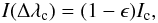 (2)where
Ic denotes the continuum intensity. We cannot measure the
line cord width at the continuum level because, rigorously speaking, it not well defined,
as φ(δλ) tends to zero when δλ tends to
infinity. On a more pragmatic point of view, the continuum level is not reached in between
the two lines because the two line wings overlap. So it is safer to define
Δλc from a well defined intensity level, close enough to the
continuum. The precise value of ϵ is not critical, as long as it is small
and identical for all the pixels. At this line cord the line depression is small and thus
proportional to the line opacity (this corresponds to the linear regime of the curve of
growth), so we can assume that
rφ(Δλc/ΔλD) ≃ ϵ,
is constant for all the pixels in the image. Then, we consider 25 evenly distributed cords
defined by
Δλi/Δλc = i/24,
where the index i varies from 0 at line center to 24, and we build 25
images by extracting the line intensity at these reduced line cords for all the spectra in
our scan. Let us stress that the line cords
Δλi are not constant over the image, as
Δλc varies from pixel to pixel, but the reduced cord grid,
which is the relevant quantity as far as the opacity is concerned, is uniform over the
image.
(2)where
Ic denotes the continuum intensity. We cannot measure the
line cord width at the continuum level because, rigorously speaking, it not well defined,
as φ(δλ) tends to zero when δλ tends to
infinity. On a more pragmatic point of view, the continuum level is not reached in between
the two lines because the two line wings overlap. So it is safer to define
Δλc from a well defined intensity level, close enough to the
continuum. The precise value of ϵ is not critical, as long as it is small
and identical for all the pixels. At this line cord the line depression is small and thus
proportional to the line opacity (this corresponds to the linear regime of the curve of
growth), so we can assume that
rφ(Δλc/ΔλD) ≃ ϵ,
is constant for all the pixels in the image. Then, we consider 25 evenly distributed cords
defined by
Δλi/Δλc = i/24,
where the index i varies from 0 at line center to 24, and we build 25
images by extracting the line intensity at these reduced line cords for all the spectra in
our scan. Let us stress that the line cords
Δλi are not constant over the image, as
Δλc varies from pixel to pixel, but the reduced cord grid,
which is the relevant quantity as far as the opacity is concerned, is uniform over the
image.
The introduction of the reduced line cords Δλi/Δλc is an attempt to get images of the photosphere at constant opacity levels by retrieving the information contained in 2D spectroscopic scans in a spectral line. Let us notice that if two granules contribute to the line profile that we measure at a given pixel of the image, either their velocities are very close, and we cannot distinguish them because the two contributions are blended, or they have different velocities and the two line profile minima are separated. Our method of image reconstruction does not work in situations where the line profile has a secondary minimum, and we do not take the pixel into account. This was not very frequent in our data. If the two lines are blended, the observed line profile appears broader and asymmetrical. We think that the reduced line cord that we use to reconstruct the images allows us to partly compensate for this effect. However we recall that in the following we shall compare images at the continuum and line core levels, along a given line-of-sight and compute their cross-correlation in order to measure the displacement of structures between these two levels. If the two structures remain blended inside a pixel in between these two levels, this should not affect too much the cross-correlation signal.
2.2. Implementation of the image reconstruction
The method we use for image reconstruction is to search for the residual line intensity at a given reduced line cord while following the Doppler displacement of the line over the image. Let us now describe how this procedure is implemented. We first apply a Wiener-filter on the observed spectra in order to cut high frequencies due to noise. Then, we find the line core minimum at each pixel position, and we split the line profile into the red and blue wings. In each wing we consider the residual line intensity as a function of the wavelength measured with respect to line center, the two functions in both wings are then inverted and added together, in order to get the line cord width as a function of the residual line intensity (Fig. 1). Finally we determine the residual line intensity at 25 evenly distributed line cord widths between 0 (line center) and Δλc (defined by Eq. (2), with ϵ = 0.02). Let us notice that this procedure requires to interpolate the spectra in the red and blue wings between observed wavelength points.
We sometimes encounter some difficulties, mainly close to the continuum level, where, at some pixel locations, the line profile shows wriggles, probably due to the presence of small blends or of high velocity components along the line of sight (see Fig. 1). In such cases one intensity level in the line may be observed for several values of the line cord width. We deal with this problem by smoothing the line profile in the wings to get a monotonic intensity increase close to the continuum level. We verified that this correction procedure has to be implemented only at intensity levels very close to the continuum, where the line opacity is very small.
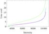 |
Fig. 1 Illustration of method used in this work to relate the line cord level to the corresponding line residual intensity (in arbitrary units). At each pixel along the spectrograph slit, the widths of the red and blue wings at a given residual intensity (red and blue curves respectively), are added to get the variation of the line cord width as a function of the residual line intensity (green curve). We then consider 25 line cord levels evenly distributed from the line center (level 1) to Δλc (see the text for the definition of Δλc). |
3. Cross-correlation of images
 |
Fig. 2 Reconstructed images of the granulation at three opacity levels in the 630.15 nm Fe i line. The geometrical scale is in arcseconds. Left panel: image at continuum level. Middle panel: image at line-center level. Right panel: image at line cord index 6 (close to the contrast inversion layer). Color code: the mean image intensity, Im is coded in black. The intensity range in each image is coded on 4 colors, showing respectively the levels [Im + (Imax − Im)/2;Imax] : red, [Im;Im + (Imax − Im)/2] : magenta, [Im − (Im − Imin)/2;Im] : cyan, [Im − (Im − Imin)/2;Imin] : blue. Imax and Imin denote respectively the maximum and minimum intensity in the image. The white circles show examples of structures exhibiting contrast inversion in the upper photosphere. |
Figure 2 shows an example of the reconstructed images obtained close to disk center at 3 line cord levels in the FeI 630.1 nm, namely at line center (level 1), close to the continuum (level 25), and at level 6, where the contrast inversion takes place. The color code shows the brightness level with respect to the average image intensity (coded in black), as explained in the figure caption. It is a relative scale aimed at enhancing the image contrast despite of the average intensity decrease from the continuum level to the line core levels. The brightest parts in each image are coded in red, and the darkest ones in blue. We remark that not all the granules visible at the continuum levels show contrast inversion in the line core image. However we shall see that the contrast inversion is a statistically significant phenomenon, which gives rise to a detectable negative peak in the cross-correlation of continuum and line core images.
We also show in Fig. 3, an image of vertical cuts of the photosphere, for three positions of the spectrograph slit. The intensity in the photosphere at the 25 continuum opacity levels was recovered with the procedure described above. Let us remark that the vertical axis in this figure does not show the geometrical height, but is related to the continuum optical depths where the intensities at the 25 levels are formed. In this paper we shall show how the perspective effect allows us to measure the geometrical height corresponding to level 1. We clearly see in Fig. 3 the contrast inversion layer as a dark line fluctuating between levels 7 and 10. We can notice that the contrast goes through a minimum in the contrast inversion layer. A forthcoming paper will be devoted to a detailed study of the depth-dependence of the photospheric mean intensity and rms-contrast.
 |
Fig. 3 Reconstructed images of the granulation at 25 continuum opacity levels, showing the depth-dependence of granular structures. Left panel: slit position at μ = 0.4 in the southern hemisphere, Central panel: slit position at disk center, Right panel: slit position at μ = 0.4 in the northern hemisphere. Color code: as in Fig. 2. |
3.1. Correlations and cross-correlations
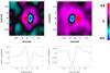 |
Fig. 4 2D cross-correlation of the images at line center and at the continuum level for μ = 0.3, in the northern hemisphere (left panel) and in the southern hemisphere (right panel). The south-north direction is along the horizontal axis. Lower left and right panels: south-north cuts, IC(τ), of the cross-correlations shown in the upper panels. |
Figure 4 shows an example of the cross-correlation of the images at line center and at the continuum level, for observations performed out of disk center, in the southern hemisphere and at a symmetrical position in the northern hemisphere. We notice that the image cross-correlation shows two peaks, one positive peak at the origin and a negative peak shifted with respect to the origin. In the following we denote by δ the distance, in arcseconds, between the origin and the minimum of the negative peak.
Let us now explain the origin of these peaks. We may assume that the images are the sum
of the granular structures and of a background, i.e. 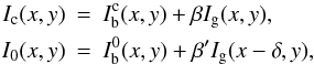 (3)where
Ic and I0 denote respectively
the continuum and line core image, Ig is the granulation
structure,
(3)where
Ic and I0 denote respectively
the continuum and line core image, Ig is the granulation
structure,  and
and
 denote the
background large scale structures in the continuum and line core images respectively. The
x coordinate is taken along the north-south direction. The average
image intensity is set to zero, so the coefficients β and
β′ are related to the contrast of the granulation;
β′ is negative in images where the granulation contrast is
inverted. In writting Eq. (3) we have
assumed that the granular structures seen at the line core level are identical to the ones
seen at the continuum level, except for the contrast inversion, but radially shifted by a
systematic effect. The cross-correlation is easily computed as the inverse Fourier
transform of the cross-spectrum. The cross-spectrum is given by
denote the
background large scale structures in the continuum and line core images respectively. The
x coordinate is taken along the north-south direction. The average
image intensity is set to zero, so the coefficients β and
β′ are related to the contrast of the granulation;
β′ is negative in images where the granulation contrast is
inverted. In writting Eq. (3) we have
assumed that the granular structures seen at the line core level are identical to the ones
seen at the continuum level, except for the contrast inversion, but radially shifted by a
systematic effect. The cross-correlation is easily computed as the inverse Fourier
transform of the cross-spectrum. The cross-spectrum is given by 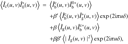 (4)and
the spectrum of the line core image is given by
(4)and
the spectrum of the line core image is given by  (5)The
brackets denote the ensemble average over a large number of structures. Assuming that the
granulation is not correlated with the background structures, the averages of the the
cross-terms in Eqs. (4) and (5) are on the form
(5)The
brackets denote the ensemble average over a large number of structures. Assuming that the
granulation is not correlated with the background structures, the averages of the the
cross-terms in Eqs. (4) and (5) are on the form
 , and
, and
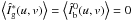 . We thus obtain
  (6)The
auto-correlation of the line core image may be considered as the sum of the background
auto-correlation and of the auto-correlation of the granulation. We notice that the order
of magnitude of the second term is given by the square of the granulation contrast which
is much smaller than unity. In the cut shown in Fig. 5 the contribution due to the granulation autocorrelation is added to the
dominant background peak. The cross-correlation is the sum of a positive peak and of a
negative peak which is shifted in the radial direction (a phase term is the Fourier space
corresponds to a shift in the real space). We notice that the order of magnitude of the
negative term is given by the product of the granulation contrast at the continuum level
and at the line core level. As a consequence the amplitude of the negative peak decreases
when one considers line levels closer to the contrast inversion layer, where the contrast
decreases to a few percents only.
(6)The
auto-correlation of the line core image may be considered as the sum of the background
auto-correlation and of the auto-correlation of the granulation. We notice that the order
of magnitude of the second term is given by the square of the granulation contrast which
is much smaller than unity. In the cut shown in Fig. 5 the contribution due to the granulation autocorrelation is added to the
dominant background peak. The cross-correlation is the sum of a positive peak and of a
negative peak which is shifted in the radial direction (a phase term is the Fourier space
corresponds to a shift in the real space). We notice that the order of magnitude of the
negative term is given by the product of the granulation contrast at the continuum level
and at the line core level. As a consequence the amplitude of the negative peak decreases
when one considers line levels closer to the contrast inversion layer, where the contrast
decreases to a few percents only.
Let us now describe how we measure the shift δ. We consider the
south-north cuts of the autocorrelations and cross-correlations, that we write on the form
 (7)where
 denotes the cross-correlation between the backgrounds of the continuum and line center
images, which is centered at zero, and ICg is
the cross-correlation peak of the granulation in both images, it is centered at
δ. The measurement of δ cannot be made directly by
measuring the distance between the positive and negative peaks because the two peaks are
blended. The wings of the positive peak partly overlap the negative peak, as a result the
shape of the negative peak is distorted and the location of its apparent minimum is
shifted.
denotes the cross-correlation between the backgrounds of the continuum and line center
images, which is centered at zero, and ICg is
the cross-correlation peak of the granulation in both images, it is centered at
δ. The measurement of δ cannot be made directly by
measuring the distance between the positive and negative peaks because the two peaks are
blended. The wings of the positive peak partly overlap the negative peak, as a result the
shape of the negative peak is distorted and the location of its apparent minimum is
shifted.
But we have noticed that it is possible to eliminate the positive peak, ICb(τ), simply by subtracting from IC(τ) a small fraction α of the correlation C(τ). This means that the correlation peak has approximately the same shape as the positive peak in the cross-correlation. The reason is probably that the background structures do not vary significantly from the low to the upper photosphere. This is illustrated in Fig. 5, where we show an example of the behaviour of IC(τ) for images recorded at μ = 0.82, in the continuum and at line cord level 5 in the FeI 603.1 nm line, i.e. close to the contrast inversion layer. We show that the positive peak may be rather well eliminated by subtrating from IC(τ) a fraction α of the auto-correlation of the line cord image. We then determine the location of the negative peak by fitting it with a 6th order polynomial. Let us notice however that the correction of the blend is not perfect, so that some errors on δ are introduced by this correction procedure. But we shall see in the following that the measurements performed on a large number of images show very little dispersion, this indicates that the method is quite robust and reliable.
 |
Fig. 5 Illustration of the subtraction of the positive peak from the cross-correlation. Left panel: north-south cut of the cross-correlation, IC(τ), of the image at line cord level 5 in the FeI line at 603.15 nm, with the image at the continuum level, for μ = 0.82. The negative peak of cross-correlation arising from the contrast inversion of the images is partly blended with the positive peak. Right panel: result of the subtraction IC(τ) − αC(τ), with α = 0.12. We notice the shift of the negative peak when the correction is applied. |
To test it further, we have computed the difference between the two curves obtained at line centers (top panels of Figs. 6 and 7). The difference is weakly dependent on μ and varies between 0.7 and 0.15 arcsec. This compares very well to the formation height difference that we measured directly in a previous work, using the cross-spectrum phase of granulation images obtained in the two lines (Faurobert et al. 2009). This previous differential method yields on the average a difference of formation heights between 63 km and 75 km in the quiet Sun. In this previous work we did not measure the line core formation-depths that we are now able to measure as we explain now.
3.2. Center-to-limb variations of the measured shifts
Figures 6 and 7 show the shifts we have measured in arc seconds, divided by sinθ, where θ is the heliocentric angle, for the two lines of the FeI 630 nm line pair and for the 160 positions along the south-north polar axis. Let us notice that the division with sinθ amplifies the dispersion of the measurements close to disk center where θ is very small (we go down to sinθ ≃ 10-2). In order to put the center of the solar disk at the origin, and to show both hemispheres, the results obtained in the southern hemisphere are shown as a function of −(1 − μ) (μ = cosθ) and the ones obtained in the northern hemisphere as a function of 1 − μ. The measurement is set to zero in cases where the contrast inversion is not detected. We observe that there is no more contrast inversion at line levels larger than 7 in the FeI 630.1 nm line and larger than 6 in the weaker 630.2 nm line. The contrast inversion is never detected close to the solar limb, for cosθ < 0.25. The reason is that, when observed close to the solar limb, continuum images are formed above the granulation contrast inversion layer. We notice the nice overall symmetry between the results obtained in the northern and southern hemispheres. We also notice that the measurements show a remarkably low dispersion. They are more scattered when one approaches the center of the solar disk, where the perspective effect vanishes, but we are still able to make consistent measurements very close to disk center. The measurements are also more scattered when one approaches the contrast inversion layer, because the accuracy of the measurement decreases when the image contrast decreases. We can perform consistent measurements down to the line cord level 5 in the FeI 630.1 nm line and level 4 in the 630.2 nm one.
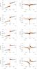 |
Fig. 6 Measurement of the FeI 630.1 nm line core formation depth δ/sinθ (θ denotes the heliocentric angle). Left column, from top panel to bottom panel: center-to-limb variations of the formation depth of the images at line cord levels 1 to 5 (orange dots), and their linear fit with the a and b coefficients given in Table 1 (black dots). Right column: difference between the measured values of δ/sinθ and their linear fit (orange dots) and analytical fit of this difference with the c and d coefficients given in Table 1 (black dots). Results obtained in the southern hemisphere (denoted by S on the figures) are shown as functions of the variable −1 + μ, whereas results obtained in the northern hemisphere (denoted by N) are shown are as functions of 1 − μ. |
In the following we interpret the observed shift as the result of two effects, namely, a perspective effect due to the continuum and line core formation-depth difference, and a true horizontal displacement of granules due to horizontal velocity fields. Mainly two kinds of velocitiy fields may induce detectable shifts of the structures between the low and upper photosphere, namely the expansion velocities of rising granules and large scale velocity fields at the supergranular scale. Expansion of granules, when observed close to disk center, are likely to induce almost symmetrical displacements towards the north and the south, which compensate statistically, whereas, when observed close to the limb, a net displacement may remain. On the other hand, large scale supergranular flows induce horizontal displacements which cannot be seen on the images at the limb as they are perpendicular to the plane of the sky, but which may be detected close to the solar disk.
Best fit values, in arc seconds, of the parameters a, b, c and d for both lines of the FeI 630 nm pair.
So we write  (8)where the first
term is the perspective shift and the second term is the true displacement of a granular
structure along the solar surface projected on the plane of the sky. The line cord
formation depth is denoted by h,
v// denotes the
component of the velocity parallel to the solar surface and τg
denotes the life-time of a granular structure. Equation (8) means that a granular structure embedded in a horizontal velocity
field with a vertical gradient would be observed at the altitude h with
an horizontal shift due to its advection during the life-time of the structure, by the net
horizontal velocity
(8)where the first
term is the perspective shift and the second term is the true displacement of a granular
structure along the solar surface projected on the plane of the sky. The line cord
formation depth is denoted by h,
v// denotes the
component of the velocity parallel to the solar surface and τg
denotes the life-time of a granular structure. Equation (8) means that a granular structure embedded in a horizontal velocity
field with a vertical gradient would be observed at the altitude h with
an horizontal shift due to its advection during the life-time of the structure, by the net
horizontal velocity  . We
propose to distinguish the perspective effect from the horizontal velocity effects by
looking at the center-to-limb variations of our measurements.
. We
propose to distinguish the perspective effect from the horizontal velocity effects by
looking at the center-to-limb variations of our measurements.
3.2.1. Line formation depth
The line formation height is expected to increase towards the limb because the
line-of-sight crosses higher regions of the photosphere. Here we assume that
h varies linearly with μ. The displacements due to
horizontal velocity gradients are discussed in more details in the next section. In
order to fit both the effect of the horizontal velocities of expanding rising granules
which can be observed close to the limb, and the effects of large scale horizontal
velocities visible close to disk center, we also fit the center-to-limb variations of
with a linear function of μ.
The linear regime of variation of
δ/sinθ related to the
center-to-limb variations of the line formation height, is clearly observed in Figs.
6 and 7. We
also notice that some departures to the linear regime appear mainly on measurements
performed close to disk center and that these departures tend to increase at line levels
formed deeper in the photosphere, closer to the inversion layer. At these levels we also
observe some departure to the linear regime close to the limb. We fit the linear regime
with the linear function a + bμ on the interval
0.4 < μ < 0.8, where
the two parameters a and b are obtained by a
least-square method, independently in the north and south hemispheres. Their values are
given in Table 1, for the two lines of the FeI
630 nm pair. Figures 6 and 7 also show the difference between the measurements of
δ/sinθ and the best linear fit.
Ascribing these differences to horizontal velocity effects we model them with the
analytical expression  ,
and we determine the values of the parameters c and d
by least square fitting on the interval
0.25 < μ < 0.95. We
do not consider the measurements performed closer to disk center, where the dispersion
is quite large. The values of c and d are given in
Table 1. The quality of the fits is illustrated
in Figs. 6 and 7. Let us notice that this “two-step” fitting procedure allows us to better
model the linear regime of center-to-limb variations, by restricting its validity domain
to an interval excluding both limb and disk center regions.
,
and we determine the values of the parameters c and d
by least square fitting on the interval
0.25 < μ < 0.95. We
do not consider the measurements performed closer to disk center, where the dispersion
is quite large. The values of c and d are given in
Table 1. The quality of the fits is illustrated
in Figs. 6 and 7. Let us notice that this “two-step” fitting procedure allows us to better
model the linear regime of center-to-limb variations, by restricting its validity domain
to an interval excluding both limb and disk center regions.
We recall that a positive shift corresponds to a displacement towards the north pole. The perspective shift is towards the north pole in the northern hemisphere and towards the south pole in the southern hemisphere. We derive the line formation heights from the values of the parameters a and b at line centers. Averaging the shifts obtained in the northern and southern hemispheres, we find that the formation-depth of the FeI 630.1 nm line varies from 0.32 arcsec (230 km), at disk center, to 0.79 arcsec (580 km), at μ = 0.25. For the FeI 630.2 nm line, we find that the line center image is formed at an altitude of 0.27 arcsec (200 km), at disk center, and of 0.64 arcsec (470 km) at μ = 0.25.
In Grec et al. (2010), we performed 3D radiative transfer calculations in these two lines and we could simulate the images of the solar photosphere at line centers using a 3D numerical model of the photospheric magneto-convection. Then we derived the line formation heights by measuring the perspective shift of the simulated images on a line-of-sight at μ = 0.87. These simulations give results which are quite close to what we measure here on the real Sun, namely we obtained 270 km for the FeI line at 630.1 nm and 200 km for the 630.2 nm line. Let us notice that this is however quite different from the heights where the optical depth at line centers is equal to one, derived, for example, in Shchukina & Trujillo Bueno (2001).
The measurements that we perform here at lines-of-sight closer to the limb can be used to test the 3D numerical simulations of the upper layers of the photosphere, where the convection overshooting vanishes. We find that the line formation heights increase significantly towards the limb, reaching 580 km at μ = 0.25 for the FeI 630.1 nm line. Such a large value is not expected from the current 3D numerical simulations of the photosphere (Uitenbroek 2011, priv. comm.). This discrepancy indicates that simulations have to be improved to better account for the physics in the upper layers of the photosphere.
3.2.2. Effect of horizontal velocities
The true displacements due to horizontal velocities can be detected when they are on the same order of magnitude, or larger than the perspective shift. Let us now estimate the order of magnitude of velocities which can induce shifts on the same order as the perspective shift. The condition is hsinθ ≃ h(∂v///∂z)τgcosθ. With ∂v///∂z ≃ Δv///h, where Δv// is the variation of the horizontal velocity on the height h, we finally get Δv// ≃ h/τg(sinθ/cosθ). The mean life-time of granular structures is τg ≃ 600 s (Roudier et al. 2012), so by using h ≃ 0.3′′ (the average formation height measured at line centers), we obtain as an order of magnitude, Δv// ≃ 360(sinθ/cosθ) m/s. So close to disk center, measurable displacements are induced by horizontal velocity fields with relatively small depth gradients (typically on the order or smaller than 360 m/s over the line formation height for lines-of-sight at μ > 0.7), whereas close to the solar limb, only large horizontal velocity gradients may induce detectable horizontal displacements (typically larger than 600 m/s over the line formation height for lines-of-sigth at μ < 0.5). So supergranular horizontal velocity fields are likely to affect the displacements measured close to disc center, as their gradients are on the required order of magnitude (Roudier et al. 2012), and horizontal granular velocities of expanding granules may affect the displacements measured close to the solar limb. Let us stress however, that we do not intend here to measure accurately the horizontal velocities which affect our observations. This is not possible because the method we are using is not suitable for this purpose.
First we measure shifts in the south-north direction only, so that we can only detect displacements towards the poles or the equator. Furthermore, we recall that we perform a statistical study of the granulation, which is valid because we observe a large number of granular structures. So, we do not actually follow any individual granule as it is advected by horizontal flows in the photosphere, but the statistical result of a large number of individual motions. Supergranular flows affect our measurements because they are organized on large horizontal scales (50′′ × 50′′), as compared to the typical size of a granule and on large time scales, as compared to the life-time of granules. The size of the images we analyze (20′′ × 60′′) is not large enough to average out the effect of supergranular flows but too large to measure properly its velocities. As for the effects of the horizontal expansion of rising granules which would be seen on individual granules at the limb, they are averaged out in our statistical study, so that they do not affect the shifts we are measuring close to the limb. This is shown in Figs. 6 and 7 where the linear fit is still valid close to the limb. Due to these statistical averaging both the parameters c and d of our analytical model take very small values.
3.3. Remark on the effect of quiet Sun magnetic fields
The FeI line pair at 630 nm is sensitive to the Zeeman effect of magnetic fields. In the quiet Sun, strong mainly vertical magnetic fields are present in small magnetic elements concentrated in the intergranular lanes and forming the magnetic network. Inside the network, the magnetic field appears as a mixed polarity field with random orientation and a much smaller strength on the order of a few tens of Gauss (Bommier et al. 2009; Bommier 2011). Mixed polarity weak fields do not give rise to a measurable Zeeman effect in the observations that we are analyzing here, we have checked this on the data, as SOT/SP provides Stokes spectra profiles for the same observing run. Zeeman polarization is detected only in small network elements. Actually, the Zeeman effect of small magnetic fields with mixed polarity over the resolution element affects the line absorption profile both by slightly broadening it and by reducing the line strength r. However, as the Zeeman splitting remains much smaller than the local Doppler width, this is a second order effect as compared to the effects of granular motions and temperature fluctuations. In the network elements where Zeeman polarization is detected, magnetic effects on the line formation depth are more important, as shown for example in Faurobert et al. (2009). But these
regions cover a small fraction of our (20′′ × 60′′) images, so they play a negligible role in the statistical study that we have performed here. It would be interesting to perform the same cross-correlation analysis on a statistical sample of magnetic network patches in order to measure the line formation depth in these structures.
4. Conclusion
The cross-correlation between images of the photospheric granulation taken at different line cords in the cores of the FeI 630 nm line pair shows a negative anti-correlation peak due the contrast inversion of the granulation in the upper photosphere. When observed out of disk center, the negative peak is shifted both because of the perspective effect and of the horizontal displacement of granular structures by horizontal flows with depth gradients. The two effects may be distinguished because they have different center-to-limb variations. We derive the line formation heights by measuring the perspective shift at line centers. For the FeI 630.1 nm line, the formation height varies from 230 km at disk center (200 km for the 630.2 nm line), to 580 km (470 km for the 630.2 nm line), at cosθ = 0.25. At small heliocentric angles, these results are in very good agreement with the 3D-numerical simulations that we performed previously for these two lines (Grec et al. 2010), but at larger heliocentric angles, we measure larger formation heights than predicted by 3D simulations. This confirms the validity of 3D numerical simulations of magneto-convection in the low layers of the photosphere, but this also points out that the physics of the upper-photosphere is still not modeled accurately enough to provide us with quantitative estimates of the line formation processes. As we observe the contrast inversion at the center of the FeI 630.2 nm line, we can safely conclude that the altitude where the contrast inversion of the granulation takes place is smaller than 200 km. The method that we have developed here may be applied to any spectral line formed under LTE conditions in the photosphere. However it requires 2D spectroscopic data with good spatial and spectral resolution.
References
- Asplund, M., Nordlund, Å., Trampedach, R., Allen de Prieto, C., & Stein, R. F. 2000, A&A, 359, 729 [NASA ADS] [Google Scholar]
- Bommier, V. 2011, A&A, 530, A51 [NASA ADS] [CrossRef] [EDP Sciences] [Google Scholar]
- Bommier, V., Martínez González, M., Bianda, M., et al. 2009, A&A, 506, 1415 [NASA ADS] [CrossRef] [EDP Sciences] [Google Scholar]
- Cheung, M. C. M., Schüssler, M., & Moreno-Insertis, F. 2007, A&A, 461, 1163 [NASA ADS] [CrossRef] [EDP Sciences] [Google Scholar]
- Faurobert, M., Aime, C., Périni, C., et al. 2009, A&A, 507, L29 [NASA ADS] [CrossRef] [EDP Sciences] [Google Scholar]
- Grec, C., Uitenbroek, H., Faurobert, M., & Aime, C. 2010, A&A, 514, A91 [NASA ADS] [CrossRef] [EDP Sciences] [Google Scholar]
- Kostik, R., Khomenko, E., & Shchukina, N. 2009, A&A, 506, 1405 [NASA ADS] [CrossRef] [EDP Sciences] [Google Scholar]
- Roudier, T., Rieutord, M., Malherbe, J. M., et al. 2012, A&A, 540, A88 [NASA ADS] [CrossRef] [EDP Sciences] [Google Scholar]
- Shchukina, N., & Trujillo Bueno, J. 2001, ApJ, 550, 970 [NASA ADS] [CrossRef] [Google Scholar]
- Stein, R. F., & Nordlund, A. 1998, ApJ, 499, 914 [Google Scholar]
- Stein, R. F., & Nordlund, Å. 2006, ApJ, 642, 1246 [NASA ADS] [CrossRef] [Google Scholar]
- Wedemeyer-Böhm, S., & Rouppe van der Voort, L. 2009, A&A, 503, 225 [NASA ADS] [CrossRef] [EDP Sciences] [Google Scholar]
All Tables
Best fit values, in arc seconds, of the parameters a, b, c and d for both lines of the FeI 630 nm pair.
All Figures
|
Fig. 1 Illustration of method used in this work to relate the line cord level to the corresponding line residual intensity (in arbitrary units). At each pixel along the spectrograph slit, the widths of the red and blue wings at a given residual intensity (red and blue curves respectively), are added to get the variation of the line cord width as a function of the residual line intensity (green curve). We then consider 25 line cord levels evenly distributed from the line center (level 1) to Δλc (see the text for the definition of Δλc). |
| In the text | |
|
Fig. 2 Reconstructed images of the granulation at three opacity levels in the 630.15 nm Fe i line. The geometrical scale is in arcseconds. Left panel: image at continuum level. Middle panel: image at line-center level. Right panel: image at line cord index 6 (close to the contrast inversion layer). Color code: the mean image intensity, Im is coded in black. The intensity range in each image is coded on 4 colors, showing respectively the levels [Im + (Imax − Im)/2;Imax] : red, [Im;Im + (Imax − Im)/2] : magenta, [Im − (Im − Imin)/2;Im] : cyan, [Im − (Im − Imin)/2;Imin] : blue. Imax and Imin denote respectively the maximum and minimum intensity in the image. The white circles show examples of structures exhibiting contrast inversion in the upper photosphere. |
| In the text | |
|
Fig. 3 Reconstructed images of the granulation at 25 continuum opacity levels, showing the depth-dependence of granular structures. Left panel: slit position at μ = 0.4 in the southern hemisphere, Central panel: slit position at disk center, Right panel: slit position at μ = 0.4 in the northern hemisphere. Color code: as in Fig. 2. |
| In the text | |
|
Fig. 4 2D cross-correlation of the images at line center and at the continuum level for μ = 0.3, in the northern hemisphere (left panel) and in the southern hemisphere (right panel). The south-north direction is along the horizontal axis. Lower left and right panels: south-north cuts, IC(τ), of the cross-correlations shown in the upper panels. |
| In the text | |
|
Fig. 5 Illustration of the subtraction of the positive peak from the cross-correlation. Left panel: north-south cut of the cross-correlation, IC(τ), of the image at line cord level 5 in the FeI line at 603.15 nm, with the image at the continuum level, for μ = 0.82. The negative peak of cross-correlation arising from the contrast inversion of the images is partly blended with the positive peak. Right panel: result of the subtraction IC(τ) − αC(τ), with α = 0.12. We notice the shift of the negative peak when the correction is applied. |
| In the text | |
|
Fig. 6 Measurement of the FeI 630.1 nm line core formation depth δ/sinθ (θ denotes the heliocentric angle). Left column, from top panel to bottom panel: center-to-limb variations of the formation depth of the images at line cord levels 1 to 5 (orange dots), and their linear fit with the a and b coefficients given in Table 1 (black dots). Right column: difference between the measured values of δ/sinθ and their linear fit (orange dots) and analytical fit of this difference with the c and d coefficients given in Table 1 (black dots). Results obtained in the southern hemisphere (denoted by S on the figures) are shown as functions of the variable −1 + μ, whereas results obtained in the northern hemisphere (denoted by N) are shown are as functions of 1 − μ. |
| In the text | |
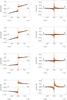 |
Fig. 7 Same as Fig. 6, for levels 1 to 4 in the FeI 630.2 nm line. |
| In the text | |
Current usage metrics show cumulative count of Article Views (full-text article views including HTML views, PDF and ePub downloads, according to the available data) and Abstracts Views on Vision4Press platform.
Data correspond to usage on the plateform after 2015. The current usage metrics is available 48-96 hours after online publication and is updated daily on week days.
Initial download of the metrics may take a while.