| Issue |
A&A
Volume 548, December 2012
|
|
|---|---|---|
| Article Number | A44 | |
| Number of page(s) | 16 | |
| Section | Planets and planetary systems | |
| DOI | https://doi.org/10.1051/0004-6361/201219337 | |
| Published online | 16 November 2012 | |
A study of the performance of the transit detection tool DST in space-based surveys
Application of the CoRoT pipeline to Kepler data
1
Institute of Planetary Research, German Aerospace Center,
Rutherfordstrasse 2,
12489
Berlin, Germany
e-mail: This email address is being protected from spambots. You need JavaScript enabled to view it.
2
Center for Astronomy and Astrophysics, TU Berlin,
Hardenbergstr. 36, 10623
Berlin,
Germany
Received:
4
April
2012
Accepted:
24
September
2012
Abstract
Context. Transit detection algorithms are mathematical tools used for detecting planets in the photometric data of transit surveys. In this work we study their application to space-based surveys.
Aims. Space missions are exploring the parameter space of the transit surveys where classical algorithms do not perform optimally, either because of the challenging signal-to-noise ratio of the signal or its non-periodic characteristics. We have developed an algorithm addressing these challenges for the mission CoRoT. Here we extend the application to the data from the space mission Kepler. We aim at understanding the performances of algorithms in different data sets.
Methods. We built a simple analytical model of the transit signal and developed a strategy for the search that improves the detection performance for transiting planets. We analyzed Kepler data with a set of stellar activity filtering and transit detection tools from the CoRoT community that are designed for the search of transiting planets.
Results. We present a new algorithm and its performances compared to one of the most widely used techniques in the literature using CoRoT data. Additionally, we analyzed Kepler data corresponding to quarter Q1 and compare our results with the most recent list of planetary candidates from the Kepler survey. We found candidates that went unnoticed by the Kepler team when analyzing longer data sets. We study the impact of instrumental features on the production of false alarms and false positives. These results show that the analysis of space mission data advocates the use of complementary detrending and transit detection tools also for future space-based transit surveys such as PLATO.
Key words: planetary systems / techniques: polarimetric
© ESO, 2012
1. Introduction
Transit detection algorithms are mathematical tools that aim at detecting the signal of a transiting planet in the photometric time series of a star (light curve). The generally accepted characteristics of the planet transit are a short, small, periodic decrease of the (assumed) constant luminosity flux of the star caused by the interposition of the opaque planet in front of the stellar disk, as seen from the point of view of the observer. Transits are short because the duration of a transit is roughly proportional to the quotient of the radius of the star over the semi-major axis of the orbit of the planet (tT/P ~ R∗/πa; see Seager & Mallén-Ornelas 2003). This means that even for the shortest known period exoplanets orbiting at 3 or 4 stellar radii, such as 55 Cnc e (Winn et al. 2011), WASP-19b (Hebb et al. 2010), WASP-43b (Hellier et al. 2011), Kepler-10b (Batalha et al. 2011), CoRoT-7b (Léger et al. 2009), or WASP-18b (Hellier et al. 2009) (all of them with orbital periods shorter than 24 h) the duration is shorter than one tenth of the orbital period. Transit depths are small because the diminution of the flux is proportional to the square of the quotient of the radii of the planet and the star: ΔF/F ~ (Rp/R∗)2.
The arrival of space-based surveys of exoplanets such as CoRoT (Baglin et al. 2006) and Kepler (Borucki et al. 2010) has placed transit surveys in the region of the parameter space where transits are not short, in terms of hours, any more. For example, the transit of CoRoT-9b (Deeg et al. 2010) lasts 8 h, but there are also detections of giant eclipsing binaries where the eclipses last several days, like CoRoT 101126445, whose eclipses last 49 h for a period of 30 days (Cabrera et al. 2009). At the same time, the detected signals are not weak either. In this case there are two tendencies, on the one hand toward really shallow transits, such as those of the terrestrial planets 55 Cnc e, CoRoT-7b or Kepler-10b, and on the other hand toward transits of small planets around small stars, which enables detecting Earth-sized planets from the ground, such as GJ-1214b (Charbonneau et al. 2009). Finally there are detections of transits that are not periodic anymore, the transit timing variations of Kepler-9c (Holman et al. 2010) reach an amplitude of 140 min, comparable with the length of the transit, in a time span of 200 days.
Space surveys of transiting planets such as CoRoT and Kepler have improved our knowledge about the performances of transit detection techniques. Between 2004 and 2007 the CoRoT community made a series of studies to test the transit detection capabilities of different algorithms. The analysis of the results of these tests, published by Moutou et al. (2005, 2007), revealed on the one hand that all algorithms had competitive performances and yielded comparable results, but on the other hand it was shown that both false alarms and non-detections were method dependent. The transit detection approach followed by the CoRoT community is based on the results of these analyses: combine the results of different teams using different detrending and detection techniques to reduce the rate of false alarms and to push the detection limit as far as possible.
The Kepler survey has followed a different approach using one single detrending and detection algorithm (Jenkins 2002; Jenkins et al. 2010b) whose performance has been extensively studied and tested (Jenkins et al. 2002, 2010a). In view of future transit search missions, e.g. PLATO (Catala 2009), it is interesting to compare the different approaches.
There are several tools in the literature dealing with the automatic detection of transiting candidates (Aigrain & Favata 2002; Bonomo & Lanza 2008; Bordé et al. 2007; Carpano & Fridlund 2008; Collier Cameron et al. 2006; Defaÿ et al. 2001; Grziwa et al. 2012; Jenkins et al. 1996; Jenkins 2002; Kovács et al. 2002; Ofir 2008; Protopapas et al. 2005; Régulo et al. 2007; Renner et al. 2008; Schwarzenberg-Czerny & Beaulieu 2006). In addition to those, Schwarzenberg-Czerny (1998) gives a very interesting discussion on the general techniques for the detection of periodic signals.
The code presented in this paper has been used regularly since 2006 in the CoRoT survey for transiting planets (Carpano et al. 2009; Cabrera et al. 2009; Erikson et al. 2012; Carone et al. 2012; Cavarroc et al. 2012). The algorithm, called Détection Spécialisée de Transits (DST) addresses some of the challenges that face current and future transit surveys. This algorithm aims at a specialized detection of transits by improving the consideration of the transit shape and the presence of transit timing variations. As a first step, we have applied our CoRoT detrending and transit detection tools to the public data release Q1 (Borucki et al. 2011a) and compared the results to the list of planetary candidates published by Kepler (Borucki et al. 2011b, hereafter B11b; Batalha et al. 2012). We aim at testing the capabilities of a different algorithm to find new transit candidates in a reduced data set, because we also aim at understanding the dependence of the yield as a function of the length of the observations. Such a study was already started in CoRoT (Cabrera et al. 2009) and it is of great interest when deciding the observation strategy of transit surveys, for example when deciding the optimimum length of an observational run. On the other hand, it is important to find successful algorithms that are able to detect planets in data sets with a reduced number of transit events. This is the case of modern transit surveys aiming at detecting planetary candidates with periods comparable to the total length of the observations, for example planets in the habitable zone of solar-like stars.
Section 2 contains the mathematical description of the algorithm. Section 3 compares the performance of the new algorithm with a widely used technique, the BLS code (Kovács et al. 2002). We do not aim to reproduce the algorithm comparisons found in the literature such as the analysis made by Tingley (2003a,b) or Moutou et al. (2005, 2007) but to present the differences of this new code with respect to one of the most widely used codes (BLS) and explain its advantages. Section 6 describes the treatment applied to Kepler Q1 data. Section 7 describes the results of the test, including a number of new transiting candidates. Finally, Sect. 8 summarizes the outcome and describes future developments.
2. The transit search algorithm
A light curve is a time series of the photometric observations of a star. Mathematically,
it can be seen as a collection of pairs of time-flux, which can be translated into a
function like 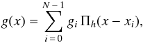 (1)where
(xi,gi)
are the N pairs time-flux and
(1)where
(xi,gi)
are the N pairs time-flux and 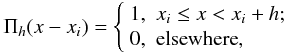 (2)with h being the integration
time. g(x) should not be understood as the function
representing the continuous time waveform corresponding to the photometric measurement, but
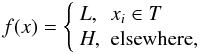
as a mathematical tool to represent photometric observations. If
G(t) represents the continuous waveform coming from the
star, gi is defined as
(2)with h being the integration
time. g(x) should not be understood as the function
representing the continuous time waveform corresponding to the photometric measurement, but
as a mathematical tool to represent photometric observations. If
G(t) represents the continuous waveform coming from the
star, gi is defined as 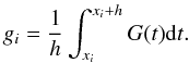 (3)The BLS (Kovács
et al. 2002) is arguably the most popular transit detection algorithm in the
literature. It proposes a box model for the transit shape, which can be described as
(3)The BLS (Kovács
et al. 2002) is arguably the most popular transit detection algorithm in the
literature. It proposes a box model for the transit shape, which can be described as
 (4)where H is the mean value of
the flux out of transit and H − L is the depth of the
transit, which occurs in the interval T. The test statistic defined by BLS
is the distance between the functions f and g, defined as
(4)where H is the mean value of
the flux out of transit and H − L is the depth of the
transit, which occurs in the interval T. The test statistic defined by BLS
is the distance between the functions f and g, defined as
 (5)where we have defined the weight function
analogously to g
(5)where we have defined the weight function
analogously to g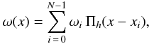 (6)keeping the definition of Kovács et al. (2002):
 ![Mathematical equation: \hbox{$\omega_i = \sigma_i^{-2} \linebreak \left[ \sum_{j\,=\,0}^{N\,-\,1} \sigma_j^{-2} \right]^{-1}$}](/articles/aa/full_html/2012/12/aa19337-12/aa19337-12-eq20.png) . It is trivial to prove that (5) is the product of the constant
h (the integration time) times the test statistic defined by Eq. (1) in
Kovács et al. (2002). Expression (5) can be minimized analytically with respect to
the variables H and L once the transit region
T is known:
. It is trivial to prove that (5) is the product of the constant
h (the integration time) times the test statistic defined by Eq. (1) in
Kovács et al. (2002). Expression (5) can be minimized analytically with respect to
the variables H and L once the transit region
T is known: ![Mathematical equation: \begin{equation} \label{eq:BLS_H_L} H = \frcn{ \displaystyle \sum_{i\,=\,0}^{N\,-\,1} \omega_i g_i - \sum_{ i \in T} \omega_i g_i}{ \displaystyle \sum_{i\,=\,0}^{N\,-\,1} \omega_i - \sum_{ i \in T} \omega_i }, \\[1.2cm] L = \frcn{ \displaystyle \sum_{ i \in T} \omega_i g_i}{ \displaystyle \sum_{ i \in T} \omega_i }, \end{equation}](/articles/aa/full_html/2012/12/aa19337-12/aa19337-12-eq22.png) (7)and the BLS test statistic is
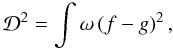
(7)and the BLS test statistic is ![Mathematical equation: \begin{equation} \label{eq:BLS_statistic_final} \mathcal{D}^2 = h \left[ \sum_{i\,=\,0}^{N\,-\,1} \omega_i g_i^2 - \frcn{ \left( \displaystyle \sum_{i\,=\,0}^{N\,-\,1} \omega_i g_i - \sum_{i \in T} \omega_i g_i \right)^2 }{ \displaystyle \sum_{i\,=\,0}^{N\,-\,1} \omega_i - \sum_{i \in T} \omega_i } - \frcn{ \left( \displaystyle \sum_{i \in T} \omega_i g_i \right)^2 }{ \displaystyle \sum_{i \in T} \omega_i } \right], \end{equation}](/articles/aa/full_html/2012/12/aa19337-12/aa19337-12-eq23.png) (8)which is further simplified by making
(8)which is further simplified by making
 and
and  this finally produces Eq. (4) in Kovács et al. (2002).
In practice, as the ephemeris of the transit (period P, epoch x0 and transit length d) are not known a priori, one folds and bins the light curve to a test period and then calculates the test statistic for every possible value of x0 and d. The minimum of the test statistic corresponds to the ephemeris of the transit. If there is no significant extreme value of the test statistic, the conclusion is that there is no detectable transit in the light curve at the tested period.
We can define an alternative model to the transit function using a parabola instead of a
box function and modifying the definition of the region in transit. The advantages of these
choices are shown in Sect. 3. The model function will
be 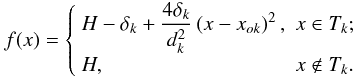 (9)We assume that there are K
observed transits, each transit denoted as Tk
centered in the position xok. The definition of
the transits is discussed in the next section. The duration of the kth
transit Tk is given by
dk and its depth by
δk. The definition of the distance between
the functions f and g is identical to (5) and its minimization with respect to the
variables H and δk yields the
following constraint:
(9)We assume that there are K
observed transits, each transit denoted as Tk
centered in the position xok. The definition of
the transits is discussed in the next section. The duration of the kth
transit Tk is given by
dk and its depth by
δk. The definition of the distance between
the functions f and g is identical to (5) and its minimization with respect to the
variables H and δk yields the
following constraint: ![Mathematical equation: \begin{equation} \label{eq:Dst_H_delta} H = \frcn{ \displaystyle \sum_{i\,=\,0}^{N\,-\,1} \omega_i g_i - \sum_{k} \frcn{\Lambda_k^2 g\Lambda_k^2}{\Lambda_k^4} }{ \displaystyle \sum_{i\,=\,0}^{N\,-\,1} \omega_i - \sum_{k} \frcn{\left(\Lambda_k^2\right)^2}{\Lambda_k^4} }, \\[1.4cm] \delta_k = \frcn{d_k^2}{4} \frcn{ g\Lambda_k^2 - H \Lambda_k^2}{\Lambda_k^4}, \end{equation}](/articles/aa/full_html/2012/12/aa19337-12/aa19337-12-eq36.png) (10)where
(10)where ![Mathematical equation: \begin{eqnarray} \label{eq:Dst_Lambdas} \Lambda_k^2 \displaystyle &&= \sum_{i \in T_k} \omega_i \left[ \left( x_i - x_{ok} + \frcn{h}{2} \right)^2 - \frcn{d_k^2}{4} + \frcn{h^2}{12} \right], \nonumber\\ g\Lambda_k^2 \displaystyle &&= \sum_{i \in T_k} \omega_i \left[ \left( x_i - x_{ok} + \frcn{h}{2} \right)^2 - \frcn{d_k^2}{4} + \frcn{h^2}{12} \right] g_i, \\ \Lambda_k^4 \displaystyle &&= \sum_{i \in T_k} \omega_i \left[ \left( x_i \! -\! x_{ok} \! +\! \frcn{h}{2} \right)^4 + \frcn{1}{2} \left( h^2 - d^2 \right) \left( x_i - x_{ok} - \frcn{h}{2} \right)^2 \right. \nonumber\\ &&\displaystyle \qquad \left.+ \frcn{1}{8} \left( \frcn{h^4}{10} - \frcn{d_k^2 h^2}{3} + \frcn{d_k^4}{2} \right) \right]\cdot \nonumber \end{eqnarray}](/articles/aa/full_html/2012/12/aa19337-12/aa19337-12-eq37.png) (11)Using the above constraints, the distance
between the functions f and g becomes
(11)Using the above constraints, the distance
between the functions f and g becomes ![Mathematical equation: \begin{equation} \label{eq:Dst_statistic} \mathcal{D}^2 = h \left[ \sum_{i\,=\,0}^{N\,-\,1} \omega_i g_i^2 - H \sum_{i\,=\,0}^{N\,-\,1} \omega_i g_i - \sum_{k} \frcn{4 \delta_k}{d_k^2} g\Lambda_k^2 \right]\cdot \end{equation}](/articles/aa/full_html/2012/12/aa19337-12/aa19337-12-eq38.png) (12)However, contrary to Kovács et al. (2002), we are not going to define the test statistic as
the distance between the functions f and g (or, in the
case of BLS, the signal residue resulting from subtracting the constant term
(12)However, contrary to Kovács et al. (2002), we are not going to define the test statistic as
the distance between the functions f and g (or, in the
case of BLS, the signal residue resulting from subtracting the constant term
 ) from (8). Following Schwarzenberg-Czerny
(1998), for a signal x that is decomposed into its model
x∥ and residuals
x⊥ = x − x∥, the
statistic used to assess if the model is an appropriate description of the data will be
||x∥||2/||x⊥||2,
where
) from (8). Following Schwarzenberg-Czerny
(1998), for a signal x that is decomposed into its model
x∥ and residuals
x⊥ = x − x∥, the
statistic used to assess if the model is an appropriate description of the data will be
||x∥||2/||x⊥||2,
where  . As indicated in the previously cited paper,
we can draw the same conclusions with other statistics provided that they are uniquely
related (see also Jenkins et al. 1996; Tingley 2003b; Schwarzenberg-Czerny & Beaulieu 2006). In our notation,
x = g
and x∥ = f,
whereas
. As indicated in the previously cited paper,
we can draw the same conclusions with other statistics provided that they are uniquely
related (see also Jenkins et al. 1996; Tingley 2003b; Schwarzenberg-Czerny & Beaulieu 2006). In our notation,
x = g
and x∥ = f,
whereas  therefore the statistic is
 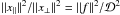 .
In this case
.
In this case 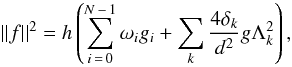 (13)and finally the test statistic is
 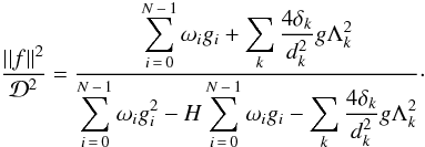 (14)
(14)
3. Discussion of the transit search algorithm
The test statistic defined by (14) is more complicated than defined by BLS (see 8) and hence it involves a heavier computational effort. However, it has four main advantages: 1) it provides a better description of the transit shape, which in turn provides a better behavior of the algorithm in the presence of transits; 2) it uses the same number of free parameters as BLS; it is always possible to improve the model of the transit shape by using more free parameters (for example, a trapezoid has one more free parameter: the duration of the ingress phase), but at the expense of computational effort; 3) our estimator performs better than BLS for the reasons explained below, and 4) the definition of the region in transit is more flexible.
To illustrate these assertions, we have analyzed public data from the satellite CoRoT1 with both BLS and the new method described in this paper (DST) and compared their performance in two test cases. In the first one (Sects. 3.1 and 3.2), we show how the DST model of the transit shape improves the transit detection efficiency. We have chosen two typical targets of transit surveys for this test, a planet, CoRoT-1b (Barge et al. 2008), and an eclipsing binary, CoRoT 102763847 (Carpano et al. 2009), of similar depths and durations, although different periods. We chose an eclipsing binary because although transit surveys aim at detecting planets, they find many eclipsing binaries as a by-product. The probability to detect eclipsing binaries is relatively higher because they are numerous and because the signal-to-noise ratio (S/N) of eclipses is in general stronger than the S/N of a planetary transit, since in stellar binary systems both members have in general comparable sizes. By choosing a planet and an eclipsing binary of similar depths and brightness we can compare the S/N of the detection in typical targets of planet detection surveys. Both targets were observed at the CoRoT sampling rates2 of 32 s and 512 s and the S/N achieved are representative of typical giant planet signals in transit surveys. This first test case consists of the analysis of a section of the light curve containing only one transit, respectively one eclipse. We implemented the BLS and DST algorithms3 and we applied them on the same data set to compare their performances.
But in addition to Jupiter planets, transit surveys also aim at detecting small terrestrial planets. In our second test case (Sect. 3.3) we compare the detectability with BLS and DST of CoRoT-7b, representative of the dim signals of Earth-sized planets. In this case we performed a blind search for the period of the transiting planet using the same filtered light curve for both algorithms.
3.1. Test case I: the transit shape
A second-order polynomial is expected to yield a better description of the transit shape than a box model because it includes a description, although incomplete, of the ingress and egress of the transit, which the box-shaped description simply ignores. The number of free parameters in DST and BLS is the same: the value of the flux out of transit H, the depth of the transit δk = H − L, and the ephemeris of the transit (period P, epoch x0, and duration d). This is in contrast to the trapezoidal model of the transit, which involves one more free parameter (the duration of the ingress phase). As we are analyzing the data of a single event, we fix the value of the period in the following analysis.
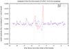 |
Fig. 1 Residuals of the BLS and DST model of CoRoT-1b sampled at 512 s. The central time of the transit chosen has a Julian Date value of 2 454 142.8547 days. The dotted vertical lines indicate the duration of the transit. |
We used the BLS and the DST algorithms to fit the aforementioned free parameters around the position of the chosen events. We show in Fig. 1 the residuals of the fit of the CoRoT-1b transit sampled at 512 s with BLS and DST. Figure 2 shows the same residuals for the 32 s sampling. These figures show that BLS fails to reproduce the transit shape in the ingress and egress, as expected. In Sect. 2 we have shown that the statistic used by BLS and DST is the distance between the observed data points and the model function as described by expression 5. Table 1 shows that DST is indeed a better description of the transit and eclipse signal. When the S/N is high (in the 512 s sampled ratio), DST produces 68% and 59% less residuals than BLS (for the planet and the eclipsing binary, respectively). When the S/N is lower (in the 32 s sampled ratio) the difference is less accentuated and DST performs around 14% better in both targets.
It might be rightfully argued that the parabolic is not the best description of the
flat bottom feature of planetary transits. Indeed, there are functions
that better reproduce the shape of long transits, where the contribution of the
flat part is most relevant, such as the cases of the already discussed
CoRoT-9b or, for an example of a super-Earth, Kepler-22b (Borucki et al. 2012). Figure 3 shows the
binned light curve of Kepler-22b modeled with the parabolic shape described in this paper
(labeled x2), with a quadratic shape (labeled
x4) described by Eq. (15) below, and with BLS. Indeed, Kepler-22b, a ~2 Earth radii
planet with an orbital period of 290 days is not a challenging detection for DST
considering the distinct signal produced by the planet in the periodogram (see Fig. 4) 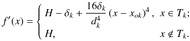 (15)If we compare the residuals of these models,
we immediately see that most of the residuals of BLS come from the ingress and egress
phases, as was the case with CoRoT-1b above. We can also verify that
the x4 model performs slightly better than
the x2 model, but we do not obtain the same degree of
improvement as when we compare x2 and BLS. Indeed, if
f(x) is the best function describing the shape of a
transit, and if this function is even (which is best true for circular orbits and
spherical stars), then the x2 model is the first non-null term
of the Taylor series of the optimal function f(x). In
some cases, the term in x4 might be more representative, but
it will always be a more complicated description and it will be far from optimal for
transits with higher impact parameters. The parabolic model is not the best model, but it
is the most simple (with fewer free parameters), analytic, continuous (in contrast to BLS)
description of the transit.
(15)If we compare the residuals of these models,
we immediately see that most of the residuals of BLS come from the ingress and egress
phases, as was the case with CoRoT-1b above. We can also verify that
the x4 model performs slightly better than
the x2 model, but we do not obtain the same degree of
improvement as when we compare x2 and BLS. Indeed, if
f(x) is the best function describing the shape of a
transit, and if this function is even (which is best true for circular orbits and
spherical stars), then the x2 model is the first non-null term
of the Taylor series of the optimal function f(x). In
some cases, the term in x4 might be more representative, but
it will always be a more complicated description and it will be far from optimal for
transits with higher impact parameters. The parabolic model is not the best model, but it
is the most simple (with fewer free parameters), analytic, continuous (in contrast to BLS)
description of the transit.
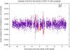 |
Fig. 2 Residuals of the BLS and DST model of CoRoT-1b sampled at 32 s. The central time of the transit chosen has a Julian Date value of 2 454 191.1413 days. The dotted vertical lines indicate the duration of the transit. |
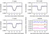 |
Fig. 3 Different models (x2,x4 and BLS) for the light curve of Kepler-22b and comparison of the residuals. |
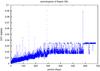 |
Fig. 4 Periodogram of the DST statistic for the light curve of Kepler-22b. This analysis includes 682 days of data from quarters Q0 to Q6 and there are three transit events. |
Relative residuals of the BLS and DST models of the CoRoT-1b and CoRoT id 102763847 targets in parts per million.
3.2. Test case I: the test statistic for a giant planet
It is difficult to compare the result of the test statistics of BLS and DST because they
are defined in different ways and represent different magnitudes. The signal residue (SR)
defined in Kovács et al. (2002) is derived from
expression (5), as has been shown in
Sect. 2. For example, in our particular analysis of
the light curve of CoRoT-1b, the value of the SR, defined as
 in Kovács
et al. (2002), at the ephemeris of the transit has a value of
1.985 18 × 106, whereas it has a value of 1.985 14 × 106
outside the transit, which is a difference of about 22 ppm. However, the statistic used in
BLS is the signal detection efficiency (SDE), built from the SR, which in turn has an
on-transit value of 2.5, and this is the value used to determine the reliability of a
transit candidate. The DST uses expression (14), which is not directly comparable to the SR of BLS. However, in the case of
CoRoT-1b, the value of this estimator on transit is 800 times higher than the value off
transit (3.5 vs. 0.004). If we proceed as in Kovács et al.
(2002) and define an equivalent to the SDE for the DST estimator (see Fig. 5), its value on transit is 6.4, more than doubling the
performance of BLS.
in Kovács
et al. (2002), at the ephemeris of the transit has a value of
1.985 18 × 106, whereas it has a value of 1.985 14 × 106
outside the transit, which is a difference of about 22 ppm. However, the statistic used in
BLS is the signal detection efficiency (SDE), built from the SR, which in turn has an
on-transit value of 2.5, and this is the value used to determine the reliability of a
transit candidate. The DST uses expression (14), which is not directly comparable to the SR of BLS. However, in the case of
CoRoT-1b, the value of this estimator on transit is 800 times higher than the value off
transit (3.5 vs. 0.004). If we proceed as in Kovács et al.
(2002) and define an equivalent to the SDE for the DST estimator (see Fig. 5), its value on transit is 6.4, more than doubling the
performance of BLS.
One of the disadvantages of the SDE statistic is that it includes the points in transit in the calculation of the reference standard deviation used to assess the significance of a signal. This is a known fact already discussed by different authors (see, for example, Kovács et al. 2002; Schwarzenberg-Czerny & Beaulieu 2006; Jenkins et al. 2010b). For example, the WASP survey uses the BLS code for transit detection, but does not use the SDE as statistic to select planetary candidates, but a different statistic with dimensions of χ2 (see Collier Cameron et al. 2006).
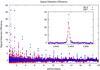 |
Fig. 5 Value of the signal detection efficiency SDE of BLS and DST for the light curve of CoRoT-7b. Detail of the region around the measured orbital period of this planet, indicated with a vertical line (0.853 585 ± 0.000 024 days). |
3.3. Test case II: the test statistic for a terrestrial planet
The difficulty of comparing the performance of different detection algorithms rests in the definition of the test data set and in the optimization of the codes. Simulated data sets have the advantage of handling the impact of the S/N in the detectability of the signals. However, in practice all transit surveys suffer from correlated noise (Pont et al. 2006) that dominates the detectability of dim signals and the rate of false alarms. Therefore we chose for our analysis the measured light curve of CoRoT-7b as test data set. We used standard techniques for filtering stellar variability and instrumental residuals (see below). We did not control how much the red noise affected the detectability of the signal, but we assumed that it would be representative of the typical impact of this kind of perturbation in transit surveys. Lastly, a fair comparison of different techniques requires that the configuration parameters used for the transit search algorithms are optimized with the same rigor. We have done our best to put both algorithms, BLS and DST, in the most similar conditions. Considering the results of the previous section, we assume that the differences in the performance of the analysis of CoRoT-7b that we present are indeed due to the advantages that DST entails over BLS and not due to an improper configuration of the optimizing parameters.
Figure 5 shows the comparison of the SDE defined in the previous subsection for BLS and DST in the analysis of the same light curve of CoRoT-7b. First, DST provides a more robust detection, identifying correctly the right period and many harmonics up to periods of 20 days, and providing a less noisy result than BLS. Second, DST has an SDE of 35 compared to an SDE of only 24 for BLS. This test case shows that DST performs better than BLS also detecting the dim signals of terrestrial planets. Interestingly, the SDE for CoRoT-7b (35) is bigger than the SDE of CoRoT-1b (6.4). There is no reason to be surprised. The SDE is, by definition, a poor posed statistic to characterize the reliability of a signal. The standard deviation of the test statistic is included in the denominator of the SDE. Therefore, a very significant peak, such as that created by a transiting hot Jupiter, will have a significant contribution to the standard deviation of the data, therefore reducing the significance of the SDE (see the discussion in Kovács et al. 2002). If we compare just the value of the test statistic of DST, it has a value of 3.5 in the peak and a background of 0.004 in the case of CoRoT-1b (a ratio of 800) and a value of 0.023 in the peak and a background of 0.0006 in the case of CoRoT-7b (a ratio of 38). As expected, the DST statistic reflects correctly that CoRoT-1b is a more significant detection than CoRoT-7b. This is again a consequence of the definition by Kovács et al. (2002) of the SDE statistic.
4. The transit search paradigm
4.1. The period array
The most common strategy to search for transit-like signals is to perform a blind analysis for an array of test periods. The extremes of the period array are defined according to the expected detectability range: periods shorter than 0.5 days are not expected for planets around solar-like stars because of the vicinity to the host star (as discussed in the introduction). On the other hand, the longest detectable period depends on the length of the observations and the duty cycle. Finally, one has to define the density of periods in the array. Not all authors describe their choices in the literature. Two exceptions are Clarkson et al. (2007), who for the SuperWASP-North survey defined a period range between 0.9 and 5 days with a spacing of 0.002 days for a coarse search and of 0.001 days for a finer search, and Faedi et al. (2011), who used a method equivalent to ours, although in the frequency range. See also the discussion in Jenkins et al. (1996, 2010b).
The light curve is then folded to each value of the period. For each of these periods, the detection algorithm is run for every reasonable combination of transit epoch (from 0 to the end of the folded light curve) and duration of the transit (which can be estimated, for example, from the expected relative sizes of planets around solar-like stars using the expressions in Seager & Mallén-Ornelas 2003). The spacing in the arrays of epochs and durations can be adjusted considering the number of bins in the fold. This method implicitly assumes that there is only one transit per folded light curve.
We propose a method to estimate the best density of the search arrays and an alternative to the blind search described above.
The region in transit T of a folded light curve is defined as the points
in the interval
[x0 − d/2,x0 + d/2] ,
where x0 is the epoch of the transit and d
its duration. If the light curve is not folded, the equivalent definition of the region in
transit is the set of points that verify the condition: ![Mathematical equation: \begin{equation} \label{eq:region_in_transit} x - \mathrm{floor}\left( x/P\right) \cdot P \in \left[x_0-d/2,x_0+d/2\right]. \end{equation}](/articles/aa/full_html/2012/12/aa19337-12/aa19337-12-eq72.png) (16)If we determine the period P
of a transiting planet with an error ΔP and its epoch
x0 with an error Δx0, we can
constrain the position of the Nth transit
xN with an error
ΔxN = Δx0 + N·ΔP.
The position of the Nth transit depends on the length of the observations
I and typically
N ~ I/P.
Therefore, if we aim to constrain the position of the Nth transit with an
uncertainty smaller than a certain value h (for example, comparable to
the sampling rate), the acceptable uncertainty in the period has to fulfill the condition
ΔP < h ∗ P/I.
This condition puts a physical constraint on the desired density of the period array.
(16)If we determine the period P
of a transiting planet with an error ΔP and its epoch
x0 with an error Δx0, we can
constrain the position of the Nth transit
xN with an error
ΔxN = Δx0 + N·ΔP.
The position of the Nth transit depends on the length of the observations
I and typically
N ~ I/P.
Therefore, if we aim to constrain the position of the Nth transit with an
uncertainty smaller than a certain value h (for example, comparable to
the sampling rate), the acceptable uncertainty in the period has to fulfill the condition
ΔP < h ∗ P/I.
This condition puts a physical constraint on the desired density of the period array.
4.2. The region of interest
The region of interest obviously is the transit. The most simple strategy is to search
one transit-like feature per period, neglecting the presence of an occultation or
secondary transit, which is indeed a reasonable assumption for ground-based surveys, and
neglecting the presence of transiting systems of planets. The DST model allows (see
definition 9) to search for
k transit-like features simultaneously without the need of folding the
light curve. The definition of the region in transit
Tk for the kth transit
will be equivalent to (16), substituting
x0 by  , because each transit-like feature will
have a different epoch. One can also use this system to search for secondary transits4 by setting k = 2. Including a second
transit-like feature in the model is not a significant improvement for planet surveys,
because planetary occultations are orders of magnitude lower than primary occultations
(the temperature contrast between the star and the planet is big) and therefore the
improvement of the test statistic will be small. But it can be justified in the case of
eclipsing binaries, where the temperature contrast is comparable and therefore primary and
secondary eclipse have comparable depths. This approach improves the detection and
characterization of eclipsing binaries, which are the main source of contamination in the
search for transiting planets.
, because each transit-like feature will
have a different epoch. One can also use this system to search for secondary transits4 by setting k = 2. Including a second
transit-like feature in the model is not a significant improvement for planet surveys,
because planetary occultations are orders of magnitude lower than primary occultations
(the temperature contrast between the star and the planet is big) and therefore the
improvement of the test statistic will be small. But it can be justified in the case of
eclipsing binaries, where the temperature contrast is comparable and therefore primary and
secondary eclipse have comparable depths. This approach improves the detection and
characterization of eclipsing binaries, which are the main source of contamination in the
search for transiting planets.
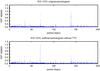 |
Fig. 6 Comparison of the DST detection statistic for KOI 1474 in the original data set (top) and once the transit timing variations were artificially removed (bottom). |
4.3. Transit timing variations
The shape of a transit is markedly affected when folding the light curve of a planet with significant transit timing variation (TTV) assuming a constant period (see, for example, the case of Kepler-9c, Holman et al. 2010). Although our algorithm performs reasonably well when detecting planets or planet candidates with significant TTVs, the current configuration has a limited performance. See, for example, the case of KOI 1474 (Dawson et al. 2012), a transiting Jupiter-sized candidate with a period of ~70 days and TTVs of up to 1h from transit to transit. We analyzed the original Kepler Q0 to Q6 data and calculated the periodogram (see upper part of Fig. 6) and the TTVs. We used the value of the TTVs to artificially shift each transit from the original data to its expected position, if the orbit was exactly periodic, and we recalculated the DST statistic (bottom part of Fig. 6). It now shows a value at the period of the candidate 25% higher. To overcome this effect, we propose another possibility that optimizes the search for planets with significant timing variations. If the observations span an interval I and we are searching for a planet with a period P, we expect k = I/P transits (assuming a full duty cycle). We can define k regions of search and minimize for each region with respect to the epoch of the kth transit, which would be treated independently in the case of large timing variations. Each region k will cover a region of length P since the end of the previous region k − 1. This increases the computational effort, but it provides the best description for this case of scenarios. In the case of Kepler-9c the S/N of the detection was high enough to surmount the degradation of the transit signal. But this might not be the case for small planets close to the noise level. For a given perturber, the timing variations will be stronger for smaller planets (Agol et al. 2005; Holman & Murray 2005; Borkovits et al. 2011). Recently, Carter et al. (2012) mentioned a transit detection algorithm that accounts for variations between consecutive transits, similar to the idea described above, although the algorithm is not described in detail in their paper. We analyzed Kepler public data from quarters Q0 and Q9 with DST and are able to detect both planets with reasonable S/N, although the detection of Kepler-36b is indeed limited by the presence of the TTV (see Fig. 7).
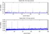 |
Fig. 7 Comparison of the DST detection statistic for the planets of the Kepler-36 system. Kepler-36c (above) with a size of 3.7 Earth radii and a period of 16.2 days produces a clear detection signal in the periodogram. Kepler-36b (below) with a size of 1.5 Earth radii and a period of 13.8 days, which shows significant transit timing variations, produces a distinguishible signal, although limited by the non-periodicity of the transit. |
4.4. False alarms
Every transit detection algorithm based on a test statistic to determine the presence of a transit must use a threshold to distinguish between real and spurious signals. If the probability distribution function of the test statistic is known, it is straightforward to fix the threshold by allowing any desired value of spurious false positives. This procedure is widely discussed in the literature in different contexts (see for example Schwarzenberg-Czerny 1989; Jenkins 2002). However, in practice these limits are not easily applicable. The fundamental assumption that a given statistic follows a particular probability distribution function is that the errors affecting the observations can be treated as random Gaussian variables. Unfortunately, as we show below, this is not the case because most of the remaining residuals, and for sure the most annoying, are always correlated to some degree, invalidating the previous assumption. Therefore, the threshold preventing the appearance of false alarms has to be set accordingly to the level of correlated noise remaining in the light curves, which is method dependent, and not merely to the expected value according to the theoretical behavior of the statistic. All false alarms found in this paper are related to residuals of the stellar activity or instrumental residuals (see below).
5. Future developments
The previous section showed the improvements in the planetary detection performance brought by the better description of the transit shape and the better test statistic for both giant and terrestrial planets. The only drawback of the DST formalism in comparison to BLS is that it involves a slightly heavier computational effort. However, this is only a technical question, not a formal one, and moreover the increase in computational time is not prohibitive. Another advantage of our model is that it keeps the same number of free parameters as BLS, not like the trapezoidal model. The drawback of the computational effort is only an inconvenience and perhaps can be overcome by changing the search strategy. The blind search requires to try, for every trial period, every epoch and duration (or every kth epoch and duration), which is quite expensive and becomes worse with longer exposure intervals, such as those of the Kepler and PLATO surveys. We can overcome this difficulty by changing the paradigm of the search. One can assume that each point of the light curve is the center of a transit-like feature of a given length, therefore defining as many transits as points in the light curve (k = N). Then one can calculate the value of the expressions in (11) for each point and choose which subset of points of the light curve produces a significant change of the test statistic (14). If this subset of points corresponds to a periodic signal, or even multiperiodic in the case of several transiting planets in the system, we have a positive detection. However, one cannot yet find such algorithms in the literature that can select the subset of points that produces a significant change of the test statistic. Searching for these particular algorithms is beyond the scope of this paper, which only aims to present the advantages of the model described in (9), but it will be the subject of future study.
6. Data treatment
We analyzed Q1 data from the Kepler mission. In particular, we use the raw flux column (ap_raw_flux) described in the Kepler data documentation5. We did not use any filter for outliers, relying on the Kepler pipeline for the filtering of cosmic rays. We analyzed each light curve with a Lomb-Scargle periodogram (Scargle 1982) to remove harmonic stellar pulsations. We then applied the stellar variability filter detailed below before using the transit detection algorithm DST to search for the planetary candidates.
6.1. Stellar variability filter
The complex variability pattern of solar-like stars has been studied in the framework of space-based transit surveys such as CoRoT and Kepler (see, for example Aigrain et al. 2009; Gilliland et al. 2011). The stellar variability filter described here is optimized for the removal of the relatively slow changes caused by the evolution of stellar spots modulated by the rotational period of the star. The amplitudes involved in this kind of activity are of a few percent in flux with time-scales of several days. This pattern is regularly observed by space-based telescopes, where targets such as HD 189733 observed by MOST (Croll et al. 2007), CoRoT-2 (Alonso et al. 2008), or HAT-P-11 observed by Kepler (Deming et al. 2011; Sanchis-Ojeda & Winn 2011) are characteristic examples. Other activity patterns such as granulation and related phenomena, which have typical amplitudes in of 0.01% to the ppm range and frequencies of hundreds of μHz, are not treated here.
We assumed that we can separate the incoming flux from the target into a stellar signal
and a planetary transit signal plus some non-correlated residual noise:
 This neglects any contribution from
instrumental features, which in reality will produce correlated residuals. In practice,
the data were pre-treated to remove any previously known instrumental signal6, and any remnant feature will remain in the residuals
(which therefore would not be treatable as random Gaussian variables, as discussed above).
We assumed that the stellar signal Fstar presents some
spot-induced activity signature, which has typical time-scales of days and amplitudes of
few percent; the planetary transit contribution Ftransit is
zero everywhere except during the transits, where it has the characteristic shape of a
transiting planet (see, for example Mandel & Agol
2002). The time-scale of a planetary transit, which is of some hours, is
different from the typical time-scales of the spot induced stellar variability, therefore
we aimed to define an algorithm that can separate both. To build a model of the light
curve that is sensitive only to the long-term stellar variability, we binned the data
adding up to nbin points per bin. This number was chosen for
the purpose of averaging out as much as possible the signatures of transits while the
number of points in the model was dense enough to resolve the stellar variability.
This neglects any contribution from
instrumental features, which in reality will produce correlated residuals. In practice,
the data were pre-treated to remove any previously known instrumental signal6, and any remnant feature will remain in the residuals
(which therefore would not be treatable as random Gaussian variables, as discussed above).
We assumed that the stellar signal Fstar presents some
spot-induced activity signature, which has typical time-scales of days and amplitudes of
few percent; the planetary transit contribution Ftransit is
zero everywhere except during the transits, where it has the characteristic shape of a
transiting planet (see, for example Mandel & Agol
2002). The time-scale of a planetary transit, which is of some hours, is
different from the typical time-scales of the spot induced stellar variability, therefore
we aimed to define an algorithm that can separate both. To build a model of the light
curve that is sensitive only to the long-term stellar variability, we binned the data
adding up to nbin points per bin. This number was chosen for
the purpose of averaging out as much as possible the signatures of transits while the
number of points in the model was dense enough to resolve the stellar variability.
Subsequently we used the Savitzky-Golay approach, which consists in assigning a polynomial model to the original data points that fits the binned data better in a least-squares sense (see Savitzky & Golay 1964; Press et al. 2002). We modeled up to nscale binned data points with a set of Legendre polynomials of degree nLeg. The compromise found between the number of points in the bins nbin, the number of points modeled each iteration nscale and the degree of the polynomials nLeg governs the reaction of the model to the stellar variability and the presence of transits.
A practical procedure to minimize the effect of transits and outliers is to remove the nrem worst points of the fit of the polynomial and recalculate the coefficients of the polynomial with nscale − nrem points. This procedure can be repeated several times (ntimes). Finally, we built Fstar with the values of the polynomials at every time measurement. The values for the different parameters used in this work are summarized in Table 2 and the performance of the filter is shown in two examples named above: CoRoT-2b and HAT-P-11b (Figs. 8 and 9).
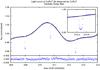 |
Fig. 8 Model of the stellar activity of the CoRoT light curve of CoRoT-2b. The inner box shows the detail of the modeling around one of the transits. The lower box shows the residuals of the modeling. |
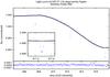 |
Fig. 9 Model of the stellar activity of the Kepler light curve of HAT-P-11b. The inner box shows the detail of the modeling around one of the transits. The lower box shows the residuals of the modeling. |
Configuration parameters of the Savitzky-Golay filter.
The parameters of the filtering method used were optimized for CoRoT data and may not be ideal for the analysis of Kepler data.
However, those parameters were optimized to preserve the shape of transits of short-period planets, such as the ones we expect to detect in the Kepler Q1 data set. They are not optimal for the search of planets with longer periods because they distort the shape of long transit features. For example, in the case of CoRoT-9b (shown in Fig. 10) we needed to use 40 points per bin to preserve the shape of the transit.
Note that the nominal sampling rate of CoRoT is 512 s instead of the nominal sampling rate of 30 min of Kepler, therefore nbin = 20 in the CoRoT sampling rate corresponds approximately to nbin = 5 in the Kepler sampling rate.
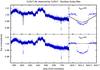 |
Fig. 10 Model of the stellar activity of the light curve of CoRoT-9b with two different values for the configuration of the stellar activity filter. In the top panel, the configuration of the filter is not optimal and the filter tries to remove the transit signal. In the lower panel, the configuration was adapted to preserve the signal of these long transits. |
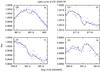 |
Fig. 11 Detail of the light curve of KIC 3340139 observed in the Q0 and Q1 Kepler quarters. The continuous line represents the model of stellar activity together with the transit solution found by DST. Panels b)–d) show residuals of stellar activity that mimic a periodic transit feature. Panel a) shows the expected position of the transit in Q0 data. |
On the other hand, Kepler reaches a higher S/N level than CoRoT and
many stellar activity patterns, which are too small to be important for CoRoT, become
critical for Kepler. This is shown in Fig. 11. The Q1 light curve of KIC 3340139 shows three events approximately separated
by 9.86 days (labeled with the letters b, c, and d in the figure). If they were produced
by a transiting planet around a solar-like star, the size of the planet could be as small
as 1.5 Earth radii. However, those events are not convincing enough: event b is in fact
triggered by only three points ~2σ below the mean. Event c is
probably caused by a residual of the stellar activity on a shorter timescale than the
spot-induced variability. Event d is more similar to a planetary transit event, but the
ingress and egress are not well defined and indeed there are similar features in the light
curve which do not follow any particular periodic pattern. Event a corresponds to Q0 data
and clearly shows no transit-like feature at the expected position of the transit. We
believe that the periodical signal detected by the algorithm in KIC 3340139 is an artifact
caused by residuals of the stellar activity that wer not properly handled by the filter
because of their short typical timescales, comparable to the duration of a planetary
transit. An important indication against the planetary origin of the events is that if the
configuration of the stellar activity filter is changed, for example making
nbin = 8, no periodical signal is detected in the light
curve any more. Any detection that depends so strongly on the filtering method is not
reliable. From another standpoint, the activity level displayed by KIC 3340139 is not
unusual. The light curve of the LRa01 run from CoRoT 102584409 (a star with a similar
magnitude to KIC 3340139, r′ = 11.44 mag
and Kp = 11.46 mag respectively) shows a similar activity
pattern (see Fig. 12), but CoRoT is not sensitive
to the small amplitude, short timescale patterns such as event c in Fig. 11. Figure 13
compares the noise level of these particular CoRoT and Kepler targets
following the procedure described by Pont et al.
(2006), which separates the contributions of the non-correlated (also known as
white) noise, which evolves as 1/ , being n the number of
binned flux values, and the correlated (also known as red) noise. The filter applied here
was optimized for CoRoT data and is insensitive to the patterns displayed by KIC 3340139.
We consider optimizing the algorithm filtering the stellar activity for small
Kepler transits in future work.
, being n the number of
binned flux values, and the correlated (also known as red) noise. The filter applied here
was optimized for CoRoT data and is insensitive to the patterns displayed by KIC 3340139.
We consider optimizing the algorithm filtering the stellar activity for small
Kepler transits in future work.
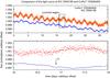 |
Fig. 12 Comparison of the light curves of KIC 3340139 and CoRoT 102584409, which show similar activity levels. The position of event c from Fig. 11 is marked with an arrow in the lower panel. |
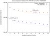 |
Fig. 13 Analysis of the noise level of the light curves of KIC 3340139 and CoRoT 102584409.
The typical noise level within 1h in the CoRoT light curve is equivalent to the
depth of a transit of a 1.6 RE planet around a
solar-like star. The typical noise level for the Kepler light curve
in 1 h is equivalent to the depth of a transit of a
0.87 RE planet. The dotted line shows the
1/ |

This limitation of the stellar activity filtering created a considerable number of false alarms in this data set compared to what is usual when analyzing CoRoT data (more than 100), which were removed by running the filtering method again with slightly different parameters and by comparing the results of the transit detection analysis in the new filtered data. Any detection that depended on the filtering method was rejected as a false alarm. As these are dependent on the stellar filtering method applied and not on the detection method, they are not listed in this paper.
7. Results
As discussed before, one of the main conclusion of the studies carried out by the CoRoT community when testing different transit detection algorithms was that both detections and false alarms were method dependent (Moutou et al. 2005, 2007). In our analysis of the Q1 data set we found that both statements are still true when comparing our results to those from the Kepler community.
7.1. The yield of detections
We found 43 planetary candidates analyzing 33 days of data that went unnoticed to B11b, among them 8 multiple transiting systems. Most of them were discovered later by Batalha et al. (2012), who analyzed 480 days of data, but not all of them. There are still 15 planetary candidates, among them 3 multiple transiting systems, not discovered and published by the Kepler team7. The advantage of having an algorithm that can detect new candidates in a significantly reduced data set is twofold. On the one hand, the fewer transits needed to find a planet, the earlier can the follow-up begin, which is a critical point in the design of transit surveys because the resources are limited. On the other hand, the most interesting planets, such as terrestrial planets in the habitable zone of solar-like stars, have long periods, typically comparable to years, and will typically have few transit events. If we compare the distribution of our new candidates with those from B11b, we can see that the bulk of our detections has periods between five and ten days (see Fig. 14), which corresponds to candidates having six to three transit events in our data set.
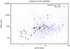 |
Fig. 14 Comparison of the depth and the period of the planetary candidates found in this work compared to those of B11b. |
Table 3 contains the ephemeris of the new planetary candidates not found by B11b, nor found as eclipsing binaries by Prša et al. (2011) or Slawson et al. (2011). Some of them were later found by Batalha et al. (2012); when this is the case, the KOI number assigned by the Kepler team is shown to identify them. These candidates were ranked according to the CoRoT rules (see Carpano et al. 2009; Cabrera et al. 2009). Note the presence of several planetary candidates similar to CoRoT-7b (Léger et al. 2009; Queloz et al. 2009) and Kepler-10b (Batalha et al. 2011) in period and depth (they are marked with the label C7b-like). To detect the candidates we only used data from Q1, but to characterize the candidates and calculate the ephemeris we used public Kepler data from other runs to improve the ephemeris and confirm the detection.
Table 4 contains the ephemeris of our false positives: detections ranked by the CoRoT rules that turned out to be background eclipsing binaries identified by the study of the centroid motion (Batalha et al. 2010). The responsible contaminating eclipsing binary or its position within the mask is indicated in the table.
Finally, Table 5 contains the ephemeris of the false alarms found in our analysis of the Q1 data, which are discussed below in Sect. 7.3.
7.2. Kepler candidates not detected by our pipeline
We studied the candidates found in B11b that were not found by our analysis and discuss in the following sections possible reasons for these non-detections. Both data sets are not immediately comparable, because B11b corresponds to four times more data than the analyzed here, and therefore we do not expect to find all. Still, we can learn about the performance of our algorithm and about the Kepler data set from these non-detections, as we detail below.
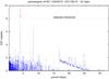 |
Fig. 15 Periodogram of KIC 10454313 showing the position of the peak corresponding to the planet candidate KOI 532.01, marked with an arrow. The height of the peak is 7.9, directly below the detection threshold (see discussion in text). |
Parameters from the planetary candidates.
Parameters from the false positives.
Parameters from the false alarms.
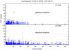 |
Fig. 16 Periodogram of KIC 9119458. The upper part corresponds to the analysis of the data set Q1 and the peak of the candidate 525.01 is marked with an arrow. Its height is 5.4, well below the detection threshold. The lower part corresponds to the analysis of the data set Q2, where the height of the peak is 12.8 (see discussion in text). |
7.2.1. Candidates below the detection threshold
In several cases, we found B11bKepler candidates below our detection threshold. The threshold was optimized according to the CoRoT experience and was fixed at a S/N of 8 between the peak and the background. Several candidates, which could be clearly detected in the light-curves, produced periodograms with peaks immediately below the fixed threshold (see, for example, the case of the candidate KOI 532.01 from B11b shown in Fig. 15). In the absence of red noise, this detection threshold can be fixed for a particular detection algorithm by making the probability of detecting a false alarm as low as needed (see, for example, Jenkins et al. 2002). However, in practice the presence of correlated residuals in the light curves distorts the expected distribution of false alarms and it is advisable to use a more conservative value of the threshold. An illustrating case is shown in Fig. 16, where the Q1 data set alone, which includes three transit events, barely suffices to distinguish between the genuine peak from the candidate KOI 525.01 from B11b. For comparison, in the lower part of Fig. 16 the analysis of the data set Q2, which contains seven transit events, is shown. In this data set the peak clearly rises above the fixed threshold. Considering the level of the correlated residuals in the Q1 data set, the threshold applied in the analysis presented in this paper seems to be too conservative.
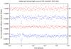 |
Fig. 17 Comparison of the light curves of the target KIC 6422367 folded at the period and phase of the planetary candidate KOI 559.01. The signal of the candidate is not visible in quarters Q1, Q3, and Q4 (not shown). See discussion in text. |
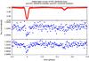 |
Fig. 18 Comparison of the light curves of the targets KIC 2830919 and KIC 3325239 folded at the ephemeris of the eclipsing binary KIC 3836439. See discussion in text. |
7.2.2. Instrumental effects
Among the candidates not found in our analysis there is a very particular case that is worth mentioning. The planet candidate from B11b KOI 559.01 (KIC 6422367) was not found in the Q1 data set. We looked for the candidate in the Q2 data set and we were able to find it, but with a significantly different depth, 700 ± 70 ppm, than the one reported in the original paper (214 ppm). We pursued our analysis on this particular candidate by analyzing the latest data sets released by the Kepler team (see Fig. 17) and realized that the candidate was only present in the Q2 and Q6 data sets, not in Q1, Q3 and Q4 (there is no Q5 data for this target because of the failure of module 3). We note that from Q2 to Q6 the satellite performs a full revolution maneuver. This behavior is typical of a contamination from a background eclipsing binary, which only pollutes the PSF of the candidate in particular orientations of the CCD. We searched for an eclipsing binary that could be the origin of this contamination in the field of view of Kepler and found that KIC 6422367 has the same period and roughly the same phase as the candidate. The periods of the candidate and the binary are 4.331 39 (5) days and 4.331 398(1) days respectively; the epochs are (HJD-2 451 545.0) 121.722 (4) and 121.732 21 (7). The main counterargument of this explanation is that this eclipsing binary is 1.8° away from the candidate (for example, during Q2, the eclipsing binary was observed in module 11 in channel 34, whereas the planetary candidate was observed in the same module, but in channel 36). The probability that two independent targets have the same period and phase is extremely low. On the other hand, this phenomenon could have an instrumental origin. In support of this hypothesis, we have found two more examples of this behavior. The targets KIC 2830919 and KIC 3325239 show the same ephemeris as the eclipsing binary KIC 3836439 (see Fig. 18). The first target is at 1.4° of the binary and the second at 0.8°. KIC 3325239 clearly shows the alternates of appearance in quarters Q1 and Q5, while it disappears in quarters Q2, Q3, Q4 and Q6 (see Fig. 19). In space-based surveys, the contamination of neighbor targets by a bright eclipsing binary, such as the contamination of KIC 9641031 of the targets KIC 9640985, KIC 9641008, KIC 9641041, and the planet candidate KOI 712.01 (KIC 9640976, which is then a false alarm despite of being ranked as a planet candidate in B11b, see Fig. 20), is well known (see, for example, Deeg et al. 2009; Batalha et al. 2010), but to our knowledge the type of contamination presented here has not been documented before. Recently, Batalha et al. (2012) discussed the possibility that scattered light from bright eclipsing binaries contaminates the masks of neighboring targets. However, these authors referred to targets within 20′′ of the binary, whereas the contamination that we have observed originates in targets more than 1 arc degree away. The origin of this contamination deserves a more detailed study, which is beyond the scope of this paper. The reason for this behavior might be an effect named video cross-talk (Van Cleve & Caldwell 2009; Jenkins, priv. comm.).
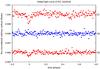 |
Fig. 19 Comparison of the light curves of the target KIC 3325239 folded at the period and phase of the eclipsing binary KIC 3836439. From top to bottom the data of quarters Q1, Q2, and Q5 are shown. The signal is only visible in quarters Q1 and Q5. See discussion in text. |
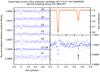 |
Fig. 20 Comparison of the light curves of the planetary candidate KOI 712.01 (KIC 9640976) and the eclipsing binary KIC 9641031. The left side of the figure shows the data of KOI 712.01 from the different quarters. The transit events are not seen in Q1, and the transit depth is not constant in quarters Q2 to Q6. The top part of the right side shows the light curve of the eclipsing binary and the lower part the data from quarters Q1 to Q6 of 712.01 folded at the ephemeris of the eclipsing binary. The secondary eclipse is visible in this data set (marked with an arrow in the figure). |
7.2.3. False positives from the Kepler pipeline
In addition to the cases of KOI 559.01 and KOI 712.01 described above, there are other clear false alarms unnoticed among the planetary candidates in B11b.
-
KOI 774 shows aclear eccentric secondary eclipse onthe 3 × 10⁻⁴ level (300 ppm), incompatible with the occultation of a planetary companion (see Coughlin & López-Morales 2012). This candidate has been classified as an eclipsing binary by Slawson et al. (2011).
-
KOI 823 shows out-of-transit variations compatible with a massive companion and a secondary eclipse on the 7 × 10⁻⁴ level, incompatible with the occultation of a planetary companion. This candidate was also classified as a potential false positive by Demory & Seager (2011).
-
KOI 876 shows a secondary eclipse on the 7 × 10⁻⁴ level, incompatible with the occultation of a planetary companion. This candidate was also classified as a false positive by Demory & Seager (2011).
-
KOI 960 shows an eccentric secondary eclipse on the 5 × 10⁻⁴ level, incompatible with the occultation of a planetary companion. This candidate was also classified as a potential false positive by Demory & Seager (2011).
-
KOI 1285 shows a secondary eclipse on the 3 × 10⁻⁴ level, incompatible with the occultation of a planetary companion. Additionally, it shows strong eclipse timing variations, indicating the presence of either stellar interaction or additional companions in the system. This candidate has been classified as an eclipsing binary by Slawson et al. (2011) and also classified as a potential false positive by Demory & Seager (2011).
-
KOI 1401 displays the typical out-of-eclipse behavior of an eclipsing binary and has been classified as such by Slawson et al. (2011).
-
KOI 1448 is an active star, the light curve shows a secondary eclipse on the 8 × 10⁻⁴ level, incompatible with the occultation of a planetary companion, and has been classified as an eclipsing binary by Slawson et al. (2011) and also classified as a false positive by Demory & Seager (2011).
-
KOI 1452 is another active star with a secondary eclipse on the 1 × 10⁻³ level, incompatible with the occultation of a planetary companion, and has been classified as an eclipsing binary by Slawson et al. (2011).
-
KOI 1459 is an eclipsing binary with a real period of 1.38 days, twice that found by B11b and Slawson et al. (2011). The depths of the primary and secondary eclipses are 0.45 ± 0.01 and 0.36 ± 0.01.
-
KOI 1541 shows a secondary eclipse on the 1 × 10⁻³ level, incompatible with the occultation of a planetary companion, and has been classified as an eclipsing binary by Slawson et al. (2011).
-
KOI 1543 shows a secondary eclipse on the 1 × 10⁻³ level, incompatible with the occultation of a planetary companion. It was classified as an eclipsing binary with the wrong period of 7.92 days by Prša et al. (2011), the real period is half that or 3.96 days, but it is not in the list of binaries by Slawson et al. (2011) although it was classified as a false positive by Demory & Seager (2011).
-
KOI 1546 shows out-of-transit variations compatible with an eclipsing binary and was classified as such by Prša et al. (2011), but not by Slawson et al. (2011).
For completion, we add that the candidates KOI 4, KOI 51, KOI 131, KOI 135, KOI 138, KOI 201, KOI 206, KOI 211, KOI 225, KOI 256, KOI 261, KOI 340, KOI 687, KOI 741, KOI 822, KOI 913, KOI 976, KOI 1187, KOI 1020, KOI 1032, KOI 1227, and KOI 1385 have also been classified either by Prša et al. (2011) or by Slawson et al. (2011) as eclipsing binaries, and considering their light curves, they probably are. They all still appear as valid planetary candidates in the list of Batalha et al. (2012), because the vetting of the first 1600 KOIs has not been reprocessed with the improved method described in that paper which has been used for the most recent release of KOIs8. They represent a small fraction of the total number of candidates, but they are still readily identifiable by a careful analysis of the light curve. The careful tests applied by the Kepler pipeline could not remove these easily identificable false positives. One may wonder how many of the remaining candidates with lower S/N, in which region those tests are less sensitive, will turn out to be also false positives. Authors should be extremely careful when interpreting the statistical analysis based on candidates without radial velocity confirmation or candidates that have not been properly validated (Torres et al. 2011).
7.2.4. Other reasons
In 14 cases either the stellar variability filter failed to remove the stellar signal without damaging the transit signal (for example, in the case of KOI 242, with a transit duration of almost 6 h, see Fig. 21) or some residual outliers prevented the candidate detection. As we mentioned above, we relied on the cosmic ray filtering of the Kepler pipeline. In some cases, remaining outliers in the light curve prevented the detection of candidates such as KOI 234 (see Fig. 22) with our algorithm, but these cases represent a minority of the non-detections. The stellar variability filtering is performing well, allowing the detection of most of the expected Kepler candidates, although it could be improved to enhance the detection of weaker signals of yet undetected transit candidates.
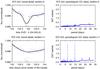 |
Fig. 21 Light curve of KOI 242 filtered with the original configuration used for the analysis in this paper (top) and with an alternative configuration (bottom) that prevents the filtering of long transits. |
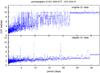 |
Fig. 22 Above: periodogram of KOI 234 (KIC 8491277) in the original Q1 data set. Below, the same periodogram after applying a 4σ clipping to the light curve. The candidate, which could not be distinguished from the noise in the original data set, is clearly detected in the filtered data set. |
7.3. False alarms from our pipeline
The false alarms in Table 5 were identified because they could be detected in the Q1 data set, but not in subsequent runs. We present as an illustrating example the case of KIC 11350341 (see Fig. 23). The periodogram of the Q1 data set has a distinct peak at the period of 9.3 days caused by thre transit events visible in the raw light curve. However, subsequent observations during the quarters Q2 to Q6 do not show the presence of this periodic signal. We do not find any nearby contaminating eclipsing binary that could be responsible of the signal. However, there are some nearby variable stars that contaminate the mask. Possibly the stellar activity filter is not completely removing their contribution, and therefore the residuals produce the spurious detection. We think that the Q1 data suffers from more contamination from neighboring sources than subsequent runs, which could explain why false alarms are only present in the Q1 data. One of the reasons for this additional contamination would be the presence of a variable star among the guiding stars in Q1 (see the discussion in Caldwell et al. 2010; Haas et al. 2010; Jenkins et al. 2010a). Another possible reason are instrumental effects such as those described above in the case of KOI 559.01.
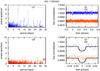 |
Fig. 23 Left: periodograms of the Q1 (top) and Q2 (bottom) data sets of the target KIC 11350341. Only the Q1 data show a periodic signal. Right: filtered and folded light curve of KIC 11350341. Q1 data distinctly show a transiting signal, which cannot be recovered in Q2 data. |
8. Summary
We have described a new algorithm for transit detection using an analytic model for the shape of a transit (Sect. 2). We have compared in Sect. 3 the performance of the new transit detection technique, DST, with that of a widely used technique, the BLS algorithm, and showed that our algorithm performs better. We analyzed two representative test cases and concluded that DST produces a better signal detection efficiency than BLS due to the improved description of the transit signal and to the improved definition of the test statistic in all relevant cases for transit surveys: terrestrial planets, giant planets, and eclipsing binaries. We discussed the advantages and the flexibility of this algorithm in defining the region in transit (Sect. 4), with their implications for the search for planets that experience significant transit timing variations (Sect. 4.3) and transiting multiple planet systems (Sect. 5). We intend to develop methods to make the computational effort required by this algorithm more effective in the future by changing the paradigm of the blind transit searches, as described in Sect. 5.
We applied our algorithm and a set of tools to filter the stellar activity, which was designed for the CoRoT search of transiting planets, to the publicly released Q1 Kepler data. As a result of this analysis, some adjustments were made to improve the performance of the stellar activity filtering. We report 15 planetary candidates, not reported previously in the literature, based on our analysis of 33 days of Kepler data. We discussed the impact of instrumental and stellar activity residuals in the data on the detection of planetary candidates. Our study shows that the analysis of space mission data advocates the use of complementary detrending and transit detection tools for future space-based transit surveys such as PLATO (Catala 2009).
CoRoT public data is available thorough the CoRoT Data Archive hosted by IAS: http://idoc-corot.ias.u-psud.fr
CoRoT-1b was observed at 512 s and 32 s sampling rate during the run IRa01, described in Carpano et al. (2009), where it got the win_id IRa01_E2_1126. The eclipsing binary with CoRoT id 102763847 was observed at 32 s sampling rate during the run IRa01, where it got the win_id IRa01_E1_1158, and at 512 s sampling rate during the run LRa01 (Carone et al. 2012), where it got the win_id LRa01_E2_0588.
The code is available on request to the author.
The computational effort can be reduced by assuming circular orbits and fixing
 but this assumption is only reasonable for
short periods.
but this assumption is only reasonable for
short periods.
In the latest released version of Kepler data, the raw flux column is called sap_flux. See http://keplergo.arc.nasa.gov/Documentation.shtml
For example, in the CoRoT context, any periodical variation at the orbital period of the satellite.
While our paper was in the revision process, Ofir & Dreizler (2012) published 84 new transiting signals in the Kepler data.
While our paper was in the revision process, Ofir & Dreizler (2012) provided arguments to reclassify some additional KOIs as eclipsing binaries.
Acknowledgments
We would like to thank Jon Jenkins and our anonymous referee for their insightful reading of our manuscript and their detailed comments, which improved our manuscript. Kepler data presented in this paper were obtained from the Multimission Archive at the Space Telescope Science Institute (MAST). STScI is operated by the Association of Universities for Research in Astronomy, Inc., under NASA contract NAS5-26555. Support for MAST for non-HST data is provided by the NASA Office of Space Science via grant NNX09AF08G and by other grants and contracts The CoRoT space mission, launched on December 27, 2006, was developed and is operated by CNES, with contributions from Austria, Belgium, Brazil, ESA, Germany and Spain. This research has made use of NASA’s Astrophysics Data System.
References
- Agol, E., Steffen, J., Sari, R., & Clarkson, W. 2005, MNRAS, 359, 567 [NASA ADS] [CrossRef] [Google Scholar]
- Aigrain, S., & Favata, F. 2002, A&A, 395, 625 [NASA ADS] [CrossRef] [EDP Sciences] [Google Scholar]
- Aigrain, S., Pont, F., Fressin, F., et al. 2009, A&A, 506, 425 [NASA ADS] [CrossRef] [EDP Sciences] [Google Scholar]
- Alonso, R., Auvergne, M., Baglin, A., et al. 2008, A&A, 482, L21 [NASA ADS] [CrossRef] [EDP Sciences] [Google Scholar]
- Baglin, A., Auvergne, M., Boisnard, L., et al. 2006, in 36th COSPAR Scientific Assembly, 3749 [Google Scholar]
- Barge, P., Baglin, A., Auvergne, M., et al. 2008, A&A, 482, L17 [NASA ADS] [CrossRef] [EDP Sciences] [Google Scholar]
- Batalha, N. M., Rowe, J. F., Gilliland, R. L., et al. 2010, ApJ, 713, L103 [NASA ADS] [CrossRef] [Google Scholar]
- Batalha, N. M., Borucki, W. J., Bryson, S. T., et al. 2011, ApJ, 729, 27 [NASA ADS] [CrossRef] [Google Scholar]
- Batalha, N. M., Rowe, J. F., Bryson, S. T., et al. 2012, ApJS, submitted [arXiv:1202.5852] [Google Scholar]
- Bonomo, A. S., & Lanza, A. F. 2008, A&A, 482, 341 [NASA ADS] [CrossRef] [EDP Sciences] [Google Scholar]
- Bordé, P., Fressin, F., Ollivier, M., Léger, A., & Rouan, D. 2007, in Transiting Extrapolar Planets Workshop, eds. C. Afonso, D. Weldrake, & T. Henning, ASP Conf. Ser., 366, 145 [Google Scholar]
- Borkovits, T., Csizmadia, S., Forgács-Dajka, E., & Hegedüs, T. 2011, A&A, 528, A53 [NASA ADS] [CrossRef] [EDP Sciences] [Google Scholar]
- Borucki, W. J., Koch, D., Basri, G., et al. 2010, Science, 327, 977 [NASA ADS] [CrossRef] [PubMed] [Google Scholar]
- Borucki, W. J., Koch, D. G., Basri, G., et al. 2011a, ApJ, 728, 117 [NASA ADS] [CrossRef] [Google Scholar]
- Borucki, W. J., Koch, D. G., Basri, G., et al. 2011b, ApJ, 736, 19 [NASA ADS] [CrossRef] [Google Scholar]
- Borucki, W. J., Koch, D. G., Batalha, N., et al. 2012, ApJ, 745, 120 [NASA ADS] [CrossRef] [Google Scholar]
- Cabrera, J., Fridlund, M., Ollivier, M., et al. 2009, A&A, 506, 501 [NASA ADS] [CrossRef] [EDP Sciences] [Google Scholar]
- Caldwell, D. A., Kolodziejczak, J. J., Van Cleve, J. E., et al. 2010, ApJ, 713, L92 [NASA ADS] [CrossRef] [Google Scholar]
- Carone, L., Gandolfi, D., Cabrera, J., et al. 2012, A&A, 538, A112 [NASA ADS] [CrossRef] [EDP Sciences] [Google Scholar]
- Carpano, S., & Fridlund, M. 2008, A&A, 485, 607 [NASA ADS] [CrossRef] [EDP Sciences] [Google Scholar]
- Carpano, S., Cabrera, J., Alonso, R., et al. 2009, A&A, 506, 491 [NASA ADS] [CrossRef] [EDP Sciences] [Google Scholar]
- Carter, J. A., Agol, E., Chaplin, W. J., et al. 2012, Science, 337, 556 [NASA ADS] [CrossRef] [PubMed] [Google Scholar]
- Catala, C. 2009, Exp. Astron., 23, 329 [NASA ADS] [CrossRef] [Google Scholar]
- Cavarroc, C., Moutou, C., Gandolfi, D., et al. 2012, Ap&SS, 337, 511 [NASA ADS] [CrossRef] [Google Scholar]
- Charbonneau, D., Berta, Z. K., Irwin, J., et al. 2009, Nature, 462, 891 [NASA ADS] [CrossRef] [PubMed] [Google Scholar]
- Clarkson, W. I., Enoch, B., Haswell, C. A., et al. 2007, MNRAS, 381, 851 [NASA ADS] [CrossRef] [Google Scholar]
- Collier Cameron, A., Pollacco, D., Street, R. A., et al. 2006, MNRAS, 373, 799 [NASA ADS] [CrossRef] [Google Scholar]
- Coughlin, J. L., & López-Morales, M. 2012, AJ, 143, 39 [NASA ADS] [CrossRef] [Google Scholar]
- Croll, B., Matthews, J. M., Rowe, J. F., et al. 2007, ApJ, 671, 2129 [NASA ADS] [CrossRef] [Google Scholar]
- Dawson, R. I., Johnson, J. A., Morton, T. D., et al. 2012, ApJ, in press [arXiv:1206.5579] [Google Scholar]
- Deeg, H. J., Gillon, M., Shporer, A., et al. 2009, A&A, 506, 343 [NASA ADS] [CrossRef] [EDP Sciences] [Google Scholar]
- Deeg, H. J., Moutou, C., Erikson, A., et al. 2010, Nature, 464, 384 [NASA ADS] [CrossRef] [PubMed] [Google Scholar]
- Defaÿ, C., Deleuil, M., & Barge, P. 2001, A&A, 365, 330 [NASA ADS] [CrossRef] [EDP Sciences] [Google Scholar]
- Deming, D., Sada, P. V., Jackson, B., et al. 2011, ApJ, 740, 33 [NASA ADS] [CrossRef] [Google Scholar]
- Demory, B.-O., & Seager, S. 2011, ApJS, 197, 12 [NASA ADS] [CrossRef] [Google Scholar]
- Erikson, A., Santerne, A., Renner, S., et al. 2012, A&A, 539, A14 [NASA ADS] [CrossRef] [EDP Sciences] [Google Scholar]
- Faedi, F., West, R. G., Burleigh, M. R., Goad, M. R., & Hebb, L. 2011, MNRAS, 410, 899 [NASA ADS] [CrossRef] [Google Scholar]
- Gilliland, R. L., Chaplin, W. J., Dunham, E. W., et al. 2011, ApJS, 197, 6 [NASA ADS] [CrossRef] [Google Scholar]
- Grziwa, S., Pätzold, M., & Carone, L. 2012, MNRAS, 420, 1045 [NASA ADS] [CrossRef] [Google Scholar]
- Haas, M. R., Batalha, N. M., Bryson, S. T., et al. 2010, ApJ, 713, L115 [NASA ADS] [CrossRef] [Google Scholar]
- Hebb, L., Collier-Cameron, A., Triaud, A. H. M. J., et al. 2010, ApJ, 708, 224 [NASA ADS] [CrossRef] [Google Scholar]
- Hellier, C., Anderson, D. R., Collier Cameron, A., et al. 2009, Nature, 460, 1098 [NASA ADS] [CrossRef] [Google Scholar]
- Hellier, C., Anderson, D. R., Collier Cameron, A., et al. 2011, A&A, 535, L7 [NASA ADS] [CrossRef] [EDP Sciences] [Google Scholar]
- Holman, M. J., & Murray, N. W. 2005, Science, 307, 1288 [NASA ADS] [CrossRef] [PubMed] [Google Scholar]
- Holman, M. J., Fabrycky, D. C., Ragozzine, D., et al. 2010, Science, 330, 51 [NASA ADS] [CrossRef] [PubMed] [Google Scholar]
- Jenkins, J. M. 2002, ApJ, 575, 493 [NASA ADS] [CrossRef] [Google Scholar]
- Jenkins, J. M., Doyle, L. R., & Cullers, D. K. 1996, Icarus, 119, 244 [NASA ADS] [CrossRef] [Google Scholar]
- Jenkins, J. M., Caldwell, D. A., & Borucki, W. J. 2002, ApJ, 564, 495 [NASA ADS] [CrossRef] [Google Scholar]
- Jenkins, J. M., Caldwell, D. A., Chandrasekaran, H., et al. 2010a, ApJ, 713, L120 [NASA ADS] [CrossRef] [Google Scholar]
- Jenkins, J. M., Chandrasekaran, H., McCauliff, S. D., et al. 2010b, in SPIE Conf. Ser., 7740 [Google Scholar]
- Kovács, G., Zucker, S., & Mazeh, T. 2002, A&A, 391, 369 [NASA ADS] [CrossRef] [EDP Sciences] [Google Scholar]
- Léger, A., Rouan, D., Schneider, J., et al. 2009, A&A, 506, 287 [NASA ADS] [CrossRef] [EDP Sciences] [MathSciNet] [Google Scholar]
- Mandel, K., & Agol, E. 2002, ApJ, 580, L171 [NASA ADS] [CrossRef] [Google Scholar]
- Moutou, C., Pont, F., Barge, P., et al. 2005, A&A, 437, 355 [NASA ADS] [CrossRef] [EDP Sciences] [Google Scholar]
- Moutou, C., Aigrain, S., Almenara, J., et al. 2007, in Transiting Extrapolar Planets Workshop, eds. C. Afonso, D. Weldrake, & T. Henning, ASP Conf. Ser., 366, 127 [Google Scholar]
- Ofir, A. 2008, MNRAS, 387, 1597 [NASA ADS] [CrossRef] [Google Scholar]
- Ofir, A., & Dreizler, S. 2012, A&A, submitted [arXiv:1206.5347] [Google Scholar]
- Pont, F., Zucker, S., & Queloz, D. 2006, MNRAS, 373, 231 [NASA ADS] [CrossRef] [Google Scholar]
- Press, W. H., Teukolsky, S. A., Vetterling, W. T., & Flannery, B. P. 2002, Numerical Recipes in C++, 2nd edn. (Cambridge University Press) [Google Scholar]
- Protopapas, P., Jimenez, R., & Alcock, C. 2005, MNRAS, 362, 460 [NASA ADS] [CrossRef] [Google Scholar]
- Prša, A., Batalha, N., Slawson, R. W., et al. 2011, AJ, 141, 83 [NASA ADS] [CrossRef] [Google Scholar]
- Queloz, D., Bouchy, F., Moutou, C., et al. 2009, A&A, 506, 303 [NASA ADS] [CrossRef] [EDP Sciences] [Google Scholar]
- Régulo, C., Almenara, J. M., Alonso, R., Deeg, H., & Roca Cortés, T. 2007, A&A, 467, 1345 [NASA ADS] [CrossRef] [EDP Sciences] [Google Scholar]
- Renner, S., Rauer, H., Erikson, A., et al. 2008, A&A, 492, 617 [NASA ADS] [CrossRef] [EDP Sciences] [Google Scholar]
- Sanchis-Ojeda, R., & Winn, J. N. 2011, ApJ, 743, 61 [NASA ADS] [CrossRef] [Google Scholar]
- Savitzky, A., & Golay, M. J. E. 1964, Anal. Chem., 36, 1627 [NASA ADS] [CrossRef] [Google Scholar]
- Scargle, J. D. 1982, ApJ, 263, 835 [NASA ADS] [CrossRef] [Google Scholar]
- Schwarzenberg-Czerny, A. 1989, MNRAS, 241, 153 [NASA ADS] [CrossRef] [Google Scholar]
- Schwarzenberg-Czerny, A. 1998, Baltic Astron., 7, 43 [NASA ADS] [Google Scholar]
- Schwarzenberg-Czerny, A., & Beaulieu, J. 2006, MNRAS, 365, 165 [NASA ADS] [CrossRef] [Google Scholar]
- Seager, S., & Mallén-Ornelas, G. 2003, ApJ, 585, 1038 [NASA ADS] [CrossRef] [Google Scholar]
- Slawson, R. W., Prša, A., Welsh, W. F., et al. 2011, AJ, 142, 160 [NASA ADS] [CrossRef] [Google Scholar]
- Tingley, B. 2003a, A&A, 403, 329 [NASA ADS] [CrossRef] [EDP Sciences] [Google Scholar]
- Tingley, B. 2003b, A&A, 408, L5 [NASA ADS] [CrossRef] [EDP Sciences] [Google Scholar]
- Torres, G., Fressin, F., Batalha, N. M., et al. 2011, ApJ, 727, 24 [NASA ADS] [CrossRef] [Google Scholar]
- Van Cleve, J. E., & Caldwell, D. A. 2009, Kepler Instrument Handbook (KSCI-19033) (NASA) [Google Scholar]
- Winn, J. N., Matthews, J. M., Dawson, R. I., et al. 2011, ApJ, 737, L18 [NASA ADS] [CrossRef] [Google Scholar]
All Tables
Relative residuals of the BLS and DST models of the CoRoT-1b and CoRoT id 102763847 targets in parts per million.
All Figures
|
Fig. 1 Residuals of the BLS and DST model of CoRoT-1b sampled at 512 s. The central time of the transit chosen has a Julian Date value of 2 454 142.8547 days. The dotted vertical lines indicate the duration of the transit. |
| In the text | |
|
Fig. 2 Residuals of the BLS and DST model of CoRoT-1b sampled at 32 s. The central time of the transit chosen has a Julian Date value of 2 454 191.1413 days. The dotted vertical lines indicate the duration of the transit. |
| In the text | |
|
Fig. 3 Different models (x2,x4 and BLS) for the light curve of Kepler-22b and comparison of the residuals. |
| In the text | |
|
Fig. 4 Periodogram of the DST statistic for the light curve of Kepler-22b. This analysis includes 682 days of data from quarters Q0 to Q6 and there are three transit events. |
| In the text | |
|
Fig. 5 Value of the signal detection efficiency SDE of BLS and DST for the light curve of CoRoT-7b. Detail of the region around the measured orbital period of this planet, indicated with a vertical line (0.853 585 ± 0.000 024 days). |
| In the text | |
|
Fig. 6 Comparison of the DST detection statistic for KOI 1474 in the original data set (top) and once the transit timing variations were artificially removed (bottom). |
| In the text | |
|
Fig. 7 Comparison of the DST detection statistic for the planets of the Kepler-36 system. Kepler-36c (above) with a size of 3.7 Earth radii and a period of 16.2 days produces a clear detection signal in the periodogram. Kepler-36b (below) with a size of 1.5 Earth radii and a period of 13.8 days, which shows significant transit timing variations, produces a distinguishible signal, although limited by the non-periodicity of the transit. |
| In the text | |
|
Fig. 8 Model of the stellar activity of the CoRoT light curve of CoRoT-2b. The inner box shows the detail of the modeling around one of the transits. The lower box shows the residuals of the modeling. |
| In the text | |
|
Fig. 9 Model of the stellar activity of the Kepler light curve of HAT-P-11b. The inner box shows the detail of the modeling around one of the transits. The lower box shows the residuals of the modeling. |
| In the text | |
|
Fig. 10 Model of the stellar activity of the light curve of CoRoT-9b with two different values for the configuration of the stellar activity filter. In the top panel, the configuration of the filter is not optimal and the filter tries to remove the transit signal. In the lower panel, the configuration was adapted to preserve the signal of these long transits. |
| In the text | |
|
Fig. 11 Detail of the light curve of KIC 3340139 observed in the Q0 and Q1 Kepler quarters. The continuous line represents the model of stellar activity together with the transit solution found by DST. Panels b)–d) show residuals of stellar activity that mimic a periodic transit feature. Panel a) shows the expected position of the transit in Q0 data. |
| In the text | |
|
Fig. 12 Comparison of the light curves of KIC 3340139 and CoRoT 102584409, which show similar activity levels. The position of event c from Fig. 11 is marked with an arrow in the lower panel. |
| In the text | |
|
Fig. 13 Analysis of the noise level of the light curves of KIC 3340139 and CoRoT 102584409.
The typical noise level within 1h in the CoRoT light curve is equivalent to the
depth of a transit of a 1.6 RE planet around a
solar-like star. The typical noise level for the Kepler light curve
in 1 h is equivalent to the depth of a transit of a
0.87 RE planet. The dotted line shows the
1/ |
| In the text | |
|
Fig. 14 Comparison of the depth and the period of the planetary candidates found in this work compared to those of B11b. |
| In the text | |
|
Fig. 15 Periodogram of KIC 10454313 showing the position of the peak corresponding to the planet candidate KOI 532.01, marked with an arrow. The height of the peak is 7.9, directly below the detection threshold (see discussion in text). |
| In the text | |
|
Fig. 16 Periodogram of KIC 9119458. The upper part corresponds to the analysis of the data set Q1 and the peak of the candidate 525.01 is marked with an arrow. Its height is 5.4, well below the detection threshold. The lower part corresponds to the analysis of the data set Q2, where the height of the peak is 12.8 (see discussion in text). |
| In the text | |
|
Fig. 17 Comparison of the light curves of the target KIC 6422367 folded at the period and phase of the planetary candidate KOI 559.01. The signal of the candidate is not visible in quarters Q1, Q3, and Q4 (not shown). See discussion in text. |
| In the text | |
|
Fig. 18 Comparison of the light curves of the targets KIC 2830919 and KIC 3325239 folded at the ephemeris of the eclipsing binary KIC 3836439. See discussion in text. |
| In the text | |
|
Fig. 19 Comparison of the light curves of the target KIC 3325239 folded at the period and phase of the eclipsing binary KIC 3836439. From top to bottom the data of quarters Q1, Q2, and Q5 are shown. The signal is only visible in quarters Q1 and Q5. See discussion in text. |
| In the text | |
|
Fig. 20 Comparison of the light curves of the planetary candidate KOI 712.01 (KIC 9640976) and the eclipsing binary KIC 9641031. The left side of the figure shows the data of KOI 712.01 from the different quarters. The transit events are not seen in Q1, and the transit depth is not constant in quarters Q2 to Q6. The top part of the right side shows the light curve of the eclipsing binary and the lower part the data from quarters Q1 to Q6 of 712.01 folded at the ephemeris of the eclipsing binary. The secondary eclipse is visible in this data set (marked with an arrow in the figure). |
| In the text | |
|
Fig. 21 Light curve of KOI 242 filtered with the original configuration used for the analysis in this paper (top) and with an alternative configuration (bottom) that prevents the filtering of long transits. |
| In the text | |
|
Fig. 22 Above: periodogram of KOI 234 (KIC 8491277) in the original Q1 data set. Below, the same periodogram after applying a 4σ clipping to the light curve. The candidate, which could not be distinguished from the noise in the original data set, is clearly detected in the filtered data set. |
| In the text | |
|
Fig. 23 Left: periodograms of the Q1 (top) and Q2 (bottom) data sets of the target KIC 11350341. Only the Q1 data show a periodic signal. Right: filtered and folded light curve of KIC 11350341. Q1 data distinctly show a transiting signal, which cannot be recovered in Q2 data. |
| In the text | |
Current usage metrics show cumulative count of Article Views (full-text article views including HTML views, PDF and ePub downloads, according to the available data) and Abstracts Views on Vision4Press platform.
Data correspond to usage on the plateform after 2015. The current usage metrics is available 48-96 hours after online publication and is updated daily on week days.
Initial download of the metrics may take a while.