The dominant role of mergers in the size evolution of massive early-type galaxies since z  ~  1

C. López-Sanjuan; O. Le Fèvre; O. Ilbert; L. A. M. Tasca; C. Bridge; O. Cucciati; P. Kampczyk; L. Pozzetti; C. K. Xu; C. M. Carollo; T. Contini; J.-P. Kneib; S. J. Lilly; V. Mainieri; A. Renzini; D. Sanders; M. Scodeggio; N. Z. Scoville; Y. Taniguchi; G. Zamorani; H. Aussel; S. Bardelli; M. Bolzonella; A. Bongiorno; P. Capak; K. Caputi; S. de la Torre; L. de Ravel; P. Franzetti; B. Garilli; A. Iovino; C. Knobel; K. Kovač; F. Lamareille; J.-F. Le Borgne; V. Le Brun; E. Le Floc’h; C. Maier; H. J. McCracken; M. Mignoli; R. Pelló; Y. Peng; E. Pérez-Montero; V. Presotto; E. Ricciardelli; M. Salvato; J. D. Silverman; M. Tanaka; L. Tresse; D. Vergani; E. Zucca; L. Barnes; R. Bordoloi; A. Cappi; A. Cimatti; G. Coppa; A. Koekemoer; C. T. Liu; M. Moresco; P. Nair; P. Oesch; K. Schawinski; N. Welikala

doi:10.1051/0004-6361/201219085

Home

All issues

Volume 548 (December 2012)

A&A, 548 (2012) A7

Full HTML

Free Access

Issue		A&A Volume 548, December 2012


Article Number		A7
Number of page(s)		18
Section		Extragalactic astronomy
DOI		https://doi.org/10.1051/0004-6361/201219085
Published online		12 November 2012

A&A 548, A7 (2012)

The dominant role of mergers in the size evolution of massive early-type galaxies since z ~ 1^⋆

C. López-Sanjuan¹^,2, O. Le Fèvre¹, O. Ilbert¹, L. A. M. Tasca¹, C. Bridge³, O. Cucciati⁴, P. Kampczyk⁵, L. Pozzetti⁶, C. K. Xu⁷, C. M. Carollo⁸, T. Contini⁸^,9, J.-P. Kneib¹, S. J. Lilly⁵, V. Mainieri¹⁰, A. Renzini¹¹, D. Sanders¹², M. Scodeggio¹³, N. Z. Scoville³, Y. Taniguchi¹⁴, G. Zamorani⁶, H. Aussel¹⁵, S. Bardelli⁶, M. Bolzonella⁶, A. Bongiorno¹⁶, P. Capak³, K. Caputi¹⁷, S. de la Torre¹⁸, L. de Ravel¹⁸, P. Franzetti¹³, B. Garilli¹³, A. Iovino¹⁹, C. Knobel⁵, K. Kovač⁵^,20, F. Lamareille⁸^,9, J.-F. Le Borgne⁸^,9, V. Le Brun¹, E. Le Floc’h¹²^,15, C. Maier⁵^,21, H. J. McCracken²², M. Mignoli⁶, R. Pelló⁸, Y. Peng⁵, E. Pérez-Montero⁸^,9^,23, V. Presotto²⁴^,18, E. Ricciardelli²⁵^,26, M. Salvato³, J. D. Silverman²⁷, M. Tanaka²⁷, L. Tresse¹, D. Vergani⁶^,28, E. Zucca⁶, L. Barnes⁵, R. Bordoloi⁵, A. Cappi⁶, A. Cimatti²⁹, G. Coppa¹⁶^,6, A. Koekemoer³⁰, C. T. Liu³¹, M. Moresco²⁹, P. Nair³⁰^,6, P. Oesch⁵^,32, K. Schawinski³³^,34 and N. Welikala³⁵

¹ Laboratoire d’Astrophysique de Marseille – LAM, Université d’Aix-Marseille & CNRS, UMR 7326, 38 rue F. Joliot-Curie, 13388 Marseille Cedex 13, France
² Centro de Estudios de Física del Cosmos de Aragón, Plaza San Juan 1, planta 2, 44001 Teruel, Spain
e-mail: clsj@cefca.es
³ California Institute of Technology, MC 105-24, 1200 East California Boulevard, Pasadena, CA 91125, USA
⁴ INAF Osservatorio Astronomico di Trieste, via Tiepolo, 11, 34143 Trieste, Italy
⁵ Institute of Astronomy, ETH Zurich, 8093 Zurich, Switzerland
⁶ INAF Osservatorio Astronomico di Bologna, via Ranzani 1, 40127 Bologna, Italy
⁷ Infrared Processing and Analysis Center, California Institute of Technology 100-22, Pasadena, CA 91125, USA
⁸ Institut de Recherche en Astrophysique et Planétologie (IRAP), CNRS, 14 avenue Édouard Belin, 31400 Toulouse, France
⁹ IRAP, Université de Toulouse, UPS-OMP, Toulouse, France
¹⁰ European Southern Observatory, Karl-Schwarzschild-Strasse 2, 85748 Garching, Germany
¹¹ Dipartimento di Astronomia, Universitá di Padova, vicolo Osservatorio 3, 35122 Padova, Italy
¹² Institute for Astronomy, 2680 Woodlawn Drive, University of Hawaii, Honolulu, HI 96822, USA
¹³ INAF – IASF, via Bassini 15, 20133 Milano, Italy
¹⁴ Research Center for Space and Cosmic Evolution, Ehime University, Bunkyo-cho 2-5, 790-8577 Matsuyama, Japan
¹⁵ CNRS, AIM-Unite Mixte de Recherche CEA-CNRS-Université Paris VII-UMR 7158, 91191 Gif-sur-Yvette, France
¹⁶ Max-Planck-Institut für Extraterrestrische Physik, 84571 Garching b. Muenchen, Germany
¹⁷ Kapteyn Astronomical Institute, University of Groningen, PO Box 800, 9700 AV Groningen, The Netherlands
¹⁸ SUPA, Institute for Astronomy, University of Edinburgh, Royal Observatory, Edinburgh EH9 3HJ, UK
¹⁹ INAF Osservatorio Astronomico di Brera, via Brera 28, 20121 Milano, Italy
²⁰ MPA – Max Planck Institut für Astrophysik, Karl-Schwarzschild-Str. 1, 85741 Garching, Germany
²¹ University of Vienna, Department of Astronomy, Tuerkenschanzstrasse 17, 1180 Vienna, Austria
²² Institut d’Astrophysique de Paris, UMR 7095 CNRS, Université Pierre et Marie Curie, 98bis boulevard Arago, 75014 Paris, France
²³ Instituto de Astrofísica de Andalucía, CSIC, Apdo. 3004, 18080 Granada, Spain
²⁴ Universitá degli Studi dellInsubria, via Valleggio 11, 22100 Como, Italy
²⁵ Instituto de Astrofísica de Canarias, vía Lactea s/n, 38200 La Laguna, Tenerife, Spain
²⁶ Departamento de Astrofísica, Universidad de La Laguna, 38205 Tenerife, Spain
²⁷ IPMU, Institute for the Physics and Mathematics of the Universe, 5-1-5 Kashiwanoha, 277-8583 Kashiwa, Japan
²⁸ INAF – IASF Bologna, via P. Gobetti 101, 40129 Bologna, Italy
²⁹ Dipartimento di Astronomia, Universitá di Bologna, via Ranzani 1, 40127 Bologna, Italy
³⁰ Space Telescope Science Institute, 3700 San Martin Drive, Baltimore, MD 21218, USA
³¹ Astrophysical Observatory, City University of New York, College of Staten Island, 2800 Victory Blvd, Staten Island, NY 10314, USA
³² UCO/Lick Observatory, Department of Astronomy and Astrophysics, University of California, Santa Cruz, CA 95064, USA
³³ Department of Physics, Yale University, New Haven, CT 06511, USA
³⁴ Yale Center for Astronomy and Astrophysics, Yale University, PO Box 208121, New Haven, CT 06520, USA
³⁵ Institut d’Astrophysique Spatiale, Bâtiment 121, CNRS & Université Paris Sud XI, 91405 Orsay Cedex, France

Received: 21 February 2012
Accepted: 26 August 2012

Abstract

Aims. The role of galaxy mergers in massive galaxy evolution, and in particular to mass assembly and size growth, remains an open question. In this paper we measure the merger fraction and rate, both minor and major, of massive early-type galaxies (M_⋆ ≥ 10¹¹ M_⊙) in the COSMOS field, and study their role in mass and size evolution.

Methods. We used the 30-band photometric catalogue in COSMOS, complemented with the spectroscopy of the zCOSMOS survey, to define close pairs with a separation on the sky plane 10 h^-1 kpc ≤ r_p ≤ 30 h^-1 kpc and a relative velocity Δv ≤ 500 km s^-1 in redshift space. We measured both major (stellar mass ratio μ ≡ M_⋆ ,2/M_⋆ ,1 ≥ 1/4) and minor (1/10 ≤ μ < 1/4) merger fractions of massive galaxies, and studied their dependence on redshift and on morphology (early types vs. late types).

Results. The merger fraction and rate of massive galaxies evolves as a power-law (1 + z)ⁿ, with major mergers increasing with redshift, n_MM = 1.4, and minor mergers showing little evolution, n_mm ~ 0. When split by their morphology, the minor merger fraction for early-type galaxies (ETGs) is higher by a factor of three than that for late-type galaxies (LTGs), and both are nearly constant with redshift. The fraction of major mergers for massive LTGs evolves faster (n_MM^LT ~ 4 ) than for ETGs (n_MM^ET= 1.8).

Conclusions. Our results show that massive ETGs have undergone 0.89 mergers (0.43 major and 0.46 minor) since z ~ 1, leading to a mass growth of ~30%. We find that μ ≥ 1/10 mergers can explain ~55% of the observed size evolution of these galaxies since z ~ 1. Another ~20% is due to the progenitor bias (younger galaxies are more extended) and we estimate that very minor mergers (μ < 1/10) could contribute with an extra ~20%. The remaining ~5% should come from other processes (e.g., adiabatic expansion or observational effects). This picture also reproduces the mass growth and the velocity dispersion evolution of these galaxies. We conclude from these results, and after exploring all the possible uncertainties in our picture, that merging is the main contributor to the size evolution of massive ETGs at z ≲ 1, accounting for ~50−75% of that evolution in the last 8 Gyr. Nearly half of the evolution due to mergers is related to minor (μ < 1/4) events.

Key words: galaxies: elliptical and lenticular, cD / galaxies: evolution / galaxies: interactions

^⋆

Based on observations made at the European Southern Observatory (ESO) Very Large Telescope (VLT) under Large Program 175.A-0839.

© ESO, 2012

1. Introduction

The history of mass assembly is a major component of the galaxy formation and evolution scenario. The evolution in the number of galaxies of a given mass, as well as the size and shapes of galaxies building the Hubble sequence, provides strong input to this scenario. The optical colour − magnitude diagram of local galaxies shows two distinct populations: the “red sequence”, consisting primarily of old, spheroid-dominated, quiescent galaxies, and the “blue cloud”, formed primarily by spiral and irregular star-forming galaxies (e.g., Strateva et al. 2001; Baldry et al. 2004). This bimodality has been traced at increasingly higher redshifts (e.g., Ilbert et al. 2010), showing that the most massive galaxies were the first to populate the red sequence as a result of the so-called “downsizing” (e.g., Bundy et al. 2006; Pérez-González et al. 2008; Pozzetti et al. 2010). These properties result from several physical mechanisms for which it is necessary to evaluate the relative impact. In this paper we examine the contribution of major and minor mergers to the mass growth and size evolution of massive early-type galaxies (ETGs), based on new measurements of the pair fraction from the COSMOS¹ (Cosmological Evolution Survey, Scoville et al. 2007) and zCOSMOS² (Lilly et al. 2007) surveys.

The number density of massive ETGs galaxies with M_⋆ ≳ 10¹¹ M_⊙ is roughly constant since z ~ 0.8 (Pozzetti et al. 2010, and references therein), with major mergers (mass or luminosity ratio higher than 1/4) common enough to explain their number evolution since z = 1 (Eliche-Moral et al. 2010; Robaina et al. 2010; Oesch et al. 2010). However, and despite that they seem “dead” since z ~ 0.8, two observational facts rule out the passive evolution of these massive ETGs after they have reached the red sequence: the presence of recent star formation (RSF) episodes and their size evolution. In the former, the study of red sequence galaxies in the NUV-optical colour vs. magnitude diagram reveals that ~30% have undergone RSF, as seen from their blue NUV − r colours, both locally (Kaviraj et al. 2007) and at higher redshifts (z ~ 0.6, Kaviraj et al. 2011). This RSF typically involves 5 − 15% of the galaxy stellar mass (Scarlata et al. 2007; Kaviraj et al. 2008, 2011). Some authors suggest that minor mergers, i.e., the merger of a massive red sequence galaxy with a less massive (mass or luminosity ratio lower than 1/4), gas-rich satellite, could explain the observed properties of galaxies with RSF (Kaviraj et al. 2009; Fernández-Ontiveros et al. 2011; Desai et al. 2011).

Regarding size evolution, it is now well established that massive ETGs have, on average, lower effective radius (r_e) at high redshift than locally, being ~2 and ~4 times smaller at z ~ 1 and z ~ 2, respectively (Daddi et al. 2005; Trujillo et al. 2006, 2007, 2011; Buitrago et al. 2008; van Dokkum et al. 2008, 2010; van der Wel et al. 2008; Toft et al. 2009; Williams et al. 2010; Newman et al. 2010, 2012; Damjanov et al. 2011; Weinzirl et al. 2011; Cassata et al. 2011, but see Saracco et al. 2010; and Valentinuzzi et al. 2010b, for a different point of view). Massive ETGs as compact as observed at high redshifts are rare in the local universe (Trujillo et al. 2009; Taylor et al. 2010; Cassata et al. 2011), suggesting that they must evolve since z ~ 2 to the present. It has been proposed that high redshift compact galaxies are the cores of present day ellipticals, and that they increased their size by adding stellar mass in the outskirts of the galaxy (Bezanson et al. 2009; Hopkins et al. 2009a; van Dokkum et al. 2010). Several studies suggest that merging, especially the minor one, could explain the observed size evolution (Naab et al. 2009; Bezanson et al. 2009; Hopkins et al. 2010b; Feldmann et al. 2010; Shankar et al. 2012; Oser et al. 2012), while other processes, as adiabatic expansion due to AGNs or to the passive evolution of the stellar population, should have a mild role at z ≲ 1 (Fan et al. 2010; Ragone-Figueroa & Granato 2011; Trujillo et al. 2011). In addition, a significant fraction of local ellipticals present signs of recent interactions (van Dokkum 2005; Tal et al. 2009).

While minor mergers are expected to contribute significantly to the evolution of massive ETGs, there is no direct observational measurement of their contribution yet. As a first effort, Jogee et al. (2009) estimate the minor merger fraction in massive galaxies out to z ~ 0.8 using morphological criteria, and find that the minor merger fraction has a lower limit which is about three times larger than the corresponding major merger fraction. The minor merger fraction of the global population of $L_{B} ≳ L_{B}^{*}$ $\hbox{$L_{B} \gtrsim L_{B}^{*}$}$ galaxies has been studied quantitatively for the first time by López-Sanjuan et al. (2011, LS11 hereafter) in the VVDS-Deep³ (VIMOS VLT Deep Spectroscopic Survey, Le Fèvre et al. 2005). They show that minor mergers are quite common, that their importance decrease with redshift (see also Lotz et al. 2011), and that they participate to about 25% of the mass growth by merging of such galaxies. Focusing on massive galaxies, Williams et al. (2011), Mármol-Queraltó et al. (2012), or Newman et al. (2012) study their total (major + minor) merger fraction to z ~ 2, finding also that it is nearly constant with redshift. In this paper we present the detailed merger history, both minor and major, of massive (M_⋆ ≥ 10¹¹ M_⊙) ETGs since z ~ 1 using close pair statistics in the COSMOS field, and use it to infer the role of major and minor mergers in the mass assembly and in the size evolution of these systems in the last ~8 Gyr.

The paper is organised as follow. In Sect. 2 we present our photometric catalogue in the COSMOS field, while in Sect. 3 we review the methodology used to measure close pairs merger fractions when photometric redshifts are used. We present our merger fractions of massive galaxies in Sect. 4, and the inferred merger rates for ETGs in Sect. 5. The role of mergers in the mass assembly and in the size evolution of massive ETGs is discussed in Sect. 6, and in Sect. 7 we present our conclusions. Throughout this paper we use a standard cosmology with Ω_m = 0.3, Ω_Λ = 0.7, H₀ = 100 h km s^-1 Mpc^-1 and h = 0.7. Magnitudes are given in the AB system.

2. The COSMOS photometric catalogue

We use the COSMOS catalogue with photometric redshifts derived from 30 broad and medium bands described in Ilbert et al. (2009) and Capak et al. (2007), version 1.8. We restrict ourselves to objects with i⁺ ≤ 25. The detection completeness at this limit is higher than 90% (Capak et al. 2007). In order to obtain accurate colours, all the images were degraded to the same point spread function (PSF) of 1.5′′. At i⁺ ~ 25, the rms accuracy of the photometric redshifts (z_phot) at z ≲ 1 is ~0.04 in (z_spec − z_phot)/(1 + z_spec), where z_spec is the spectroscopic redshift of the sources (Fig. 9 in Ilbert et al. 2009). At z > 1 the quality of the photometric redshifts quickly deteriorates. Additionally, and because we are interested on minor companions, we require a detection in the K_s band to ensure that the stellar mass estimates are reliable, thus we add the constraint K_s ≤ 24.

Stellar masses of the photometric catalogue have been derived following the same approach than in Ilbert et al. (2010). We used stellar population synthesis models to convert luminosity into stellar mass (e.g., Bell et al. 2003; Fontana et al. 2004). The stellar mass is the factor needed to rescale the best-fit template (normalised at one solar mass) for the intrinsic luminosities. The spectral energy distribution (SED) templates were generated with the stellar population synthesis package developed by Bruzual & Charlot (2003, BC03). We assumed a universal initial mass function (IMF) from Chabrier (2003) and an exponentially declining star formation rate, SFR ∝ e^t/τ (τ in the range 0.1 Gyr to 30 Gyr). The SEDs were generated for a grid of 51 ages (in the range 0.1 Gyr to 14.5 Gyr). Dust extinction was applied to the templates using the Calzetti et al. (2000) law, with E(B − V) in the range 0 to 0.5. We used models with two different metallicities. Following Fontana et al. (2006) and Pozzetti et al. (2007), we imposed the prior E(B − V) < 0.15 if age/τ > 4 (a significant extinction is only allowed for galaxies with a high SFR). The stellar masses derived in this way have a systematic uncertainty of ~0.3 dex (e.g., Pozzetti et al. 2007; Barro et al. 2011).

We supplement the previous photometric catalogue with the spectroscopic information from zCOSMOS survey, a large spectroscopic redshift survey in the central area of the COSMOS field. In this analysis we use the final release of the bright part of this survey, called the zCOSMOS-bright 20 k sample. This is a pure magnitude selected sample with I_AB ≤ 22.5. For a detailed description and relevant results of the previous 10 k release, see Lilly et al. (2009); Tasca et al. (2009); Pozzetti et al. (2010) or Peng et al. (2010). A total of 20 604 galaxies have been observed with the VIMOS spectrograph (Le Fèvre et al. 2003) in multi-slit mode, and the data have been processed using the VIPGI data processing pipeline (Scodeggio et al. 2005). A spectroscopic flag has been assigned to each galaxy providing an estimate of the robustness of the redshift measurement (Lilly et al. 2007). If a redshift has been measured, the corresponding spectroscopic flag value can be 1, 2, 3, 4 or 9. Flag = 1 means that the redshift is 70% secure and flag = 4 that the redshift is ~99% secure. Flag = 9 means that the redshift measurement relies on one single narrow emission line (O ii or Hα mainly). The information about the consistency between photometric and spectroscopic redshifts has also been included as a decimal in the spectroscopic flag. In this study we select the highest reliable redshifts, i.e., with confidence class 4.5, 4.4, 3.5, 3.4, 9.5, 9.3, and 2.5. This flag selection ensures that 99% of redshifts are believed to be reliable based on duplicate objects (Lilly et al. 2009).

Our final COSMOS catalogue comprises 134028 galaxies at 0.1 ≤ z < 1.1, our range of interest (see Sect. 2.1). Nearly 35% of the galaxies with i⁺ ≲ 22.5 have a high reliable spectroscopic redshift. For consistency and to avoid systematics, we always use the stellar masses and other derived quantities from the photometric catalogue. We checked that the dispersion when comparing stellar masses from z_phot and z_spec is ~0.15 dex, lower than the typical error in the measured stellar masses (~0.3 dex). Thanks to the methodology developed in López-Sanjuan et al. (2010a) we are able to obtain reliable merger fractions from photometric catalogues under some quality conditions (Sect. 3). We check that the COSMOS catalogue is adequate for our purposes in Sects. 3.2 and 3.3.

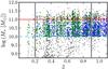Fig. 1

Stellar mass as a function of redshift in the COSMOS field. Red dots are principal galaxies (M_⋆ ≥ 10¹¹ M_⊙) with z_phot in the zCOSMOS area, blue dots are companion galaxies (M_⋆ ≥ 10¹⁰ M_⊙) with z_phot in the COSMOS area, and black dots are the red galaxies (NUV − r⁺ ≥ 3.5) with z_phot in the COSMOS area. We only show a random 15% of the total populations for visualisation purposes. Green squares mark those galaxies in previous populations with a spectroscopic resdhift. The vertical lines mark the lower and upper redshift in our study, while the horizontal ones the mass selection of the principal (solid) and the companion (dashed) samples.

2.1. Definition of the mass-selected samples

We define two samples selected in stellar mass. The first one comprises 2047 principal massive galaxies in the zCOSMOS area, where spectroscopic information is available, with M_⋆ ≥ 10¹¹ M_⊙ ( $M_{⋆} ≳ M_{⋆}^{*}$ $\hbox{$M_{\star} \gtrsim M_{\star}^*$}$ , Ilbert et al. 2010) at 0.1 ≤ z < 1.1. The second sample comprises the 23992 companion galaxies with M_⋆ ≥ 10¹⁰ M_⊙ in the full COSMOS area and in the same redshift range. The mass limit of the companion sample ensures completeness for red galaxies up to z ~ 0.9 (Drory et al. 2009; Ilbert et al. 2010). Because of that, we set z_up = 0.9 as the upper redshift in our study, while z_down = 0.2 to probe enough cosmological volume. However, our methodology takes into account the photometric redshift errors (see Sect. 3, for details), so we must include in the samples not only the sources with z < z_up, but also those sources with z − 2σ_phot < z_up in order to ensure completeness in redshift space. Because of this, we set the maximum and minimum redshift of the catalogues to z_min = 0.1 and z_max = 1.1. We show the mass distribution of our samples as a function of z in Fig. 1, and we assume our samples as volume-limited mass-selected in the following.

Our final goal is to measure the merger fraction and rate of massive ETGs, but our principal sample comprises ETGs, spirals and irregulars. We segregate morphologically our principal sample thanks to the morphological classification defined in Tasca et al. (2009). Their method use as morphological indicator the distance of the galaxies in the multi-space C − A − G (Concentration, Asymmetry and Gini coefficient) to the position in this space of a training sample of ~500 eye-ball classified galaxies. These morphological indices were measured in the HST/ACS images of the COSMOS field, taken through the wide F814W filter (Koekemoer et al. 2007). The galaxies in the training sample were classified into ellipticals, lenticulars, spirals of all types (Sa, Sb, Sc, Sd), irregulars, point-like and undefined sources, and then these classes were grouped into early-type (E, S0), spirals (Sa, Sb, Sc, Sd) and irregular galaxies. It is this coarser classification that was considered in building the training set. The unclassified objects were not used for the training. We refer the reader to Tasca et al. (2009) for further details. The morphological classification in the COSMOS field is reliable for galaxies brighter than i⁺ < 24, and all our principal galaxies are brighter than i⁺ < 23.5 up to z = 1. According to the classification presented in Tasca et al. (2009) our principal sample comprises 1285 (63%) ETGs (E/S0) and 632 (31%) spiral galaxies. The remaining 6% sources are half irregulars (65 sources) and half massive galaxies without morphological classification (65 sources). We stress that the classification of the principal sample is exclusively morphological, without taking into account any additional colour information, i.e., some of our ETGs could be star-forming. We checked that ~95% of our massive ETGs are also quiescent (they have a rest-frame, dust reddening corrected colour NUV − r⁺ ≥ 3.5, Ilbert et al. 2010). Regarding the companion sample, we do not attempt to segregate it morphologically because the morphological classification is not reliable for all companion galaxies (see Sect. 4.3, for details).

We used C, A and G automatic indices to classify morphologically the principal galaxy of the close pair systems. However, these indices are affected by interactions, e.g., the asymmetry increases, and we could misclassify ETGs and spirals as irregular galaxies. Hernández-Toledo et al. (2005, 2006) study how these morphological indices vary on major interactions in the local universe. They find that ETGs are slightly affected by interactions and that interacting ETGs do not reach the loci of irregular galaxies in the C − A space. However, spiral galaxies are strongly affected by interactions and they can be classified as irregulars by automatic methods. Thus, we do not expect misclassifications in our ETGs sample, while some of our irregular galaxies can be interacting spirals. This is in fact observed by Kampczyk et al. (2011) in the 10 k zCOSMOS sample. They find that the fraction of ETGs in close pairs is similar to that in the underlying non-interacting population, while the fraction of spirals/irregulars in close pairs is lower/higher than expected. However, the sum of spirals and irregulars is similar to that in the underlying population, suggesting a spiral to irregular transformation due to interactions.

In summary, the morphology of ETGs is slightly affected by interactions, while some spirals could be classified as irregulars during a merger. Because of this, we define late-type galaxies (LTGs) as spirals + irregulars, thus avoiding any bias due to morphological transformations during the merger process. We show some representative examples of our massive ETGs and LTGs in Fig. 2. 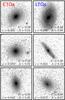The mean mass of both ETGs and LTGs is similar, $M_{⋆} ~ 10^{11.2} M_{⊙}$ $\hbox{$\overline{M_{\star}} \sim 10^{11.2}\ M_{\odot}$}$ .

Fig. 2

Examples of the typical ETGs (left) and LTGs (right) with M_⋆ ≥ 10¹¹ M_⊙ in the COSMOS field. The postage stamps show a 30 h^-1 kpc × 30 h^-1 kpc area of the HST/ACS F814W image at the redshift of the source, with the North on the top and the East on the left. The pixel scale of the HST/ACS image is 0.05′′. The grey scale ranges from 0.5σ_sky to 150σ_sky, where σ_sky is the dispersion of the sky around the source. The redshift, the concentration (C) and the asymmetry (A) of the sources are labelled in the panels.

2.2. Dependence of the photometric errors on stellar mass

The quality of the photometric redshifts in COSMOS decreases for faint objects in the i⁺ band (Ilbert et al. 2009). In this section we study in details how redshift errors depend on the mass of the sources, since this imposes limits on our ability of measure reliable merger fractions in photometric catalogues (Sect. 3.2). As shown by Ilbert et al. (2010), we can estimate the photometric redshift error (σ_{z_phot}) from the Probability Distribution Function of the photometric redshift fit. In Fig. 3 we show the median Δ_z ≡ σ_{z_phot}/(1 + z_phot) of galaxies with different stellar masses, from M_⋆ ≥ 10¹¹ M_⊙ (massive galaxies) to 10¹⁰ M_⊙ ≤ M_⋆ < 10^10.2 M_⊙ (low-mass galaxies) in bins of 0.2 dex.

Massive galaxies are bright in the whole redshift range under study. Thus, their photometric errors are small up to z ~ 1, Δ_z ~ 0.005. On the other hand, low-mass galaxies are fainter at high redshift than their local counterparts, so their their photometric errors increase with z and reach Δ_z ~ 0.015 at z ~ 1. We study separately the photometric errors of low-mass red and blue galaxies. We took as red galaxies those with SED (rest-frame, dust reddening corrected) colour NUV − r⁺ ≥ 3.5, while as blue those with NUV − r⁺ < 3.5 (see Ilbert et al. 2010, for details). Blue galaxies also have Δ_z ~ 0.015 up to z ~ 1, while red galaxies have higher photometric redshift errors, with Δ_z ~ 0.020 at z = 0.95 and Δ_z ~ 0.040 at z = 1.05. This different behaviour can be explained by the different mass-to-light ratio (M_⋆/L) of both populations. Faint (i⁺ ~ 25) blue galaxies, whose photometric errors are higher, reach masses as low as M_⋆ ~ 10^8.5 M_⊙ at z ~ 1. On the other hand, we are in the detection limit for red galaxies at these redshifts (red galaxies have i⁺ ~ 25 at z ~ 1, Sect. 2.1), explaining their high photometric redshift errors. Similar trends in the COSMOS photometric redshift errors were found by George et al. (2011). In Sect. 3.2 we prove that our methodology is able to recover reliable merger fractions in COSMOS samples with Δ_z ≲ 0.040, as those in our study.

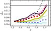Fig. 3

Δ_z as a function of redshift in the mass-selected sample, from M_⋆ ≥ 10¹¹ M_⊙ (thiner line) to 10¹⁰ M_⊙ ≤ M_⋆ < 10^10.2 M_⊙ (thicker line) galaxies in bins of 0.2 dex. The black solid line marks the photometric errors of blue galaxies in the lower mass bin, while the black dashed line is for red galaxies in the same mass bin. The vertical line marks the higher redshift in our samples, z_max = 1.1. The horizontal line marks the median Δ_z for low-mass galaxies at the high redshift end of our sample 1.0 ≤ z < 1.1, Δ_z = 0.015.

3. Close pairs using photometric redshifts

The linear distance between two sources can be obtained from their projected separation, r_p = θd_A(z_i), and their rest-frame relative velocity along the line of sight, Δv = c | z_j − z_i | /(1 + z_i), where z_i and z_j are the redshift of the principal (more luminous/massive galaxy in the pair) and companion galaxy, respectively; θ is the angular separation, in arcsec, of the two galaxies on the sky plane; and d_A(z) is the angular scale, in kpc/arcsec, at redshift z. Two galaxies are defined as a close pair if $r_{p}^{\min} \leq r_{p} \leq r_{p}^{\max}$ $\hbox{$r_{\rm p}^{\rm min} \leq r_{\rm p} \leq r_{\rm p}^{\rm max}$}$ and Δv ≤ Δv^max. The lower limit in r_p is imposed to avoid seeing effects. We used $r_{p}^{\min} = 10 h^{-1}$ $\hbox{$r_{\rm p}^{\rm min} = 10~h^{-1}$}$ kpc, $r_{p}^{\max} = 30 h^{-1}$ $\hbox{$r_{\rm p}^{\rm max} = 30~h^{-1}$}$ kpc, and Δv^max = 500 km s^-1. With these constraints 50 − 70% of the selected close pairs will finally merge (Patton et al. 2000; Patton & Atfield 2008; Lin et al. 2004; Bell et al. 2006). The PSF of the COSMOS ground-based images is 1.5″ (Capak et al. 2007), which corresponds to ~8 h^-1 kpc in our cosmology at z ~ 0.9. To ensure well deblended sources and to minimise colour contamination, we fixed $r_{p}^{\min}$ $\hbox{$r_{\rm p}^{\rm min}$}$ to 10 h^-1 kpc (θ ≳ 2″). On the other hand, we set $r_{p}^{\max}$ $\hbox{$r_{\rm p}^{\rm max}$}$ to 30 h^-1 kpc to ensure reliable merger fractions in our study (see Sect. 3.2, for details).

To compute close pairs we defined a principal and a companion sample (Sect. 2.1). The principal sample comprises the more massive galaxy of the pair, and we looked for those galaxies in the companion sample that fulfil the close pair criterion for each galaxy of the principal sample. If one principal galaxy has more than one close companion, we took each possible pair separately (i.e., if the companion galaxies B and C are close to the principal galaxy A, we study the pairs A-B and A-C as independent). In addition, we imposed a mass difference between the pair members. We denote the ratio between the mass of the principal galaxy, M_⋆ ,1, and the companion galaxy, M_⋆ ,2, as $μ \equiv \frac{M_{⋆, 2}}{M_{⋆, 1}}$ $\begin{equation} \mu \equiv \frac{M_{\star,2}}{M_{\star,1}} \end{equation}$ (1)and looked for those systems with M_⋆ ,2 ≥ μM_⋆ ,1. We define as major companions those close pairs with μ ≥ 1/4, while minor companions those with 1/10 ≤ μ < 1/4.

With the previous definitions the merger fraction is 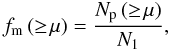$f_{m} (\geq μ) = \frac{N_{p} (\geq μ)}{N_{1}},$ $\begin{equation} f_{\rm m}\,(\geq\! \mu) = \frac{N_{\rm p}\,(\geq\! \mu)}{N_{1}},\label{ncspec} \end{equation}$ (2)where N₁ is the number of sources in the principal sample, and N_p the number of principal galaxies with a companion that fulfil the close pair criterion for a given μ. This definition applies to spectroscopic volume-limited samples. Our samples are volume-limited, but combine spectroscopic and photometric redshifts. In a previous work, López-Sanjuan et al. (2010a) developed a statistical method to obtain reliable merger fractions from photometric catalogues. We recall the main points of this methodology below, while we study its limits when applied to our COSMOS photometric catalogue in Sect. 3.2.

We used the following procedure to define a close pair system in our photometric catalogue (see López-Sanjuan et al. 2010a, for details): first we search for close spatial companions of a principal galaxy, with redshift z₁ and uncertainty σ_z₁, assuming that the galaxy is located at z₁ − 2σ_z₁. This defines the maximum θ possible for a given $r_{p}^{\max}$ $\hbox{$r_{\rm p}^{\rm max}$}$ in the first instance. If we find a companion galaxy with redshift z₂ and uncertainty σ_z₂ in the range $r_{p} \leq r_{p}^{\max}$ $\hbox{$r_{\rm p} \leq r_{\rm p}^{\rm max}$}$ and with a given mass with respect to the principal galaxy, then we study both galaxies in redshift space. For convenience, we assume below that every principal galaxy has, at most, one close companion. In this case, our two galaxies could be a close pair in the redshift range $[z^{-}, z^{+}] = [z_{1} - 2 σ_{z_{1}}, z_{1} + 2 σ_{z_{1}}] \cap [z_{2} - 2 σ_{z_{2}}, z_{2} + 2 σ_{z_{2}}] .$ $\begin{equation} [z^{-},z^{+}] = [z_1 - 2\sigma_{z_1}, z_1 + 2\sigma_{z_1}] \cap [z_2- 2\sigma_{z_2}, z_2 + 2\sigma_{z_2}]. \end{equation}$ (3)Because of variation in the range [z⁻,z⁺] of the function d_A(z), a sky pair at z₁ − 2σ_z₁ might not be a pair at z₁ + 2σ_z₁. We thus impose the condition $r_{p}^{\min} \leq r_{p} \leq r_{p}^{\max}$ $\hbox{$r_{\rm p}^{\rm min} \leq r_{\rm p} \leq r_{\rm p}^{\rm max}$}$ at all z ∈ [z⁻,z⁺] , and redefine this redshift interval if the sky pair condition is not satisfied at every redshift. After this, our two galaxies define the close pair system k in the redshift interval $[z_{k}^{-}, z_{k}^{+}]$ $\hbox{$[z^{-}_k,z^{+}_k]$}$ , where the index k covers all the close pair systems in the sample.

The next step is to define the number of pairs associated at each close pair system k. For this, we suppose in the following that a galaxy i in whatever sample is described in redshift space by a probability distribution P_i (z_i | η_i), where z_i is the source’s redshift and η_i are the parameters that define the distribution. If the source i has a photometric redshift, we assume that 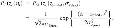$\begin{matrix} P_{i} (z_{i} | η_{i}) & = & P_{G} (z_{i} | z_{phot,i}, σ_{z_{phot,i}}) \\ = \end{matrix}$ $\begin{eqnarray} P_i\, (z_i\, |\, \eta_i) &=& P_{\rm G}\, (z_i\, |\, z_{{\rm phot},i},\sigma_{z_{{\rm phot},i}}) \nonumber\\ &= &\frac{1}{\sqrt{2\pi}\sigma_{z_{{\rm phot},i}}}\exp\left\{{-\frac{(z_i-z_{{\rm phot},i})^2}{2\sigma_{z_{{\rm phot},i}}^2}}\right\}\label{zgauss}, \end{eqnarray}$ (4)while if the source has a spectroscopic redshift $P_{i} (z_{i} | η_{i}) = P_{D} (z_{i} | z_{spec,i}) = δ (z_{i} - z_{spec,i}),$ $\begin{equation} P_i\, (z_i\, |\, \eta_i) = P_{\rm D}\, (z_i\, |\, z_{{\rm spec},i}) = \delta(z_i - z_{{\rm spec},i}), \end{equation}$ (5)where δ(x) is delta’s Dirac function. With this distribution we are able to statistically treat all the available information in z space and define the number of pairs at redshift z₁ in system k as 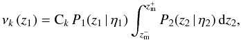$ν_{k} (z_{1}) = C_{k} P_{1} (z_{1} | η_{1}) \int_{z_{m}^{-}}^{z_{m}^{+}} P_{2} (z_{2} | η_{2}) d z_{2},$ $\begin{equation} \nu_{k}\,(z_1) = {\rm C}_k\, P_1 (z_1\, |\, \eta_1) \int_{z_{\rm m}^{-}}^{z_{\rm m}^{+}} P_2 (z_2\, |\, \eta_2)\, {\rm d}z_2,\label{nuj} \end{equation}$ (6)where $z_{1} \in [z_{k}^{-}, z_{k}^{+}]$ $\hbox{$z_1 \in [z^{-}_k,z^{+}_k]$}$ , the integration limits are $\begin{matrix} z_{m}^{-} = z_{1} (1 - Δ v^{\max} / c) - Δ v^{\max} / c, \\ z_{m}^{+} = z_{1} (1 + Δ v^{\max} / c) + Δ v^{\max} / c, \end{matrix}$ $\begin{eqnarray} z_{\rm m}^{-} = z_1(1-\Delta v^{\rm max}/c) - \Delta v^{\rm max}/c,\\ z_{\rm m}^{+} = z_1(1+\Delta v^{\rm max}/c) + \Delta v^{\rm max}/c, \end{eqnarray}$ 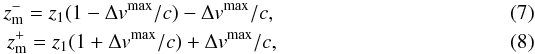the subindex 1 [2] refers to the principal [companion] galaxy in k system, and the constant C_k normalises the function to the total number of pairs in the interest range 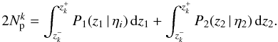$2 N_{p}^{k} = \int_{z_{k}^{-}}^{z_{k}^{+}} P_{1} (z_{1} | η_{i}) d z_{1} + \int_{z_{k}^{-}}^{z_{k}^{+}} P_{2} (z_{2} | η_{2}) d z_{2} .$ $\begin{equation} 2 N_{\rm p}^k = \int_{z_k^{-}}^{z_k^{+}} P_1 (z_1\, |\, \eta_i)\, {\rm d}z_1 + \int_{z_k^{-}}^{z_k^{+}} P_2 (z_2\, |\, \eta_2)\, {\rm d}z_2. \end{equation}$ (9)Note that ν_k = 0 if $z_{1} < z_{k}^{-}$ $\hbox{$z_1 < z_k^-$}$ or $z_{1} > z_{k}^{+}$ $\hbox{$z_1 > z_k^+$}$ . The function ν_k (Eq. (6)) tells us how the number of pairs in the system k, $N_{p}^{k}$ $\hbox{$N_{\rm p}^k$}$ , are distributed in redshift space. The integral in Eq. (6) spans those redshifts in which the companion galaxy has Δv ≤ Δv^max for a given redshift of the principal galaxy.

With previous definitions, the merger fraction in the interval z_r,l = [z_l,z_l + 1) is $f_{m,l} = \frac{\sum_{k} \int_{z_{l}}^{z_{l + 1}} ν_{k} (z_{1}) d z_{1}}{\sum_{i} \int_{z_{l}}^{z_{l + 1}} P_{i} (z_{i} | η_{i}) d z_{i}},$ $\begin{equation} f_{{\rm m},l} = \frac{\sum_k \int_{z_l}^{z_{l+1}}{\nu_k(z_1)}\, {\rm d}z_1}{\sum_i \int_{z_l}^{z_{l+1}} P_i\, (z_i\, |\, \eta_i)\, {\rm d}z_i},\label{ncphot} \end{equation}$ (10)where the index l spans the redshift bins defined over the redshift range under study. If we integrate over the whole redshift space, z_r = [0,∞), Eq. (10) becomes $f_{m} (\geq μ) = \frac{\sum_{k} N_{p}^{k} (\geq μ)}{N_{1}},$ $\begin{equation} f_{{\rm m}}\,(\geq \mu) = \frac{\sum_k N_{\rm p}^k\,(\geq \!\mu)}{N_1},\label{ncphot2} \end{equation}$ (11)where $\sum_{k} N_{p}^{k}$ $\hbox{$\sum_k N_{\rm p}^k$}$ is analogous to N_p in Eq. (2). In order to estimate the statistical error of f_m,l, denoted σ_stat,l, we used the jackknife technique (Efron 1982). We computed partial standard deviations, δ_k, for each system k by taking the difference between the measured f_m,l and the same quantity with the kth pair removed for the sample, $f_{m,l}^{k}$ $\hbox{$f_{{\rm m},l}^k$}$ , such that $δ_{k} = f_{m,l} - f_{m,l}^{k}$ $\hbox{$\delta_k = f_{{\rm m},l} - f_{{\rm m},l}^k$}$ . For a redshift range with N_p systems, the variance is given by $σ_{stat,l}^{2} = [(N_{p} - 1) \sum_{k} δ_{k}^{2}] / N_{p}$ $\hbox{$\sigma_{{\rm stat},l}^2 = [(N_{\rm p}-1) \sum_k \delta_k^2]/N_{\rm p}$}$ . When N_p ≤ 5 we used instead the Bayesian approach of Cameron (2011), that provides accurate asymmetric confidence intervals in these low statistical cases. We checked that for N_p > 5 both jackknife and Bayesian methods provide similar statistical errors within 10%.

3.1. Dealing with border effects

When we search for close companions near to the edges of the images it may happen that a fraction of the search volume is outside of the surveyed area, lowering artificially the number of companions. To deal with this we selected as principal galaxies those in the zCOSMOS area, i.e., in the central 1.6 deg², while we selected as companions those in the whole photometric COSMOS area. This maximise the spectroscopic fraction of the principal sample and ensures that we have companions inside all the searching volume.

3.2. Testing the methodology with 20 k spectroscopic sources

Following López-Sanjuan et al. (2010a), we test in this section if we are able to obtain reliable merger fractions from our COSMOS photometric catalogue. For this, we study the merger fraction f_m in the zCOSMOS-bright 20 k sample. The merger fraction in the 10 k sample was studied in details by de Ravel et al. (2011) and Kampczyk et al. (2011). We defined f_spec as the fraction of sources on a given sample with spectroscopic redshift. The 20 k sample has f_spec = 1, while the COSMOS photometric catalogue has f_spec = 0.34 for i⁺ ≤ 22.5 galaxies. In this section we only use the N = 10542 sources at 0.2 ≤ z < 0.9 with a high reliable spectroscopic redshift from the 20 k sample.

To test our method at intermediate f_spec, we created synthetic catalogues by assigning their measured z_phot and σ_{z_phot} to N(1 − f_spec) random sources of the 20 k sample (we denote this case as S = 1 in the following). To explore different values of Δ_z, we assigned to the previous random sources a redshift as drawn for a Gaussian distribution with median z_phot and $σ^{2} = (S^{2} - 1) σ_{z_{phot}}^{2}$ $\hbox{$\sigma^{2} = (S^2-1)\,\sigma_{z_{\rm phot}}^2$}$ , where S > 1 is the factor by which we increase the initial Δ_z of the sample. In this case, the redshift error of the source is set to Sσ_{z_phot}. Then, we measured $δ f_{m} \equiv \frac{f_{m}^{syn}}{f_{m}^{20 k}} - 1,$ $\begin{equation} \delta f_{\rm m} \equiv \frac{f_{\rm m}^{\rm syn}}{f_{\rm m}^{\rm 20~k}} - 1, \end{equation}$ (12)where $f_{m}^{20 k}$ $\hbox{$f_{\rm m}^{\rm 20~k}$}$ is the measured merger fraction in the 20 k spectroscopic sample at 0.2 ≤ z < 0.9 without imposing any mass or luminosity difference and $f_{m}^{syn}$ $\hbox{$f_{\rm m}^{\rm syn}$}$ is the merger fraction from the synthetic samples in the same redshift range. When S > 1, we repeated the process ten times and averaged the results.

We explored several cases with our synthetic catalogues. For example, we assumed that all sources in the synthetic principal catalogue (subindex 1) and in the companion one (subindex 2) have a photometric redshift, f_spec,1 = f_spec,2 = 0, and that Δ_z,1 = Δ_z,2 = 0.007 (S₁ = S₂ = 1). We also considered more realistic cases, as f_spec,1 = 0.3 and Δ_z,1 = 0.007 (S₁ = 1) for principals, and f_spec,2 = 0 and Δ_z,2 = 0.042 (S₂ = 6) for companions. We found that δf_m is higher than 10% for $r_{p}^{\max} = 30 h^{-1}$ $\hbox{$r_{\rm p}^{\rm max} = 30~h^{-1}$}$ kpc close pairs for Δ_z,2 ≳ 0.05 (S₂ ≳ 7) and realistic values of Δ_z,1. We checked that | δf_m | ≲ 10% for Δ_z,2 ≤ 0.04 and $r_{p}^{\max} = 30 h^{-1}$ $\hbox{$r_{\rm p}^{\rm max} = 30~h^{-1}$}$ kpc, justifying the upper limit Δ_z = 0.04 imposed in Sect. 2.2. For higher $r_{p}^{\max}$ $\hbox{$r_{\rm p}^{\rm max}$}$ the method overestimates the merger fraction by about 50% in the Δ_z,2 = 0.04 case. Because we are interested on faint companions, we set $r_{p}^{\max} = 30 h^{-1}$ $\hbox{$r_{\rm p}^{\rm max} = 30~h^{-1}$}$ kpc in the following to ensure reliable merger fractions.

On the other hand, we found that the σ_stat of the $f_{m}^{syn}$ $\hbox{$f_{\rm m}^{\rm syn}$}$ is ~ 5% of the measured value, i.e., two times lower than the estimated | δf_m | ~ 10%. Because of this, and to ensure reliable uncertainties in the merger fractions, we impose a minimum error in f_m of 10%, and we take as final merger fraction error σ_{f_m} = max(0.1f_m,σ_stat).

In the next section we test further our methodology by comparing the merger fraction from a spectroscopic survey (f_spec = 1) against that in COSMOS from our photometric catalogue.

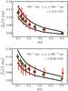Fig. 4

Merger fraction of $M_{B}^{e} \leq - 20$ $\hbox{$M_{B}^{\rm e} \leq -20$}$ galaxies as a function of luminosity difference in the B-band, μ_B, at z ∈ [0.2,0.65) (top) and z ∈ [0.65,0.95) (bottom) for 10 h^-1 kpc ≤ r_p ≤ 30 h^-1 kpc close pairs. Diamonds are from present work in COSMOS (photometric catalogue) while dots are from VVDS-Deep (LS11, spectroscopic catalogue). The black solid lines in both panels show the maximum and minimum merger fractions, including 1σ_{f_m} errors, when we split the COSMOS field in VVDS-Deep size subfields (~0.5 deg²).

3.3. Comparison with merger fractions in VVDS-Deep: cosmic variance effect

In a previous work in VVDS-Deep, LS11 measured the merger fraction of $M_{B}^{e} \leq - 20$ $\hbox{$M_{B}^{\rm e} \leq -20$}$ galaxies with spectroscopic redshifts, where $M_{B}^{e} = M_{B} + Qz$ $\hbox{$M_{B}^{\rm e} = M_{B} + Qz$}$ and Q = 1.1 accounts for the evolution of the luminosity function with redshift, as a function of luminosity difference in the B-band, μ_B = L_B,2/L_B,1. As an additional test of our methodology, in this section we compare the merger fraction in the COSMOS photometric catalogue with that measured by LS11 down to μ_B = 1/10, reaching the minor merger regime in which we are interested on. To minimise the systematic biases, we used the same redshift ranges, z_r,1 = [0.2,0.65) and z_r,2 = [0.65,0.95), close pair definition ( $r_{p}^{\max} = 30 h^{-1}$ $\hbox{$r_{\rm p}^{\rm max} = 30~h^{-1}$}$ kpc), principal sample ( $M_{B}^{e} \leq - 20$ $\hbox{$M_{B}^{\rm e} \leq -20$}$ ), and companion sample ( $M_{B}^{e} \leq - 17.5$ $\hbox{$M_{B}^{\rm e} \leq -17.5$}$ ) than LS11. We checked that the photometric redshift errors are Δ_z ≲ 0.04 up to z ~ 0.95 for faint companion galaxies (see Sect. 3.2). Note that LS11 use $r_{p}^{\min} = 5 h^{-1}$ $\hbox{$r_{\rm p}^{\rm min} = 5~h^{-1}$}$ kpc, while we take $r_{p}^{\min} = 10 h^{-1}$ $\hbox{$r_{\rm p}^{\rm min} = 10~h^{-1}$}$ kpc. Hence, we recomputed the merger fractions in VVDS-Deep for $r_{p}^{\min} = 10 h^{-1}$ $\hbox{$r_{\rm p}^{\rm min} = 10~h^{-1}$}$ kpc. We show the merger fractions from COSMOS and VVDS-Deep for different values of μ_B in Fig. 4.

We find that VVDS-Deep and COSMOS merger fractions are in excellent agreement in the first redshift range, while in the second redshift range some discrepancies exist, with the merger fraction in COSMOS being higher than in VVDS-Deep at μ ≲ 1/5. However, both studies are compatible within error bars. Note that merger fraction uncertainties in COSMOS are ~3 times lower than in VVDS-Deep because of the higher number of principals in COSMOS. We checked the effect of comic variance in this comparison. For that, we split the zCOSMOS area in several VVDS-Deep size (~0.5 deg²) subfields and measured the merger fraction in these subfields. The maximum and minimum values of f_m in these subfields, including 1σ_{f_m} errors, are marked in Fig. 4 with solid lines. We find that, within 1σ_{f_m}, there is a zCOSMOS subfield with merger properties similar to the VVDS-Deep field. Because the zCOSMOS subfields are contiguous, this exercise provides a lower limit to the actual cosmic variance in the COSMOS field (e.g., Moster et al. 2011). Hence, we conclude that our methodology is able to recover reliable minor merger fractions from photometric samples in the COSMOS field.

4. The merger fraction of massive ETGs in the COSMOS field

The final goal of the present paper is to estimate the role of mergers (minor and major) in the mass assembly and size evolution of massive ETGs. To facilitate future comparison, we present first the merger properties of the global massive population in Sect. 4.1. Then, we focus in the ETGs population in Sect. 4.2.

The evolution of the merger fraction with redshift up to z ~ 1.5 is well parametrised by a power-law function (e.g., Le Fèvre et al. 2000; López-Sanjuan et al. 2009; de Ravel et al. 2009), 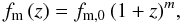$f_{m} (z) = f_{m, 0} (1 + z)^{m},$ $\begin{equation} f_{\rm m}\,(z) = f_{\rm m,0}\,(1+z)^{m}, \label{ffzeq} \end{equation}$ (13)so we take this parametrisation in the following.

4.1. The merger fraction of the global massive population

We summarise the minor, major and total merger fractions for M_⋆ ≥ 10¹¹ M_⊙ galaxies in the COSMOS field in Table 1 and we show them in Fig. 5. We defined five redshift bins between z_down = 0.2 and z_up = 0.9 both for minor and major mergers. The ranges 0.3 < z < 0.375, 0.7 < z < 0.75 and 0.825 < z < 0.85 are dominated by Large Scale Structures (LSS, Kovač et al. 2010), so we use these LSS as natural boundaries in our study. This minimises the impact of LSS in our measurements, since the merger fraction depends on environment (Lin et al. 2010; de Ravel et al. 2011; Kampczyk et al. 2011). We identify a total of 56.2 major mergers and 71.1 minor ones at 0.2 ≤ z < 0.9. Note that the number of mergers can take non integer values because of the weighting scheme used in our methodology (Sect. 3). We compare the previous number of mergers (measured as $Σ_{k} N_{p}^{k}$ $\hbox{$\Sigma_{k} N_{\rm p}^{k}$}$ , Eq. (11)) with the total number of close pair systems (N_p), obtaining that the fraction of real close pairs over the total number of systems is ~65%. We find that

The minor merger fraction is nearly constant with redshift,f_mm ~ 0.051. The least-squares fit to the minor merger fraction data is $f_{mm} = (0.052 \pm 0.009) (1 + z)^{- 0.1 \pm 0.3} .$ $\begin{equation} f_{\rm mm} = (0.052 \pm 0.009) (1+z)^{-0.1 \pm 0.3}. \end{equation}$ (14)The negative value of the power-law index implies that the minor merger fraction decreases slightly with redshift, but it is consistent with a null evolution (m_mm = 0). This confirms the trend found by LS11 for bright galaxies, and by Jogee et al. (2009) and Lotz et al. (2011) for less massive (M_⋆ ≳ 10¹⁰ M_⊙) galaxies, and extend it to the high mass regime.

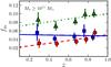
Fig. 5

Major (dots), minor (squares) and total (major + minor, triangles) merger fraction of M_⋆ ≥ 10¹¹ M_⊙ galaxies as a function of redshift in the COSMOS field. Dashed, solid and dott-dashed curves are the least-squares best fit of a power-law function, f_m ∝ (1 + z)^m, to the major (m_MM = 1.4), minor (m_mm = −0.1) and total (m_m = 0.6) merger fraction data, respectively.

The major merger fraction of massive galaxies increases with redshift as $f_{MM} = (0.019 \pm 0.003) (1 + z)^{1.4 \pm 0.3} .$ $\begin{equation} f_{\rm MM} = (0.019 \pm 0.003) (1+z)^{1.4 \pm 0.3}.\label{ffMMeq} \end{equation}$ (15)This increase with z contrasts with the nearly constant minor merger fraction. In Fig. 6 we compare our measurements with those from the literature for massive galaxies and for $r_{p}^{\max} ~ 30 h^{-1}$ $\hbox{$r_{\rm p}^{\rm max} \sim 30~h^{-1}$}$ kpc close pairs. de Ravel et al. (2011) measure the major merger fraction by r_p ≤ 30 h^-1 kpc spectroscopic close pairs in the 10 k zCOSMOS sample, so their sample is included in ours. Because they assume a different inner radius than us, we apply a factor 2/3 to their original values (see Sect. 5, for details). Both merger fractions are in good agreement, supporting our methodology. Note that our uncertainties are lower by a factor of three than those in de Ravel et al. (2011) because our principal sample is a factor of four larger than theirs. Xu et al. (2012) measure the merger fraction from photometric close pairs also in the COSMOS field. They provide the fraction of galaxies in close pairs with μ ≥ 1/2.5, so we apply a factor 0.7 to obtain the number of close pairs (this is the fraction of principal galaxies in their massive sample) and a factor 1.6 to estimate the number of μ ≥ 1/4 systems (the merger fraction depends on μ as f_m ∝ μ^s, as shown by LS11, and s = −0.95 for massive galaxies in COSMOS, Sect. 6.2). On the other hand, Bundy et al. (2009) and Bluck et al. (2009) measure the major (μ ≥ 1/4) merger fraction in GOODS⁴ (Great Observatories Origins Deep Survey, Giavalisco et al. 2004) and Palomar/DEEP2 (Conselice et al. 2007) surveys, respectively. These studies are also in good agreement with our values, with the point at z = 0.8 from Bluck et al. (2009) being the only discrepancy. The least-squeres fit to all the close pair studies in Fig. 6 yields similar parameters to those from our COSMOS data alone, Eq. (15).

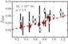
Fig. 6

Major (μ ≥ 1/4) merger fraction for M_⋆ ≥ 10¹¹ M_⊙ galaxies from $r_{p}^{\max} ~ 30 h^{-1}$ $\hbox{$r_{\rm p}^{\rm max} \sim 30~h^{-1}$}$ kpc close pairs. The dots are from present work, triangles are form de Ravel et al. (2011) in the zCOSMOS 10 k sample, squares from Xu et al. (2012) in the COSMOS field, pentagons from Bluck et al. (2009) in the Palomar/DEEP2 survey, and diamonds from Bundy et al. (2009) in the GOODS fields. Some points are slightly shifted when needed to avoid overlap. The dashed line is the least-squares best fit of a power-law function, f_MM ∝ (1 + z)^1.4, to the major merger fraction data in the present work.

For completeness, if Fig. 7 we compare our major merger fractions with other works that are either based on morphological criteria or come from luminosity-selected samples. Regarding morphological studies, Bridge et al. (2010) provide the major merger fraction of M_⋆ ≳ 5 × 10¹⁰ M_⊙ galaxies in two CFHTLS⁵ (Canada-France-Hawaii Telescope Legacy Survey, Coupon et al. 2009) Deep fields, including the COSMOS field. They perform a visual classification of the sources, finding 286 merging systems of that mass. In their work, Jogee et al. (2009) estimate a lower limit of the major merger fraction of M_⋆ ≥ 2.5 × 10¹⁰ M_⊙ galaxies in the GEMS⁶ (Galaxy Evolution From Morphology And SEDs, Rix et al. 2004) survey. We cannot compare directly the merger fractions from these two morphological studies with ours because of the different methodologies (e.g., Bridge et al. 2010; Lotz et al. 2011). Thus, we translate their merger rates into the expected close pair fraction following the prescriptions in Sect. 5. Giving the uncertainties in the merger time scales of both methods and the difficulties to assign a precise mass ratio μ to the merger candidates in morphological studies, the merger fractions from Bridge et al. (2010) and Jogee et al. (2009) are in nice agreement with our results. Kartaltepe et al. (2007) estimate the merger fraction of luminous galaxies (L_V ≤ −19.8) in the COSMOS field. They take these luminous galaxies to define the principal and the companion sample, i.e., they are incomplete for low luminosity major companions near the selection boundary. We find that both studies in the COSMOS field are compatible in the common redshift range (0.2 < z < 0.9). The different evolution of the major merger fraction in both works, m = 2.8 in Kartaltepe et al. (2007) vs m = 1.4 in our study, is due to the z > 0.9 data. We conclude that both studies are consistent, even if a direct quantitative comparison is not possible because of the different sample selection and companion definition.

The fit to the total merger fraction is $f_{m} = (0.067 \pm 0.008) (1 + z)^{0.6 \pm 0.3} .$ $\begin{equation} f_{\rm m} = (0.067 \pm 0.008) (1+z)^{0.6 \pm 0.3}. \end{equation}$ (16)This evolution is slower than the major merger one, reflecting the different properties of minor and major mergers. We compare our total merger fractions with others in the literature in Fig. 8. Mármol-Queraltó et al. (2012) study the total merger fraction of massive galaxies by $r_{p}^{\max} = 70 h^{-1}$ $\hbox{$r_{\rm p}^{\rm max} = 70~h^{-1}$}$ kpc close companions. The merger fraction depends on the search radius as $f_{m} \propto r_{p}^{-0.95}$ $\hbox{$f_{\rm m} \propto r_{\rm p}^{-0.95}$}$ (LS11), so we translate the merger fractions provided by Mármol-Queraltó et al. (2012) to our search radius. On the other hand, Newman et al. (2012) measure the merger fraction of M_⋆ ≥ 5 × 10¹⁰ M_⊙ galaxies from $r_{p}^{\max} = 30 h^{-1}$ $\hbox{$r_{\rm p}^{\rm max} = 30~h^{-1}$}$ kpc close pairs. The values from both close pair studies are consistent with ours. Also the results of Williams et al. (2011) suggest a slow/null evolution in the total (μ ≥ 1/10) merger faction of massive galaxies up to z ~ 2.

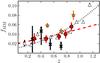
Fig. 7

Major merger fraction as a function of redshift. The dots are from present work for M_⋆ ≥ 10¹¹ M_⊙ galaxies from 10 h^-1 kpc $\leq r_{p}^{\max} \leq 30 h^{-1}$ $\hbox{$\leq r_{\rm p}^{\rm max} \leq 30~h^{-1}$}$ kpc close pairs. The triangles are from Kartaltepe et al. (2007) in the COSMOS field for M_V ≤ − 19.8 galaxies from 5 h^-1 kpc $\leq r_{p}^{\max} \leq 20 h^{-1}$ $\hbox{$\leq r_{\rm p}^{\rm max} \leq 20~h^{-1}$}$ kpc close pairs. The stars are from Bridge et al. (2010) in the CFHTLS by morphological criteria for M_⋆ ≳ 5 × 10¹⁰ M_⊙ galaxies, and crosses are from Jogee et al. (2009) for M_⋆ ≥ 2.5 × 10¹⁰ M_⊙ galaxies by morphological criteria in GEMS (upward arrows mark those points that are lower limits). The dashed line is the least-squares best fit of a power-law function, f_MM ∝ (1 + z)^1.4, to the major merger fraction data in the present work. The dotted line is the evolution from Kartaltepe et al. (2007), f_MM ∝ (1 + z)^2.8.

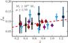
Fig. 8

Total (major + minor, μ ≥ 1/10) merger fraction as a function of redshift. Dots are from the present work in the COSMOS field for M_⋆ ≥ 10¹¹ M_⊙ galaxies, diamonds are from Mármol-Queraltó et al. (2012) for massive galaxies, squares are from Newman et al. (2012) for M_⋆ ≥ 5 × 10¹⁰ M_⊙ galaxies, crosses are from Jogee et al. (2009) for M_⋆ ≥ 2.5 × 10¹⁰ M_⊙ galaxies by morphological criteria, and inverted triangles are from Lotz et al. (2011) for M_⋆ ≥ 10¹⁰ M_⊙ galaxies by morphological criteria. The dashed line is the least-squares best fit of a power-law function, f_m ∝ (1 + z)^0.6, to the total merger fraction data in the present work.

Regarding morphological studies, Jogee et al. (2009) estimate the total (μ ≥ 1/10) merger fraction of M_⋆ ≥ 2.5 × 10¹⁰ M_⊙ galaxies in the GEMS survey. Their values, f_m ~ 0.08, are consistent with ours. We also show the merger fraction from Lotz et al. (2011) for M_⋆ ≥ 10¹⁰ M_⊙ galaxies in the AEGIS⁷ (All-Wavelength Extended Groth Strip International Survey, Davis et al. 2007) survey. The different methodologies between these works and ours, and the different stellar mass regimes probed, make direct comparisons difficult (see Bridge et al. 2010; Lotz et al. 2011, for a review of this topic). In summary, previous work is compatible with a mild evolution of the total merger fraction, as we observe.

Table 1

Minor, major and total merger fraction of M_⋆ ≥ 10¹¹ M_⊙ galaxies.

4.2. The merger fraction of ETGs

We summarise the minor and major merger fractions for both massive (M_⋆ ≥ 10¹¹ M_⊙) ETGs and LTGs in the COSMOS field in Tables 2 and 3, respectively, while we show them in Fig. 9. We defined five redshift bins between z_down = 0.2 and z_up = 0.9 for ETGs, as for the global population, but only three in the case of LTGs because of the lower number of principal sources. We do not split the companion sample by neither morphology or colour in this section, and we study the properties of the companion galaxies in Sect. 4.3.

We assume m_mm = 0 in the following for the minor merger fraction, as for the global population (Sect. 4.1). The mean minor merger fraction of ETGs is $f_{mm}^{ET} = 0.060$ $\hbox{$f_{\rm mm}^{\rm ET} = 0.060$}$ , while $f_{mm}^{LT} = 0.023$ $\hbox{$f_{\rm mm}^{\rm LT} = 0.023$}$ for LTGs. There is therefore a factor of three difference between the merger fractions of early type and late type populations. LS11 also find a similar result when comparing the minor merger fraction of red and blue bright galaxies.

On the other hand, the major merger fraction of ETGs is also higher than that of LTGs by a factor of two. The fit to the major merger data yields 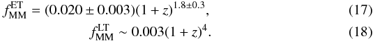$\begin{matrix} f_{MM}^{ET} = (0.020 \pm 0.003) (1 + z)^{1.8 \pm 0.3}, \\ f_{MM}^{LT} ~ 0.003 (1 + z)^{4} . \end{matrix}$ $\begin{eqnarray} f_{\rm MM}^{\rm ET} = (0.020 \pm 0.003) (1+z)^{1.8 \pm 0.3},\\ f_{\rm MM}^{\rm LT} \sim 0.003 (1+z)^{4}. \end{eqnarray}$ Because we only have three data points for LTGs and of the high uncertainty in the first redshift bin, the reported value of m_MM for massive LTGs is only tentative. Nevertheless, that the major merger fraction of LTGs evolves faster than that of ETGs is in agreement with previous studies which compare early-types/red and late-types/blue galaxies (e.g., Lin et al. 2008; de Ravel et al. 2009; Bundy et al. 2009; Chou et al. 2011; LS11).

As shown by Lotz et al. (2011), the merger rate evolution depends on the selection of the sample, with samples selected to prove a constant number density population over cosmic time showing a faster evolution (m ~ 3) than those with a constant mass selection (m ~ 1.5). To check the impact of the selection in the merger fraction of ETGs, we computed the major and minor merger fraction of ETGs with log (M_⋆/M_⊙) ≥ 11.15 − 0.15z (n-selected sample, in the following). As shown by van Dokkum et al. (2010), this provides a nearly constant number-density selection for massive galaxies. We find that the major and minor merger fractions from the n-selected sample are compatible with those from the mass-selected sample. Regarding their evolution, the major merger fraction evolves faster in the n-selected sample, m = 2.5 ± 0.4, that in the mass-selected sample, m = 1.8 ± 0.3, as expected. The minor merger fraction remains the same, f_mm = 0.064 ± 0.006 (n-selected sample) vs. f_mm = 0.060 ± 0.008 (mass-selected sample). In addition, we checked that the results presented in Sect. 6 remain the same when we use the merger fractions from the n-selected sample instead of those from the mass-selected one. Therefore, we conclude that the selection of the massive ETGs sample has limited impact in our results.

In summary, the merger fraction of massive (M_⋆ ≥ 10¹¹ M_⊙) ETGs, both major and minor, is higher by a factor of 2 − 3 than that of massive LTGs (see also Mármol-Queraltó et al. 2012, for a similar result). We estimate the merger rate of ETGs in Sect. 5.

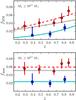Fig. 9

Major (upper panel) and minor (lower panel) merger fractions of M_⋆ ≥ 10¹¹ M_⊙ galaxies as a function of redshift and morphology. Dots are for ETGs, while squares are for LTGs. Dashed (solid) lines are the best fit to the ETGs (LTGs) data, while dotted lines are the fits for the global population.

Table 2

Minor and major merger fraction of ETGs with M_⋆ ≥ 10¹¹ M_⊙.

Table 3

Minor and major merger fraction of LTGs with M_⋆ ≥ 10¹¹ M_⊙.

4.3. Colour properties of companion galaxies

In this section we attempt to identify the types of galaxies in the companion population. As the morphological classification is not reliable for all companions because they are faint, we instead use a colour selection. We took as red (quiescent) companions those with SED (rest-frame, dust reddening corrected) colour NUV − r⁺ ≥ 3.5, while as blue (star-forming) those with NUV − r⁺ < 3.5 (see Ilbert et al. 2010, for details), and we measured the fraction of red companions (f_red) of massive galaxies at 0.2 ≤ z < 0.9.

We find that 62% of the companions of the whole principal sample are red, while ~ 38% are blue. Furthermore, the red fraction remains nearly the same for minor (f_red = 60%) and major (f_red = 64%) companions. When we repeated the previous study focusing on massive ETGs as principals, we find f_red ~ 65%, both for minor and major companions. Because ~95% of our massive ETGs are also red, most of the ETG close pairs are “dry” (i.e., red-red).

5. The merger rate of massive ETGs in the COSMOS field

In this section we estimate the minor (R_mm) and major (R_MM) merger rate, defined as the number of mergers per galaxy and Gyr, of massive ETGs. We recall here the steps to compute the merger rate from the merger fraction, focusing first on the major merger rate.

Following de Ravel et al. (2009), we define the major merger rate as $R_{MM} = f_{MM} C_{p} C_{m} T_{MM}^{-1},$ $\begin{equation} R_{\rm MM} = f_{\rm MM}\,C_{\rm p}\, C_{\rm m}\, T_{\rm MM}^{-1},\label{mrparMM} \end{equation}$ (19)where the factor C_p takes into account the lost companions in the inner 10 h^-1 kpc (Bell et al. 2006) and the factor C_m is the fraction of the observed close pairs that finally merge in a typical time scale T_MM. We take C_p = 3/2. The typical merger time scale depends on $r_{p}^{\max}$ $\hbox{$r_{\rm p}^{\rm max}$}$ and can be estimated by cosmological and N-body simulations. In our case, we compute the major merger time scale from the cosmological simulations of Kitzbichler & White (2008), based on the Millennium simulation (Springel et al. 2005). This major merger time scale refers to major mergers (μ > 1/4 in stellar mass), and depends mainly on $r_{p}^{\max}$ $\hbox{$r_{\rm p}^{\rm max}$}$ and on the stellar mass of the principal galaxy, with a weak dependence on redshift in our range of interest (see de Ravel et al. 2009, for details). Taking log (M_⋆/M_⊙) = 11.2 as the average stellar mass of our principal galaxies with a close companion, we obtain T_MM = 1.0 ± 0.2 Gyr for $r_{p}^{\max} = 30 h^{-1}$ $\hbox{$r_{\rm p}^{\rm max} = 30~h^{-1}$}$ kpc and Δv^max = 500 km s^-1. We assumed an uncertainty of 0.2 dex in the average mass of the principal galaxies to estimate the error in T_MM. This time scale already includes the factor C_m (see Patton & Atfield 2008; Bundy et al. 2009; Lin et al. 2010, LS11), so we take C_m = 1 in the following. In addition, LS11 show that time scales from Kitzbichler & White (2008) are equivalent to those from the N-body/hydrodynamical simulations by Lotz et al. (2010b), and that they account properly for the observed increase of the merger fraction with $r_{p}^{\max}$ $\hbox{$r_{\rm p}^{\rm max}$}$ (see also de Ravel et al. 2009). We stress that these merger time scales have an additional factor of two uncertainty in their normalisation (e.g., Hopkins et al. 2010c; Lotz et al. 2011).

The minor merger rate is $R_{mm} = f_{mm} C_{p} C_{m} T_{mm}^{-1},$ $\begin{equation} R_{\rm mm} = f_{\rm mm}\,C_{\rm p}\, C_{\rm m}\, T_{\rm mm}^{-1},\label{mrparmm} \end{equation}$ (20)where T_mm = Υ × T_MM. Following LS11, we take Υ = 1.5 ± 0.1 from the N-body/hydrodynamical simulations of major and minor mergers performed by Lotz et al. (2010b,a; see also Lotz et al. 2011). As for major mergers, we assume C_p = 3/2 and C_m = 1.

We summarise the major and minor merger rates of massive ETGs in Table 4, and show them in Fig. 10. We parametrise their redshift evolution as $R_{m} (z) = R_{m, 0} (1 + z)^{n} .$ $\begin{equation} R_{\rm m}\,(z) = R_{\rm m,0}\,(1+z)^{n}. \label{mrzeq} \end{equation}$ (21)

Table 4

Minor and major merger rate of ETGs with M_⋆ ≥ 10¹¹ M_⊙.

Assuming n_mm = 0 for minor mergers, as for the merger fraction (Sect. 4.2), we find $R_{mm}^{ET} = 0.060 \pm 0.008 {Gyr}^{-1}$ $\hbox{$R_{\rm mm}^{\rm ET} = 0.060 \pm 0.008\ {\rm Gyr}^{-1}$}$ . The fit to the major merger rate of massive ETGs is $R_{MM}^{ET} = (0.030 \pm 0.006) (1 + z)^{1.8 \pm 0.3} {Gyr}^{-1} .$ $\begin{equation} R_{\rm MM}^{\rm ET} = (0.030 \pm 0.006)\,(1+z)^{1.8 \pm 0.3}\ {\rm Gyr}^{-1}.\label{rMMet} \end{equation}$ (22)Our results imply that the minor merger rate is higher than the major merger one at z ≲ 0.5. In addition, the minor and major merger rates of massive ETGs are ~20% higher than for the global population.

In Fig. 10 we also show the minor and major merger rates of red bright galaxies measured by LS11. We find that red galaxies have similar merger rates, both minor and major, than our massive ETGs. This suggests that massive red sequence galaxies have similar merger properties: nearly 95% of our ETGs are red, while the mean mass of the red galaxies in LS11 is ${M_{⋆}}_{, red} ~ 10^{10.8} M_{⊙}$ $\hbox{$\overline{M_{\star}}_{\rm ,red} \sim 10^{10.8}\ M_{\odot}$}$ , a factor of two less massive than our ETGs, ${M_{⋆}}_{, ET} ~ 10^{11.2} M_{⊙}$ $\hbox{$\overline{M_{\star}}_{\rm ,ET} \sim 10^{11.2}\ M_{\odot}$}$ . The study of the merger properties of the red sequence galaxies as a function of stellar mass is beyond the scope of this paper and we explore this issue in a future work.

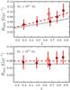Fig. 10

Major (upper panel) and minor (lower panel) merger rate of M_⋆ ≥ 10¹¹ M_⊙ ETGs as a function of redshift. Filled symbols are from the present work, while open ones are from LS11 in VVDS-Deep for red galaxies. Dashed lines are the best fit to the ETGs data, while dotted lines are the fits for the global population.

6. The role of mergers in the evolution of massive ETGs since z = 1

In this section we use the previous merger rates to estimate the number of minor and major mergers per massive (M_⋆ ≥ 10¹¹ M_⊙) ETG since z = 1 (Sect. 6.1) and the impact of mergers in the mass growth (Sect. 6.2) and size evolution (Sect. 6.3) of ETGs in the last ~8 Gyr.

6.1. Number of minor mergers since z = 1

We can obtain the average number of minor mergers per ETG between z₂ and z₁ < z₂ as $N_{mm}^{ET} (z_{1}, z_{2}) = \int_{z_{1}}^{z_{2}} \frac{R_{mm}^{ET} d z}{(1 + z) H_{0} E (z)},$ $\begin{equation} N_{\rm mm}^{\rm ET}(z_1,z_2) = \int_{z_1}^{z_2} \frac{R_{\rm mm}^{\rm ET}\,{\rm d}z}{(1+z)H_0E(z)},\label{numm} \end{equation}$ (23)where $E (z) = \sqrt{Ω_{Λ} + Ω_{m} (1 + z)^{3}}$ $\hbox{$E(z) = \sqrt{\Omega_{\Lambda} + \Omega_{\rm m}(1+z)^3}$}$ in a flat universe. The definition of $N_{MM}^{ET}$ $\hbox{$N_{\rm MM}^{\rm ET}$}$ for major mergers is analogous. Using the merger rates in previous section, we obtain $N_{m}^{ET} = 0.89 \pm 0.14$ $\hbox{$N_{\rm m}^{\rm ET} = 0.89\pm0.14$}$ , with $N_{MM}^{ET} = 0.43 \pm 0.13$ $\hbox{$N_{\rm MM}^{\rm ET} = 0.43\pm0.13$}$ and $N_{mm}^{ET} = 0.46 \pm 0.06$ $\hbox{$N_{\rm mm}^{\rm ET} = 0.46\pm0.06$}$ between z = 1 and z = 0. The number of minor mergers per massive ETGs since z = 1 is therefore similar to the number of major ones. Note that these values and those reported in the following have an additional factor of two uncertainty due to the uncertainty on the merger time scales derived from simulations (Sect. 5).

The number of major mergers per red bright galaxy measured by LS11 is $N_{MM}^{red} = 0.7 \pm 0.2$ $\hbox{$N_{\rm MM}^{\rm red} = 0.7 \pm 0.2$}$ , higher than our measurement, while the number of minor mergers is similar, $N_{mm}^{red} = 0.5 \pm 0.2$ $\hbox{$N_{\rm mm}^{\rm red} = 0.5 \pm 0.2$}$ . The discrepancy in the major merger case can be explained by the evolution of the merger rate in both studies, since LS11 assumed $n_{MM}^{red} = 0$ $\hbox{$n_{\rm MM}^{\rm red} = 0$}$ and we measure $n_{MM}^{ET} = 1.8$ $\hbox{$n_{\rm MM}^{\rm ET} = 1.8$}$ .

On the other hand, LTGs have a significantly lower number of mergers, $N_{m}^{LT} ~ 0.35$ $\hbox{$N_{\rm m}^{\rm LT} \sim 0.35$}$ , with $N_{MM}^{LT} ~ 0.15$ $\hbox{$N_{\rm MM}^{\rm LT} \sim 0.15$}$ and $N_{mm}^{LT} ~ 0.20$ $\hbox{$N_{\rm mm}^{\rm LT} \sim 0.20$}$ . We refer the reader to LS11 for the discussion about the role of major and minor mergers in the evolution of LTGs. In their work, Pozzetti et al. (2010) find that almost all the evolution in the stellar mass function since z ~ 1 is a consequence of the observed star formation (see also Vergani et al. 2008), and estimate that N_m ~ 0.7 mergers since z ~ 1 per log (M_⋆/M_⊙) ~ 10.6 galaxy are needed to explain the remaining evolution. Their result is similar to our direct estimation for the global massive population (ETGs + LTGs), N_m = 0.75 ± 0.14, but they infer N_MM < 0.2. This value is half of ours, N_MM = 0.36 ± 0.13, pointing out that close pair studies are needed to understand accurately the role of major/minor mergers in galaxy evolution.

6.2. Mass assembled through mergers since z = 1

Following LS11, we estimate the mass assembled due to mergers by weighting the number of mergers in the previous section with the average major ( $μ_{MM}$ $\hbox{$\overline{\mu}_{\rm MM}$}$ ) and minor merger ( $μ_{mm}$ $\hbox{$\overline{\mu}_{\rm mm}$}$ ) mass ratio, $δ M_{⋆} (z) \equiv \frac{M_{⋆} (0)}{M_{⋆} (z)} - 1 = μ_{MM} N_{MM}^{ET} (0,z) + μ_{mm} N_{mm}^{ET} (0,z) .$ $\begin{equation} \delta M_{\star}(z) \equiv \frac{M_{\star}(0)}{M_{\star}(z)} - 1 = \overline{\mu}_{\rm MM} N^{\rm ET}_{\rm MM}(0,z) + \overline{\mu}_{\rm mm} N^{\rm ET}_{\rm mm}(0,z).\label{deltamass} \end{equation}$ (24)To obtain the average mass ratios we measured the merger fraction of massive ETGs at 0.2 ≤ z < 0.9 for different values of μ, from μ = 1/2 to 1/10. Then, we fitted to the data a power-law, f_m ( ≥ μ) ∝ μ^s, and used the prescription in LS11 to estimate the average merger mass ratio from the value of the power-law index s. Following those steps we find s = −0.95 for massive ETGs in COSMOS, while the average merger mass ratios are $μ_{MM} = 0.48$ $\hbox{$\overline{\mu}_{\rm MM} = 0.48$}$ and $μ_{mm} = 0.15$ $\hbox{$\overline{\mu}_{\rm mm} = 0.15$}$ , similar to those values reported by LS11. With all previous results we obtain that mergers with μ ≥ 1/10 increase the stellar mass of massive ETGs by δM_⋆ = 28 ± 8% since z = 1. LS11 find δM_⋆(1) = 40 ± 10% for red bright galaxies in VVDS-Deep, consistent with our measurement within errors. We note that they use B-band luminosity as a proxy of stellar mass, so their value is an upper limit due to the lower mass-to-light ratio of blue companions. Bluck et al. (2012) study the major and minor (μ ≥ 1/100) merger fraction of massive galaxies at 1.7 < z < 3 in GNS⁸ (GOODS NICMOS Survey, Conselice et al. 2011). They extrapolate their results to lower redshifts, estimating δM_⋆(1) = 30 ± 25% for μ ≥ 1/10 mergers. Their value is in good agreement with our measurement, but its large uncertainty prevents a quantitative comparison.

The relative contribution of major/minor mergers to our inferred mass growth is 75%/25% because the average major merger is three times more massive than the average minor one, as already pointed out by LS11. In their cosmological model, Hopkins et al. (2010a) predict that the relative contribution of major and minor mergers in the spheroids assembly of log (M_⋆/M_⊙) ~ 11.2 galaxies is ~ 80%/20%, in good agreement with our observational result.

On the other hand, several authors have studied luminosity functions and clustering to constrain the evolution of luminous red galaxies (LRGs) with redshift, finding that LRGs have increased their mass δM_⋆ ~ 30−50% by merging since z = 1 (Brown et al. 2007, 2008; Cool et al. 2008). Their results are similar to our direct estimation, but we must take this agreement with caution. Tal et al. (2012) show that LRGs have a lack of major companions, excluding major mergers as an important growth channel (see also De Propris et al. 2010). Typically LRGs have L ≳ 3L^∗, and a low impact of major mergers in this systems is indeed expected by cosmological models, where the contribution of major mergers in galaxy mass assembly peaks at ~ $M_{⋆}^{*}$ $\hbox{$M_{\star}^{*}$}$ (Khochfar & Silk 2009; Hopkins et al. 2010a; Cattaneo et al. 2011). Thus, even if the values of δM_⋆ are similar for LRGs and our massive galaxies, they could have a different origin. A better approach to estimate indirectly the impact of mergers in mass growth is to study the evolution of massive red galaxies at a fixed number density: because they are red (i.e., they have low star formation), their mass is expected to grow only by merging. Following this approach, van Dokkum et al. (2010) and Brammer et al. (2011) estimate δM_⋆(1) ~ 40% for massive galaxies in the NEWFIRM Medium-Band Survey⁹ (van Dokkum et al. 2009). Their result represents the integral over all possible μ values, so in combination with our δM_⋆(1) ~ 30% for μ ≥ 1/10, this would imply that (i) μ ≥ 1/10 mergers dominates the mass assembly of massive galaxies since z = 1 and (ii) there is room for an extra δM_⋆ ~ 10% growth due to very minor mergers (μ < 1/10).

6.3. Size growth due to mergers since z = 1

Since the first results of Daddi et al. (2005) and Trujillo et al. (2006), several authors have studied in details the size evolution of massive ETGs with cosmic time. It is now well established that ETGs were smaller, on average, than their local counterparts of a given stellar mass by a factor of two at z = 1 and of four at z = 2 (Sect. 1). The size evolution is usually parametrised as $δ r_{e} (z) \equiv \frac{r_{e} (z)}{r_{e} (0)} = (1 + z)^{- α},$ $\begin{equation} \delta r_{\rm e}\,(z) \equiv \frac{r_{\rm e}\,(z)}{r_{\rm e}(0)} = (1 + z)^{-\alpha}, \end{equation}$ (25)where r_e is the effective radius of the galaxy. Despite of all observational efforts, the value of α is still in debate, spanning the range α = 0.9 − 1.5 (see references in Sect. 1), as well as its dependency on stellar mass (massive galaxies evolve faster, Williams et al. 2010, or not, Damjanov et al. 2011). In the following we assume as fiducial α value the value reported by van der Wel et al. (2008) from a combination of several analysis, α = 1.2 (δr_e = 0.43 at z = 1), with an uncertainty of 0.2 (dott-dashed line in Fig. 11).

Two main effects could explain the size evolution of ETGs: the progenitor bias and genuine size growth. The number density of massive (red) galaxies at z = 2 is ~15−30% of that in the local universe (e.g., Arnouts et al. 2007; Pérez-González et al. 2008; Williams et al. 2010; Ilbert et al. 2010), and those ETGs that have reached the red sequence at later times are systematically more extended than those which did it at high redshift. This effect is called the progenitor bias and mimic a size growth (see van der Wel et al. 2009a; Valentinuzzi et al. 2010a,b; Cassata et al. 2011, for further datails). Both van der Wel et al. (2009a) and Saglia et al. (2010) estimate that the progenitor bias of massive ETGs accounts for a factor 1.25 (δr_e = 0.8) of the size evolution since z = 1, and we assume this value in the following.

Regarding size growth, several authors have suggested that compact galaxies at z ~ 2 are the cores of present day massive ellipticals, and that they increase their size by adding stellar mass in the outskirts of the compact high redshift galaxy (Bezanson et al. 2009; Hopkins et al. 2009a; van Dokkum et al. 2010; Weinzirl et al. 2011). The fact that the more compact galaxies at z ~ 0.1 (Trujillo et al. 2009) and z ~ 1 (Martinez-Manso et al. 2011) have similar young ages (~1−2 Gyr), combined with their paucity in the local universe (Trujillo et al. 2009; Taylor et al. 2010; Cassata et al. 2011) also support the size evolution of these systems along cosmic time. Mergers, specially the minor ones, have been proposed to explain this evolution (e.g., Naab et al. 2009; Bezanson et al. 2009; Hopkins et al. 2010b; Weinzirl et al. 2011). Adiabatic expansion due to AGN activity (Fan et al. 2010) or stellar evolution (Damjanov et al. 2009) could also play a role. Thanks to our direct measurements of the minor and major merger rate of massive ETGs, we are able to explore the contribution of mergers to the size growth of these galaxies in the last ~8 Gyr.

Theory and simulations show that equal-mass mergers between two spheroidal galaxies are less effective in increasing the size of ETGs than a major/minor merger with a less dense galaxy, both spiral and spheroidal. In the first case the increase in size is proportional to the accreted mass, $r_{e} \propto M_{⋆}^{β}$ $\hbox{$r_{\rm e} \propto M_{\star}^{\beta}$}$ , with β = 1, while in the second case the index β is higher and spans a wide range, β ~ 1.5−2.5 (e.g., Bezanson et al. 2009; Hopkins et al. 2010b). In our case, we estimate β for a given μ from the relation between the initial (r_e,i) and the final effective radius (r_e,f) of an ETG in a merger process derived by Fan et al. (2010), $\frac{r_{e, f}}{r_{e, i}} = \frac{(1 + μ)^{2}}{1 + μ^{2 - ϵ}} = (1 + μ)^{β},$ $\begin{equation} \frac{r_{\rm e,f}}{r_{\rm e,i}} = \frac{(1 + \mu)^2}{1 + \mu^{2 - \epsilon}} = (1 + \mu)^{\beta},\label{req} \end{equation}$ (26)where ϵ is the slope of the stellar mass vs size relation. In their work, Damjanov et al. (2011) find ϵ = 0.51 for early-type galaxies in the range 0.2 < z < 2 (see also Williams et al. 2010; Newman et al. 2012), similar to the ϵ = 0.56 from Shen et al. (2003) in SDSS¹⁰ (Sloan Digital Sky Survey, Abazajian et al. 2009) or the ϵ ~ 0.5 expected from the Faber-Jackson relation (Faber & Jackson 1976). However, not all the observed mergers are between two early-type galaxies. Using colour as a proxy for the morphology of our companion galaxies, we find that 65% of the mergers are “dry” (red-red), while 35% are “mixed” (red-blue), for both major and minor mergers (Sect. 4.3). In the mixed case we use ϵ = 0.27, a value estimated from the data of Shen et al. (2003) for late-type galaxies in our mass range of interest. Finally, we obtain the β for a given μ as 0.65β_dry + 0.35β_mixed. Using the average mass ratios $μ_{MM}$ $\hbox{$\overline{\mu}_{\rm MM}$}$ and $μ_{mm}$ $\hbox{$\overline{\mu}_{\rm mm}$}$ in Sect. 6.2, we find β_MM = 1.30 for major mergers and β_mm = 1.65 for minor ones.

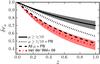Fig. 11

Effective radius normalised to its local value, δr_e, as a function of redshift. The dott-dashed line is the observational evolution from van der Wel et al. (2008), δr_e = (1 + z)^-1.2. The solid line is the evolution due to major and minor mergers (μ ≥ 1/10) expected from our results. The shaded areas in both cases mark the 68% confidence interval. The dotted line is the expected evolution when the progenitor bias (PB) is taken into account. The dashed line is the expected evolution when PB and very minor mergers (μ < 1/10) are included (see text for details).

Following Eq. (24), we trace the mass growth of massive ETGs with redshift for both minor, δM_⋆ ,mm(z), and major mergers, δM_⋆ ,MM(z). Then, we translate these mass growths to a size growth with the previous values of β, $δ r_{e}^{m} (z) = [1 + δ M_{⋆, MM} (z)]^{- β_{MM}} \times [1 + δ M_{⋆, mm} (z)]^{- β_{mm}} \cdot$ $\begin{equation} \delta r_{\rm e}^{\rm m}\,(z) = [1 + \delta M_{\star,{\rm MM}}(z)]^{-\beta_{\rm MM}} \times [1 + \delta M_{\star,{\rm mm}}(z)]^{-\beta_{\rm mm}}\cdot \end{equation}$ (27)Finally, we estimate the contribution of mergers to the total size evolution since z = 1 as $Δ r_{e} = \frac{1 - δ r_{e}^{m} (1)}{1 - δ r_{e} (1)} \cdot$ $\begin{equation} \Delta r_{\rm e} = \frac{1 - \delta r_{\rm e}^{\rm m}(1)}{1 - \delta r_{\rm e}(1)}\cdot \end{equation}$ (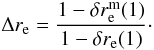28)This model yields a size evolution due to mergers of $δ r_{e}^{m} (1) = 0.70$ $\hbox{$\delta r_{\rm e}^{\rm m}(1) = 0.70$}$ (α = 0.52 ± 0.12, solid line in Fig. 11). This implies that observed major and minor mergers can explain Δr_e ~ 55% of the size evolution in massive ETGs since z ~ 1. In the following, all quoted Δr_e have a typical ~ 15% uncertainty due to the errors in the merger rates and in the observed size evolution.

We take into account the progenitor bias by applying a linear function to the previous size growth due to mergers (dotted line in Fig. 11), $δ r_{e}^{PB} (z) = (1 - 0.2 z) \times δ r_{e}^{m} (z) .$ $\begin{equation} \delta r_{\rm e}^{\rm PB}\,(z) = (1 - 0.2z) \times \delta r_{\rm e}^{\rm m}\,(z). \end{equation}$ (29)We obtain $δ r_{e}^{PB} (1) = 0.56$ $\hbox{$\delta r_{\rm e}^{\rm PB}(1) = 0.56$}$ (α = 0.84 ± 0.12), thus explaining Δr_e ~ 75% of the size evolution with our current observations. We note that this value is similar to the δr_e(1) = 0.63 estimated by the simple model of van der Wel et al. (2009a), which only includes the progenitor bias and a merger prescription from cosmological simulations. The remaining Δr_e ~ 25% of the evolution should be explained by other physical processes (e.g., very minor mergers with μ < 1/10 or adiabatic expansion) or by systematic errors in the measurements (e.g., lower merger time scales or an overestimation of the size evolution). We explore these processes/systematics in the following.

Very minor mergers(μ < 1/10). Cosmological simulations find that μ ≥ 1/10 mergers are not the more common ones, with the merger history of massive galaxies being dominated by μ < 1/10 mergers (Shankar et al. 2010; Jiménez et al. 2011; Oser et al. 2012). However, in this simulations the mass accretion is dominated by μ ≥ 10 events due to the low mass of the very minor companions. As we show in Sect. 6.2, a mass growth of δM_⋆ ~ 10% due to very minor mergers since z = 1 is compatible with the observed mass assembly of massive red galaxies (van Dokkum et al. 2010; Brammer et al. 2011). This translates to N_vm ~ 4 very minor mergers per massive ETG since z ~ 1 (we assumed that very minor mergers have 1/100 ≤ μ < 1/10 and estimated that $μ_{vm} ~ 0.025 = 1 / 40$ $\hbox{$\overline{\mu}_{\rm vm} \sim 0.025 = 1/40$}$ following the prescriptions in Sect. 6.2). Note that we can increase arbitrarily the number of very minor mergers by lowering $μ_{vm}$ $\hbox{$\overline{\mu}_{\rm vm}$}$ , but not their contribution to the mass growth, which is fixed. We checked that the conclusions in this section are independent of $μ_{vm}$ $\hbox{$\overline{\mu}_{\rm vm}$}$ . We estimate β_vm = 1.85 for very minor mergers, thus obtaining an extra size growth of Δr_e ~ 20% due to mergers, $δ r_{e}^{m} (1) = 0.58$ $\hbox{$\delta r_{\rm e}^{\rm m}(1) = 0.58$}$ and α = 0.78 ± 0.12 when all μ values are taken into account. Hence, mergers since z ~ 1 may explain Δr_e ~ 75% of the observed size evolution, while Δr_e ~ 95%, with $δ r_{e}^{PB} (1) = 0.47$ $\hbox{$\delta r_{\rm e}^{\rm PB}(1) = 0.47$}$ and α = 1.1, when the progenitor bias is taken into account (dashed line in Fig. 11). In this picture, nearly half of the evolution due to mergers is related to minor (μ < 1/4) events. This result reinforces our conclusion that mergers are the main contributors to the size evolution of massive ETGs since z = 1, but observational estimations of the very minor merger rate (μ < 1/10) are needed to constraint their role. As a first attempt, Mármol-Queraltó et al. (2012) find that the merger fraction of massive galaxies at z ≲ 1 for μ ≥ 1/100 satellites is two times that of μ ≥ 1/10 satellites. That suggests N_vm ~ 1, and an additional contribution for even smaller satellites (μ < 1/100) could be possible.
Adiabatic expansion. This will occur in a relaxed system that is losing mass. As mass is lost the potential becomes shallower, so the system expands into a new stable equilibrium. The amount that a system expands depends on both the ejected mass (M_⋆ ,eject) and on the time scale of the process (T_eject). Fan et al. (2008, 2010) suggest adiabatic expansion due to quasar activity and/or supernova winds as an alternative process to explain the size growth of massive early-types, specially at z ≳ 1. These processes occur on very short time scales after the formation of the spheroid (T_eject ≲ 0.5 Gyr, Ragone-Figueroa & Granato 2011), so we expect those galaxies with stellar populations older than ~ 1 Gyr to be already located in the local stellar mass-size relation. This is not supported by observations, in which galaxies older than ≳ 3 Gyr at z ~ 1 are still smaller than the local ones (see Trujillo et al. 2011, for details). Interestingly, minor mergers with gas-rich satellites (~35% of our observed mergers) could trigger recent star formation and AGN activity in massive early types (e.g., Kaviraj et al. 2009; Fernández-Ontiveros et al. 2011), therefore favouring some degree of adiabatic expansion and adding an extra size growth to the merging process. Devoted N-body simulations are needed to explore this topic in details. It is also to be noted that the mass loss due to stellar winds from the passive evolution of stellar populations in a galaxy may lead to adiabatic expansion (Damjanov et al. 2009). Ragone-Figueroa & Granato (2011) show that a typical massive galaxy is able to eject enough mass due to galactic winds to increase its size by a factor of 1.2 in ~ 8 Gyr. This result assumes that the potential of the galaxy is not able to retain any of the ejected mass, so this could indicate that at most Δr_e ~ 20% of the size evolution since z = 1 could be explained by stellar winds.
Overestimation of the size evolution. Results from Martinez-Manso et al. (2011) suggest that the photometric stellar masses of Trujillo et al. (2007) are an order of magnitude higher than those estimated from velocity dispersion measurements. This does not erase the size evolution, but makes it smaller (massive galaxies are more extended than less massive ones at a given redshift, e.g., Damjanov et al. 2011). Taking dynamical masses (M_dym) as a reference instead of photometric ones, van der Wel et al. (2008) find α = 0.98 ± 0.11, smaller than the α = 1.20 found by the same authors from photometric studies. The same trend is found by Saglia et al. (2010) from the ESO Distant Cluster Survey¹¹ (EDisCS; White et al. 2005) galaxies: α ~ 0.65 from dynamical masses vs α ~ 0.85 from stellar masses after the progenitor bias is accounted for. Finally, Newman et al. (2010) find α ~ 0.75 for M_dym ≥ 10¹¹ M_⊙ galaxies. Assuming these smaller α values from dynamical masses, major and minor mergers account for Δr_e ~ 65% of the size evolution, and all the evolution is explained when the progenitor bias and very minor mergers are taken into account. It is also possible that the extended, low-surface brightness envelopes of high-z galaxies were missed and their r_e were correspondingly underestimated. However, deep observations in the near infrared (optical rest-frame) from space (Szomoru et al. 2010; Cassata et al. 2010; Weinzirl et al. 2011) and from ground-based facilities with adaptive optics (Carrasco et al. 2010) confirm the compactness of 1 ≲ z ≲ 3 massive galaxies. On the other hand, also higher values of α than our fiducial value α = 1.2 ± 0.2 are present in the literature. For example, Buitrago et al. (2008) find α = 1.51 ± 0.04 at z < 2, while Damjanov et al. (2011) find α = 1.62 ± 0.34. Assuming α = 1.5, μ ≥ 1/10 mergers would explain Δr_e ~ 45% of the size evolution, while the addition of very minor mergers would increase the role of mergers up to Δr_e ~ 65%. In that case, the contribution of other processes would increases to Δr_e ~ 20%. Thus, even if the size evolution is faster than our fiducial α value, mergers would be still the dominant mechanism.
Merger time scale. The main uncertainty in our merger rates is the assumed merger time scale, which typically has a factor of two uncertainty in their normalisation (e.g., Hopkins et al. 2010c). The T_MM from Kitzbichler & White (2008) are typically longer than others in the literature (e.g., Patton & Atfield 2008; Lin et al. 2010) or similar to those from N-body/hydrodynamical simulations (Lotz et al. 2010b,a). Thus, we expect, if anything, a shorter T_MM, which implies a larger role of mergers in size evolution (i.e., higher merger rates and number of mergers since z ~ 1). In fact, a shorter T_MM by a factor of 1.5 is enough to explain the observed mass growth and size evolution without the contribution of very minor mergers.
Uncertainties in β. Equation (26), which we used to derive the values of β in our model, assumes parabolic orbits and dissipationless (gas-free) mergers. About the first assumption, Khochfar & Burkert (2006) and Wetzel & White (2010) show that most dark matter halos in cosmological simulations merge on parabolic orbits. On the other hand, we find that ~ 65% of our mergers are dry, but the other ~ 35% are mixed and an extra dissipative component is present (Sect 4.3). In these cases simulations suggest that β should be higher than derived from Eq. (26), even reaching β ~ 2.5 (Hopkins et al. 2010b). This does not change our conclusions because it translates to a higher size evolution due to mergers. In addition, Oser et al. (2012) show that the size growth expected from Eq. (26) is in nice agreement with the growth measured in hydrodynamical simulations settled in a cosmological contest.

In summary, our results suggest that merging is the main contributor to the size evolution of massive ETGs, accounting for Δr_e ~ 50 − 75% of the observed evolution since z ~ 1. Nearly half of the evolution due to mergers is related to minor (μ < 1/4) events.

6.3.1. Additional constraints from velocity dispersion evolution

In addition to their mass and size, the velocity dispersion (σ_⋆) of ETGs evolves with redshift as δσ_⋆(z) = σ_⋆(z)/σ_⋆(0) = (1 + z)^a. We assume a = 0.4 ± 0.1 in the following (δσ_⋆ = 1.32 at z = 1, Cenarro & Trujillo 2009; Cappellari et al. 2009; Saglia et al. 2010; van de Sande et al. 2011). When we apply our simple model using the prescriptions of Fan et al. (2010) for the evolution of σ_⋆ in merger events, μ ≥ 1/10 mergers are only able to explain 15% of the observed evolution, $δ σ_{⋆}^{m} (1) = 1.05$ $\hbox{$\delta \sigma_{\star}^{\rm m}(1) = 1.05$}$ . Hopkins et al. (2009b) propose another prescription to trace the evolution in σ_⋆ from the evolution in size that takes into account the dark matter component of the galaxy, $δ σ_{⋆}^{m} (z) = \sqrt{\frac{γ + 1 / δ r_{e}^{m} (z)}{1 + γ}},$ $\begin{equation} \delta \sigma_{\star}^{\rm m}(z) = \sqrt{\frac{\gamma + 1/\delta r_{\rm e}^{\rm m}(z)}{1 + \gamma}}, \end{equation}$ (30)where γ ~ 1 for M_⋆ ~ 10¹¹ M_⊙ galaxies. Using this prescription, the evolution of σ_⋆ is faster, but we still explain only ~ 35% of the observed evolution, $δ σ_{⋆}^{m} (1) = 1.10$ $\hbox{$\delta \sigma_{\star}^{\rm m}(1) = 1.10$}$ (solid line in Fig. 12). The addition of very minor mergers increase the contribution to ~ 50%, $δ σ_{⋆}^{m} (1) = 1.16$ $\hbox{$\delta \sigma_{\star}^{\rm m}(1) = 1.16$}$ (dotted line in Fig. 12). However, a small change of σ_⋆ due to mergers is consistent with the picture from Bernardi et al. (2011). They study in details the colour − M_⋆ and colour − σ_⋆ relation of ETGs in SDSS, finding that M_⋆ ~ 2 × 10¹¹ M_⊙ is a transition mass (M_tran) for which the curvature of the colour − M_⋆ relation change, while no deviation is present in the colour − σ_⋆ relation. These authors claim that (dry) mergers are the main process in the evolution of those ETGs with $M_{⋆} ≳ M_{tran} ~ M_{⋆}^{*}$ $\hbox{$M_{\star} \gtrsim M_{\rm tran} \sim M_{\star}^*$}$ (see also van der Wel et al. 2009b; López-Sanjuan et al. 2010b; Oesch et al. 2010; Eliche-Moral et al. 2010; Méndez-Abreu et al. 2012, for a similar conclusion), as our results also suggest.

One missing ingredient in the model described in this section is the progenitor bias: new early-types which appeared since z ~ 1 are not only more extended that previous ones, but also have a lower velocity dispersion (van der Wel et al. 2009a). Thus, the progenitor bias also mimic a decrease of σ_⋆ with cosmic time. The results of Saglia et al. (2010) suggest that a factor of 1.1 in the σ_⋆ evolution is due to the progenitor bias. Applying this extra evolution as a factor 1 + 0.1z to that from mergers (very minor ones included), we are able to explain 90% of the increase in velocity dispersion, $δ σ_{⋆}^{PB} (1) = 1.28$ $\hbox{$\delta \sigma_{\star}^{\rm PB}(1) = 1.28$}$ (dashed line in Fig. 12). Including this, our model is compatible with the observed evolution and suggests that mergers and the progenitor bias have a similar contribution to σ_⋆ evolution, somewhat different from the dominant role of mergers in size evolution.

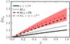Fig. 12

Velocity dispersion normalised to its local value, δσ_⋆, as a function of redshift. The dott-dashed line is the observed evolution, δσ_⋆ = (1 + z)^0.4. The shaded area marks the 68% confidence interval. The solid line is the evolution due to major and minor mergers (μ ≥ 1/10) expected from our results. The dotted line is the expected evolution when very minor mergers (μ < 1/10) are taken into account. The dashed line is the expected evolution when very minor mergers and the progenitor bias (PB) are included (see text for details).

6.3.2. Additional constraints from Sérsic index evolution

Other structural parameters of ETGs, as the Sérsic index n_s (Sérsic 1968), also evolve with redshift. Depending on the value of n_s, galaxies can be described as disc-like with a n_s = 1 exponential profile or bulge-like with higher n_s values, where ellipticals are expected to have n_s = 4 profiles. We refer to the change in the Sérsic index with redshift as $Δ n_{s} (z) = n_{s} (0) - n_{s} (z),$ $\begin{equation} \Delta n_{\rm s}(z) = n_{\rm s}(0) - n_{\rm s}(z), \end{equation}$ (31)where n_s(z) is the Sérsic index at redshift z. Several studies find that the Sérsic index of the global massive population decreases with redshift (e.g., van Dokkum et al. 2010; Weinzirl et al. 2011; Buitrago et al. 2011), evolving from n_s(1) ~ 3 to n_s(0) ~ 6, Δn_s(1) ~ 3. Focusing on massive ETGs, the study of Buitrago et al. (2011) find an evolution in n_s consistent with Δn_s(z) = 1.4z up to z ~ 2.5, and we take this evolution as a reference.

We used the theoretical results in Hopkins et al. (2010b) to estimate the change in the Sérsic index of ETGs since z ~ 1 due to mergers. We took their results for minor mergers/late accretion as representative, so we can roughly estimate Δn_s(z) for a given increase in effective radius (their Fig. 3). From the values of $δ r_{e}^{m}$ $\hbox{$\delta r_{\rm e}^{\rm m}$}$ estimated in Sect. 6.3, we expect Δn_s(1) ~ 1−2. This evolution is in agreement with the Δn_s(1) = 1.4 measured by Buitrago et al. (2011) for massive ETGs. We conclude that the observed merging activity is also consistent with the observed evolution in the Sérsic index of massive ETGs, supporting the dominant role of mergers in the evolution of these systems since z ~ 1.

6.3.3. Additional constraints from scaling relations

Nipoti et al. (2009) point out that the tightness of the local scaling laws of ETGs posses an important limit to the growth of these systems by (dry) merging (see also Ciotti et al. 2007; Nair et al. 2011). Using these local scaling laws, they conclude that typical present-day massive ETGs could not have assembled more than ~ 45% of their present stellar mass and grew more than a factor ~ 1.9 in size via merging. Even if uncertain, we can extrapolate our observed trends up to z ~ 2 and compare the inferred mass and size growths with these upper limits provided by Nipoti et al. (2009). We obtain a mass growth by merging (including very minor mergers) of δM_⋆ ~ 60% since z = 2, which implies that δM_⋆(2)M_⋆(2)/M_⋆(0) ~ 40% of the total mass at z = 0 was assembled by merging since z = 2. The size grows by a factor of ~ 2 due to this merging in the same cosmic time lapse. Therefore, merging seems compatible with the upper limits in mass assembly and size growth imposed by the tightness of the local scaling laws, although a more complex model is needed to fully explore how these laws evolve due to our observed merger history.

6.3.4. Comparison with previous studies

In a previous work, Trujillo et al. (2011) use a similar model than ours to estimate the number of mergers needed since z ~ 1 to explain size evolution if merging is the only process involved. They conclude that N_m = 5.0 ± 1.64 mergers with μ = 1/3 are needed. This number of mergers is higher than our direct measurement by a factor of five, N_m = 0.89 ± 0.14 (our average merger with μ ≥ 1/10 has $μ ~ 1 / 3$ $\hbox{$\overline{\mu} \sim 1/3$}$ ). If we take into account our estimated very minor mergers, our numbers are N_m ~ 5 and $μ ~ 1 / 10$ $\hbox{$\overline{\mu} \sim 1/10$}$ . For this value of μ they infer N_m = 11.20 ± 3.66, still higher than our estimation. The model of Trujillo et al. (2011) also estimates the mass growth due to mergers since z ~ 1, which is a factor of 3 − 5, also higher than any observational estimation or constraint (a factor of ~1.4, Sect. 6.2).

Newman et al. (2012) study the size evolution of red galaxies in the CANDELS¹² (Cosmic Assembly Near-infrared Deep Extragalactic Legacy Survey, Grogin et al. 2011; Koekemoer et al. 2011) survey and the role of mergers with μ ≥ 1/10 in this size growth at 0.4 < z < 2. Applying a similar model than ours to translate their observed total merger fraction to a size growth, they conclude that merging can reasonably account for the size evolution observed at z ≲ 1 after the progenitor bias is taking into account, while at z ≳ 1 mergers are not common enough. Despite the fact that they only have one merger fraction data point at 0.4 < z < 1 (Fig. 8), their conclusion is consistent with our more detailed study at z ≲ 1.

6.3.5. Expectations from cosmological models

Several theoretical efforts have been conducted to explain the size evolution of ETGs. In this section we compare the predicted size evolution from cosmological models with our best model, which suggests that Δr_e ~ 75% of the evolution in size is due to mergers, Δr_e ~ 20% to the progenitor bias and Δr_e ~ 5% to other processes (e.g., adiabatic expansion).

The model of Hopkins et al. (2010b) predicts that, since z = 2, un-equal mass mergers explain Δr_e ~ 60% of the observed size evolution, in agreement with our result. However, these authors only track the evolution of compact galaxies since z = 2 and do not take into account the possible contribution of the progenitor bias, but argue that it should impact their predictions. In fact, they predict that ~ 45% of the size evolution since z = 1 is due to un-equal mass mergers, another ~ 45% is accounted for by systematics in size measurements and the extra ~ 10% is due to adiabatic expansion, probably reflecting their biased population.

The model of Shankar et al. (2012) predicts δr_e ~ 0.7 for massive galaxies, in agreement with our observational derivation due only to mergers (see also Khochfar & Silk 2006). Interestingly, the evolution increases to δr_e ~ 0.5 when individual galaxies are tracked along their evolution without any stellar mass selection. They predict that ~ 40% of the mass accreted by merging in massive galaxies is due to major mergers with μ ≥ 1/3. Our best model implies that ~ 47% of mass and size growth is due to major mergers with μ ≥ 1/3. The qualitative agreement between both works is remarkable.

On the other hand, Oser et al. (2012) find α = 1.12 (α = 1.44 for passive galaxies) and a ~ 0.4 by re-simulating with high resolution a set of 40 galaxies with M_⋆ ≥ 6.3 × 10¹⁰ M_⊙ in a cosmological context. They find that the number-averaged merger has $μ = 1 / 16$ $\hbox{$\overline{\mu} = 1/16$}$ , while the mass-averaged merger has $μ_{⋆} = 1 / 5$ $\hbox{$\overline{\mu}_{\star} = 1/5$}$ . From our model we estimate $μ_{⋆} = 1 / 3$ $\hbox{$\overline{\mu}_{\star} = 1/3$}$ and $μ = 1 / 13$ $\hbox{$\overline{\mu} = 1/13$}$ . We check that $μ_{⋆}$ $\hbox{$\overline{\mu}_{\star}$}$ is independent of the assumed number of very minor mergers N_vm, while we can vary $μ$ $\hbox{$\overline{\mu}$}$ arbitrarily by changing N_vm. Thus, only the comparison with $μ_{⋆}$ $\hbox{$\overline{\mu}_{\star}$}$ is representative. The predicted value is lower than our measurement, but they find a higher role of major mergers at M_⋆ ~ 10^11.1 M_⊙ (see also Khochfar & Silk 2009; Hopkins et al. 2010a; Cattaneo et al. 2011), with $μ_{⋆} ~ 1 / 3$ $\hbox{$\overline{\mu}_{\star} \sim 1/3$}$ and a big dispersion due to the low statistics (see their Fig. 6). Future simulations with higher number of galaxies are needed to explore in more details this issue.

In summary, our result that merging is the main process involved in size evolution mostly agrees with simulations, but more observational and theoretical studies are needed to understand the remaining discrepancies.

7. Conclusions

We have measured the minor and major merger fraction and rate of massive (M_⋆ ≥ 10¹¹ M_⊙) galaxies from close pairs in the COSMOS field, and explored the role of mergers in the mass growth and size evolution of massive ETGs since z ~ 1.

We find that the merger fraction and rate of massive galaxies evolves as a power-law (1 + z)ⁿ, with no or only small evolution of the minor merger rate, n_mm ~ 0, in contrast with the increase of the major merger rate, n_MM = 1.4. The total (major + minor) merger rate evolves slower than the major one, with n_m = 0.6. When splitting galaxies according to their HST/ACS morphology, the minor merger fraction for ETGs is higher by a factor of three than that for LTGs, and both are nearly constant with redshift. The fraction of major mergers for LTGs evolves faster ( $n_{MM}^{LT} ~ 4$ $\hbox{$n_{\rm MM}^{\rm LT} \sim 4$}$ ) than for ETGs ( $n_{MM}^{ET} = 1.8$ $\hbox{$n_{\rm MM}^{\rm ET} = 1.8$}$ ). We also find that when we repeat our study with a constant number-density sample, comprising ETGs with log (M_⋆/M_⊙) ≥ 11.15 − 0.15z, the evolution of the major merger fraction is faster ( $n_{MM}^{ET} = 2.5$ $\hbox{$n_{\rm MM}^{\rm ET} = 2.5$}$ ), whilst the minor merger fraction and other derived quantities remain the same. Therefore, we conclude that the selection of the massive ETGs sample has limited impact in our results below.

Our results imply that massive ETGs have undergone 0.89 mergers (0.43 major and 0.46 minor) since z ~ 1, leading to a mass growth of ~30% (75%/25% due to major/minor mergers). We use a simple model to translate the estimated mass growth due to mergers into an effective radius growth. With this model we find that μ ≥ 1/10 mergers can explain ~55% of the observed size evolution since z ~ 1. We infer that another ~20% is due to the progenitor bias (the new ETGs appeared since z = 1 are more extended than their high-z counterparts) and we estimate that very minor mergers (μ < 1/10) could contribute with an additional ~20%. The remaining ~5% could come from adiabatic expansion due to stellar winds or from observational effects. In addition, our picture also reproduces the mass growth and the velocity dispersion evolution of these massive ETGs galaxies since z ~ 1.

We conclude from these results, and after exploring all the possible uncertainties in our model, that merging is the main contributor to the size evolution of massive ETGs at z ≲ 1, accounting for ~50−75% of that evolution in the last 8 Gyr. Nearly half of the evolution due to mergers is related to minor (μ < 1/4) events.

Studies in larger sky areas are needed to improve the statistics, especially at lower redshifts when the cosmological volume probed is still the main source of uncertainty. We point out that a local measurement of the minor merger fraction and rate is needed to better constrain its evolution with redshift. Understanding the dependency of the minor merger rate on stellar mass, as well as extending observations to the very minor merger regime (μ ≤ 1/10) will be important to further improve this picture. In addition, extending the observational work at z > 1, when the massive red sequence seems to emerge, will be necessary to probe the early epochs of mass assembly.

¹

http://cosmos.astro.caltech.edu/

²

http://www.astro.phys.ethz.ch/zCOSMOS/

³

http://cesam.oamp.fr/vvdsproject/vvds.htm

⁴

http://www.stsci.edu/science/goods/

⁵

http://cfht.hawaii.edu/Science/CFHLS/

⁶

http://www.mpia-hd.mpg.de/GEMS/gems.htm

⁷

http://aegis.ucolick.org/

⁸

http://www.nottingham.ac.uk/astronomy/gns/

⁹

http://www.astro.yale.edu/nmbs/Overview.html

¹⁰

http://www.sdss.org/

¹¹

http://www.mpa-garching.mpg.de/galform/ediscs/index.shtml

¹²

http://candels.ucolick.org/About.html

Acknowledgments

We dedicate this paper to the memory of our six IAC colleagues and friends who met with a fatal accident in Piedra de los Cochinos, Tenerife, in February 2007, with a special thanks to Maurizio Panniello, whose teachings of python were so important for this paper. We thank the comments and suggestions of the anonymous referee. We also thank Ignacio Trujillo, Fernando Buitrago, Carmen Eliche-Moral, Paolo Cassata, Jairo Méndez-Abreu, David Patton, Sara Ellison, Trevor Mendel, and Jorge Moreno for useful discussions. This work is supported by funding from ANR-07-BLAN-0228 and ERC-2010-AdG-268107-EARLY.

References

Abazajian, K. N., Adelman-McCarthy, J. K., Agüeros, M. A., et al. 2009, ApJS, 182, 543 [NASA ADS] [CrossRef] [Google Scholar]
Arnouts, S., Walcher, C. J., Le Fèvre, O., et al. 2007, A&A, 476, 137 [NASA ADS] [CrossRef] [EDP Sciences] [Google Scholar]
Baldry, I. K., Glazebrook, K., Brinkmann, J., et al. 2004, ApJ, 600, 681 [NASA ADS] [CrossRef] [Google Scholar]
Barro, G., Pérez-González, P. G., Gallego, J., et al. 2011, ApJS, 193, 30 [NASA ADS] [CrossRef] [Google Scholar]
Bell, E. F., McIntosh, D. H., Katz, N., & Weinberg, M. D. 2003, ApJS, 149, 289 [NASA ADS] [CrossRef] [Google Scholar]
Bell, E. F., Phleps, S., Somerville, R. S., et al. 2006, ApJ, 652, 270 [NASA ADS] [CrossRef] [Google Scholar]
Bernardi, M., Roche, N., Shankar, F., & Sheth, R. K. 2011, MNRAS, 412, 684 [Google Scholar]
Bezanson, R., van Dokkum, P. G., Tal, T., et al. 2009, ApJ, 697, 1290 [NASA ADS] [CrossRef] [Google Scholar]
Bluck, A. F. L., Conselice, C. J., Bouwens, R. J., et al. 2009, MNRAS, 394, L51 [NASA ADS] [CrossRef] [Google Scholar]
Bluck, A. F. L., Conselice, C. J., Buitrago, F., et al. 2012, ApJ, 747, 34 [NASA ADS] [CrossRef] [Google Scholar]
Brammer, G. B., Whitaker, K. E., van Dokkum, P. G., et al. 2011, ApJ, 739, 24 [NASA ADS] [CrossRef] [Google Scholar]
Bridge, C. R., Carlberg, R. G., & Sullivan, M. 2010, ApJ, 709, 1067 [NASA ADS] [CrossRef] [Google Scholar]
Brown, M. J. I., Dey, A., Jannuzi, B. T., et al. 2007, ApJ, 654, 858 [NASA ADS] [CrossRef] [Google Scholar]
Brown, M. J. I., Zheng, Z., White, M., et al. 2008, ApJ, 682, 937 [NASA ADS] [CrossRef] [Google Scholar]
Bruzual, G., & Charlot, S. 2003, MNRAS, 344, 1000 [NASA ADS] [CrossRef] [Google Scholar]
Buitrago, F., Trujillo, I., Conselice, C. J., et al. 2008, ApJ, 687, L61 [NASA ADS] [CrossRef] [Google Scholar]
Buitrago, F., Trujillo, I., Conselice, C. J., & Haeussler, B. 2011, MNRAS, submitted [arXiv:1111.6993] [Google Scholar]
Bundy, K., Ellis, R. S., Conselice, C. J., et al. 2006, ApJ, 651, 120 [NASA ADS] [CrossRef] [Google Scholar]
Bundy, K., Fukugita, M., Ellis, R. S., et al. 2009, ApJ, 697, 1369 [NASA ADS] [CrossRef] [Google Scholar]
Calzetti, D., Armus, L., Bohlin, R. C., et al. 2000, ApJ, 533, 682 [NASA ADS] [CrossRef] [Google Scholar]
Cameron, E. 2011, PASA, 28, 128 [NASA ADS] [CrossRef] [Google Scholar]
Capak, P., Aussel, H., Ajiki, M., et al. 2007, ApJS, 172, 99 [NASA ADS] [CrossRef] [Google Scholar]
Cappellari, M., di Serego Alighieri, S., Cimatti, A., et al. 2009, ApJ, 704, L34 [NASA ADS] [CrossRef] [Google Scholar]
Carrasco, E. R., Conselice, C. J., & Trujillo, I. 2010, MNRAS, 405, 2253 [NASA ADS] [Google Scholar]
Cassata, P., Giavalisco, M., Guo, Y., et al. 2010, ApJ, 714, L79 [NASA ADS] [CrossRef] [Google Scholar]
Cassata, P., Giavalisco, M., Guo, Y., et al. 2011, ApJ, 743, 96 [NASA ADS] [CrossRef] [Google Scholar]
Cattaneo, A., Mamon, G. A., Warnick, K., & Knebe, A. 2011, A&A, 533, A5 [NASA ADS] [CrossRef] [EDP Sciences] [Google Scholar]
Cenarro, A. J., & Trujillo, I. 2009, ApJ, 696, L43 [NASA ADS] [CrossRef] [Google Scholar]
Chabrier, G. 2003, PASP, 115, 763 [NASA ADS] [CrossRef] [Google Scholar]
Chou, R. C. Y., Bridge, C. R., & Abraham, R. G. 2011, AJ, 141, 87 [NASA ADS] [CrossRef] [Google Scholar]
Ciotti, L., Lanzoni, B., & Volonteri, M. 2007, ApJ, 658, 65 [NASA ADS] [CrossRef] [Google Scholar]
Conselice, C. J., Bundy, K., Trujillo, I., et al. 2007, MNRAS, 381, 962 [NASA ADS] [CrossRef] [Google Scholar]
Conselice, C. J., Bluck, A. F. L., Ravindranath, S., et al. 2011, MNRAS, 417, 2770 [NASA ADS] [CrossRef] [Google Scholar]
Cool, R. J., Eisenstein, D. J., Fan, X., et al. 2008, ApJ, 682, 919 [NASA ADS] [CrossRef] [Google Scholar]
Coupon, J., Ilbert, O., Kilbinger, M., et al. 2009, A&A, 500, 981 [NASA ADS] [CrossRef] [EDP Sciences] [Google Scholar]
Daddi, E., Renzini, A., Pirzkal, N., et al. 2005, ApJ, 626, 680 [NASA ADS] [CrossRef] [Google Scholar]
Damjanov, I., McCarthy, P. J., Abraham, R. G., et al. 2009, ApJ, 695, 101 [NASA ADS] [CrossRef] [Google Scholar]
Damjanov, I., Abraham, R. G., Glazebrook, K., et al. 2011, ApJ, 739, L44 [NASA ADS] [CrossRef] [Google Scholar]
Davis, M., Guhathakurta, P., Konidaris, N. P., et al. 2007, ApJ, 660, L1 [NASA ADS] [CrossRef] [Google Scholar]
De Propris, R., Driver, S. P., Colless, M., et al. 2010, AJ, 139, 794 [NASA ADS] [CrossRef] [Google Scholar]
de Ravel, L., Le Fèvre, O., Tresse, L., et al. 2009, A&A, 498, 379 [NASA ADS] [CrossRef] [EDP Sciences] [Google Scholar]
de Ravel, L., Kampczyk, P., Le Fèvre, O., et al. 2011, A&A, submitted [arXiv:1104.5470] [Google Scholar]
Desai, V., Dey, A., Cohen, E., Le Floc’h, E., & Soifer, B. T. 2011, ApJ, 730, 130 [NASA ADS] [CrossRef] [Google Scholar]
Drory, N., Bundy, K., Leauthaud, A., et al. 2009, ApJ, 707, 1595 [NASA ADS] [CrossRef] [Google Scholar]
Efron, B. 1982, CBMS-NSF Regional Conf. Ser. in App. Math. [Google Scholar]
Eliche-Moral, M. C., Prieto, M., Gallego, J., et al. 2010, A&A, 519, A55 [NASA ADS] [CrossRef] [EDP Sciences] [Google Scholar]
Faber, S. M., & Jackson, R. E. 1976, ApJ, 204, 668 [NASA ADS] [CrossRef] [Google Scholar]
Fan, L., Lapi, A., De Zotti, G., & Danese, L. 2008, ApJ, 689, L101 [NASA ADS] [CrossRef] [Google Scholar]
Fan, L., Lapi, A., Bressan, A., et al. 2010, ApJ, 718, 1460 [NASA ADS] [CrossRef] [Google Scholar]
Feldmann, R., Carollo, C. M., Mayer, L., et al. 2010, ApJ, 709, 218 [NASA ADS] [CrossRef] [Google Scholar]
Fernández-Ontiveros, J. A., López-Sanjuan, C., Montes, M., Prieto, M. A., & Acosta-Pulido, J. A. 2011, MNRAS, 411, L21 [NASA ADS] [Google Scholar]
Fontana, A., Pozzetti, L., Donnarumma, I., et al. 2004, A&A, 424, 23 [NASA ADS] [CrossRef] [EDP Sciences] [Google Scholar]
Fontana, A., Salimbeni, S., Grazian, A., et al. 2006, A&A, 459, 745 [NASA ADS] [CrossRef] [EDP Sciences] [Google Scholar]
George, M. R., Leauthaud, A., Bundy, K., et al. 2011, ApJ, 742, 125 [NASA ADS] [CrossRef] [Google Scholar]
Giavalisco, M., Ferguson, H. C., Koekemoer, A. M., et al. 2004, ApJ, 600, L93 [NASA ADS] [CrossRef] [Google Scholar]
Grogin, N. A., Kocevski, D. D., Faber, S. M., et al. 2011, ApJS, 197, 35 [NASA ADS] [CrossRef] [Google Scholar]
Hernández-Toledo, H. M., Avila-Reese, V., Conselice, C. J., & Puerari, I. 2005, AJ, 129, 682 [NASA ADS] [CrossRef] [Google Scholar]
Hernández-Toledo, H. M., Avila-Reese, V., Salazar-Contreras, J. R., & Conselice, C. J. 2006, AJ, 132, 71 [NASA ADS] [CrossRef] [Google Scholar]
Hopkins, P. F., Bundy, K., Murray, N., et al. 2009a, MNRAS, 398, 898 [NASA ADS] [CrossRef] [Google Scholar]
Hopkins, P. F., Hernquist, L., Cox, T. J., Keres, D., & Wuyts, S. 2009b, ApJ, 691, 1424 [NASA ADS] [CrossRef] [Google Scholar]
Hopkins, P. F., Bundy, K., Croton, D., et al. 2010a, ApJ, 715, 202 [NASA ADS] [CrossRef] [Google Scholar]
Hopkins, P. F., Bundy, K., Hernquist, L., Wuyts, S., & Cox, T. J. 2010b, MNRAS, 401, 1099 [NASA ADS] [CrossRef] [Google Scholar]
Hopkins, P. F., Croton, D., Bundy, K., et al. 2010c, ApJ, 724, 915 [NASA ADS] [CrossRef] [Google Scholar]
Ilbert, O., Capak, P., Salvato, M., et al. 2009, ApJ, 690, 1236 [NASA ADS] [CrossRef] [Google Scholar]
Ilbert, O., Salvato, M., Le Floc’h, E., et al. 2010, ApJ, 709, 644 [NASA ADS] [CrossRef] [Google Scholar]
Jiménez, N., Cora, S. A., Bassino, L. P., Tecce, T. E., & Smith Castelli, A. V. 2011, MNRAS, 417, 785 [NASA ADS] [CrossRef] [Google Scholar]
Jogee, S., Miller, S. H., Penner, K., et al. 2009, ApJ, 697, 1971 [NASA ADS] [CrossRef] [Google Scholar]
Kampczyk, P., Lilly, S. J., de Ravel, L., et al. 2011, ApJ, submitted [arXiv:1112.4842] [Google Scholar]
Kartaltepe, J. S., Sanders, D. B., Scoville, N. Z., et al. 2007, ApJS, 172, 320 [NASA ADS] [CrossRef] [Google Scholar]
Kaviraj, S., Schawinski, K., Devriendt, J. E. G., et al. 2007, ApJS, 173, 619 [NASA ADS] [CrossRef] [Google Scholar]
Kaviraj, S., Khochfar, S., Schawinski, K., et al. 2008, MNRAS, 388, 67 [NASA ADS] [CrossRef] [Google Scholar]
Kaviraj, S., Peirani, S., Khochfar, S., Silk, J., & Kay, S. 2009, MNRAS, 394, 1713 [NASA ADS] [CrossRef] [Google Scholar]
Kaviraj, S., Tan, K.-M., Ellis, R. S., & Silk, J. 2011, MNRAS, 411, 2148 [NASA ADS] [CrossRef] [Google Scholar]
Khochfar, S., & Burkert, A. 2006, A&A, 445, 403 [NASA ADS] [CrossRef] [EDP Sciences] [Google Scholar]
Khochfar, S., & Silk, J. 2006, ApJ, 648, L21 [NASA ADS] [CrossRef] [Google Scholar]
Khochfar, S., & Silk, J. 2009, MNRAS, 397, 506 [NASA ADS] [CrossRef] [Google Scholar]
Kitzbichler, M. G., & White, S. D. M. 2008, MNRAS, 1300 [Google Scholar]
Koekemoer, A. M., Aussel, H., Calzetti, D., et al. 2007, ApJS, 172, 196 [NASA ADS] [CrossRef] [Google Scholar]
Koekemoer, A. M., Faber, S. M., Ferguson, H. C., et al. 2011, ApJS, 197, 36 [NASA ADS] [CrossRef] [Google Scholar]
Kovač, K., Lilly, S. J., Cucciati, O., et al. 2010, ApJ, 708, 505 [NASA ADS] [CrossRef] [Google Scholar]
Le Fèvre, O., Abraham, R., Lilly, S. J., et al. 2000, MNRAS, 311, 565 [NASA ADS] [CrossRef] [Google Scholar]
Le Fèvre, O., Saisse, M., Mancini, D., et al. 2003, in SPIE Conf. Ser. 4841, eds. M. Iye, & A. F. M. Moorwood, 1670 [Google Scholar]
Le Fèvre, O., Vettolani, G., Garilli, B., et al. 2005, A&A, 439, 845 [NASA ADS] [CrossRef] [EDP Sciences] [Google Scholar]
Lilly, S. J., Le Fèvre, O., Renzini, A., et al. 2007, ApJS, 172, 70 [NASA ADS] [CrossRef] [Google Scholar]
Lilly, S. J., Le Brun, V., Maier, C., et al. 2009, ApJS, 184, 218 [Google Scholar]
Lin, L., Koo, D. C., Willmer, C. N. A., et al. 2004, ApJ, 617, L9 [NASA ADS] [CrossRef] [Google Scholar]
Lin, L., Patton, D. R., Koo, D. C., et al. 2008, ApJ, 681, 232 [NASA ADS] [CrossRef] [Google Scholar]
Lin, L., Cooper, M. C., Jian, H., et al. 2010, ApJ, 718, 1158 [NASA ADS] [CrossRef] [Google Scholar]
López-Sanjuan, C., Balcells, M., Pérez-González, P. G., et al. 2009, A&A, 501, 505 [Google Scholar]
López-Sanjuan, C., Balcells, M., Pérez-González, P. G., et al. 2010a, A&A, 518, A20 [NASA ADS] [CrossRef] [EDP Sciences] [Google Scholar]
López-Sanjuan, C., Balcells, M., Pérez-González, P. G., et al. 2010b, ApJ, 710, 1170 [NASA ADS] [CrossRef] [Google Scholar]
López-Sanjuan, C., Le Fèvre, O., de Ravel, L., et al. 2011, A&A, 530, A20 [NASA ADS] [CrossRef] [EDP Sciences] [Google Scholar]
Lotz, J. M., Jonsson, P., Cox, T. J., & Primack, J. R. 2010a, MNRAS, 404, 590 [NASA ADS] [CrossRef] [Google Scholar]
Lotz, J. M., Jonsson, P., Cox, T. J., & Primack, J. R. 2010b, MNRAS, 404, 575 [NASA ADS] [CrossRef] [Google Scholar]
Lotz, J. M., Jonsson, P., Cox, T. J., et al. 2011, ApJ, 742, 103 [NASA ADS] [CrossRef] [Google Scholar]
Mármol-Queraltó, E., Trujillo, I., Pérez-González, P. G., Varela, J., & Barro, G. 2012, MNRAS, 422, 2187 [NASA ADS] [CrossRef] [Google Scholar]
Martinez-Manso, J., Guzman, R., Barro, G., et al. 2011, ApJ, 738, L22 [NASA ADS] [CrossRef] [Google Scholar]
Méndez-Abreu, J., Aguerri, J. A. L., Barrena, R., et al. 2012, A&A, 537, A25 [NASA ADS] [CrossRef] [EDP Sciences] [Google Scholar]
Moster, B. P., Somerville, R. S., Newman, J. A., & Rix, H.-W. 2011, ApJ, 731, 113 [Google Scholar]
Naab, T., Johansson, P. H., & Ostriker, J. P. 2009, ApJ, 699, L178 [NASA ADS] [CrossRef] [Google Scholar]
Nair, P., van den Bergh, S., & Abraham, R. G. 2011, ApJ, 734, L31 [NASA ADS] [CrossRef] [Google Scholar]
Newman, A. B., Ellis, R. S., Treu, T., & Bundy, K. 2010, ApJ, 717, L103 [NASA ADS] [CrossRef] [Google Scholar]
Newman, A. B., Ellis, R. S., Bundy, K., & Treu, T. 2012, ApJ, 746, 162 [NASA ADS] [CrossRef] [Google Scholar]
Nipoti, C., Treu, T., Auger, M. W., & Bolton, A. S. 2009, ApJ, 706, L86 [NASA ADS] [CrossRef] [Google Scholar]
Oesch, P. A., Carollo, C. M., Feldmann, R., et al. 2010, ApJ, 714, L47 [NASA ADS] [CrossRef] [Google Scholar]
Oser, L., Naab, T., Ostriker, J. P., & Johansson, P. H. 2012, ApJ, 744, 63 [NASA ADS] [CrossRef] [Google Scholar]
Patton, D. R., & Atfield, J. E. 2008, ApJ, 685, 235 [NASA ADS] [CrossRef] [Google Scholar]
Patton, D. R., Carlberg, R. G., Marzke, R. O., et al. 2000, ApJ, 536, 153 [NASA ADS] [CrossRef] [Google Scholar]
Peng, Y., Lilly, S. J., Kovač, K., et al. 2010, ApJ, 721, 193 [NASA ADS] [CrossRef] [Google Scholar]
Pérez-González, P. G., Rieke, G. H., Villar, V., et al. 2008, ApJ, 675, 234 [NASA ADS] [CrossRef] [Google Scholar]
Pozzetti, L., Bolzonella, M., Lamareille, F., et al. 2007, A&A, 474, 443 [NASA ADS] [CrossRef] [EDP Sciences] [Google Scholar]
Pozzetti, L., Bolzonella, M., Zucca, E., et al. 2010, A&A, 523, A13 [NASA ADS] [CrossRef] [EDP Sciences] [Google Scholar]
Ragone-Figueroa, C., & Granato, G. L. 2011, MNRAS, 414, 3690 [NASA ADS] [CrossRef] [Google Scholar]
Rix, H.-W., Barden, M., Beckwith, S. V. W., et al. 2004, ApJS, 152, 163 [NASA ADS] [CrossRef] [Google Scholar]
Robaina, A. R., Bell, E. F., van der Wel, A., et al. 2010, ApJ, 719, 844 [NASA ADS] [CrossRef] [Google Scholar]
Saglia, R. P., Sánchez-Blázquez, P., Bender, R., et al. 2010, A&A, 524, A6 [NASA ADS] [CrossRef] [EDP Sciences] [Google Scholar]
Saracco, P., Longhetti, M., & Gargiulo, A. 2010, MNRAS, 408, L21 [NASA ADS] [CrossRef] [Google Scholar]
Scarlata, C., Carollo, C. M., Lilly, S. J., et al. 2007, ApJS, 172, 494 [NASA ADS] [CrossRef] [Google Scholar]
Scodeggio, M., Franzetti, P., Garilli, B., et al. 2005, PASP, 117, 1284 [NASA ADS] [CrossRef] [Google Scholar]
Scoville, N., Aussel, H., Brusa, M., et al. 2007, ApJS, 172, 1 [NASA ADS] [CrossRef] [Google Scholar]
Sérsic, J. L. 1968, Atlas de galaxias australes (Cordoba, Argentina: Observatorio Astronomico) [Google Scholar]
Shankar, F., Marulli, F., Bernardi, M., et al. 2010, MNRAS, 403, 117 [NASA ADS] [CrossRef] [Google Scholar]
Shankar, F., Marulli, F., Bernardi, M., et al. 2012, MNRAS, in press [arXiv:1105.6043] [Google Scholar]
Shen, S., Mo, H. J., White, S. D. M., et al. 2003, MNRAS, 343, 978 [NASA ADS] [CrossRef] [Google Scholar]
Springel, V., White, S. D. M., Jenkins, A., et al. 2005, Nature, 435, 629 [NASA ADS] [CrossRef] [PubMed] [Google Scholar]
Strateva, I., Ivezić, Ž., Knapp, G. R., et al. 2001, AJ, 122, 1861 [Google Scholar]
Szomoru, D., Franx, M., van Dokkum, P. G., et al. 2010, ApJ, 714, L244 [NASA ADS] [CrossRef] [Google Scholar]
Tal, T., van Dokkum, P. G., Nelan, J., & Bezanson, R. 2009, AJ, 138, 1417 [NASA ADS] [CrossRef] [Google Scholar]
Tal, T., Wake, D. A., van Dokkum, P. G., et al. 2012, ApJ, 746, 138 [NASA ADS] [CrossRef] [Google Scholar]
Tasca, L. A. M., Kneib, J.-P., Iovino, A., et al. 2009, A&A, 503, 379 [NASA ADS] [CrossRef] [EDP Sciences] [Google Scholar]
Taylor, E. N., Franx, M., Glazebrook, K., et al. 2010, ApJ, 720, 723 [NASA ADS] [CrossRef] [Google Scholar]
Toft, S., Franx, M., van Dokkum, P., et al. 2009, ApJ, 705, 255 [NASA ADS] [CrossRef] [Google Scholar]
Trujillo, I., Förster Schreiber, N. M., Rudnick, G., et al. 2006, ApJ, 650, 18 [NASA ADS] [CrossRef] [Google Scholar]
Trujillo, I., Conselice, C. J., Bundy, K., et al. 2007, MNRAS, 382, 109 [NASA ADS] [CrossRef] [Google Scholar]
Trujillo, I., Cenarro, A. J., de Lorenzo-Cáceres, A., et al. 2009, ApJ, 692, L118 [NASA ADS] [CrossRef] [Google Scholar]
Trujillo, I., Ferreras, I., & de La Rosa, I. G. 2011, MNRAS, 938 [Google Scholar]
Valentinuzzi, T., Fritz, J., Poggianti, B. M., et al. 2010a, ApJ, 712, 226 [NASA ADS] [CrossRef] [Google Scholar]
Valentinuzzi, T., Poggianti, B. M., Saglia, R. P., et al. 2010b, ApJ, 721, L19 [NASA ADS] [CrossRef] [Google Scholar]
van de Sande, J., Kriek, M., Franx, M., et al. 2011, ApJ, 736, L9 [Google Scholar]
van der Wel, A., Holden, B. P., Zirm, A. W., et al. 2008, ApJ, 688, 48 [NASA ADS] [CrossRef] [Google Scholar]
van der Wel, A., Bell, E. F., van den Bosch, F. C., Gallazzi, A., & Rix, H.-W. 2009a, ApJ, 698, 1232 [NASA ADS] [CrossRef] [Google Scholar]
van der Wel, A., Rix, H., Holden, B. P., Bell, E. F., & Robaina, A. R. 2009b, ApJ, 706, L120 [NASA ADS] [CrossRef] [Google Scholar]
van Dokkum, P. G. 2005, AJ, 130, 2647 [NASA ADS] [CrossRef] [Google Scholar]
van Dokkum, P. G., Franx, M., Kriek, M., et al. 2008, ApJ, 677, L5 [NASA ADS] [CrossRef] [Google Scholar]
van Dokkum, P. G., Labbé, I., Marchesini, D., et al. 2009, PASP, 121, 2 [NASA ADS] [CrossRef] [Google Scholar]
van Dokkum, P. G., Whitaker, K. E., Brammer, G., et al. 2010, ApJ, 709, 1018 [NASA ADS] [CrossRef] [Google Scholar]
Vergani, D., Scodeggio, M., Pozzetti, L., et al. 2008, A&A, 487, 89 [NASA ADS] [CrossRef] [EDP Sciences] [Google Scholar]
Weinzirl, T., Jogee, S., Conselice, C. J., et al. 2011, ApJ, 743, 87 [NASA ADS] [CrossRef] [Google Scholar]
Wetzel, A. R., & White, M. 2010, MNRAS, 403, 1072 [NASA ADS] [CrossRef] [Google Scholar]
White, S. D. M., Clowe, D. I., Simard, L., et al. 2005, A&A, 444, 365 [NASA ADS] [CrossRef] [EDP Sciences] [Google Scholar]
Williams, R. J., Quadri, R. F., Franx, M., et al. 2010, ApJ, 713, 738 [NASA ADS] [CrossRef] [Google Scholar]
Williams, R. J., Quadri, R. F., & Franx, M. 2011, ApJ, 738, L25 [NASA ADS] [CrossRef] [Google Scholar]
Xu, C. K., Zhao, Y., Scoville, N., et al. 2012, ApJ, 747, 85 [NASA ADS] [CrossRef] [Google Scholar]

All Tables

Table 1

Minor, major and total merger fraction of M_⋆ ≥ 10¹¹ M_⊙ galaxies.

In the text

Table 2

Minor and major merger fraction of ETGs with M_⋆ ≥ 10¹¹ M_⊙.

In the text

Table 3

Minor and major merger fraction of LTGs with M_⋆ ≥ 10¹¹ M_⊙.

In the text

Table 4

Minor and major merger rate of ETGs with M_⋆ ≥ 10¹¹ M_⊙.

In the text

All Figures

Fig. 1

Stellar mass as a function of redshift in the COSMOS field. Red dots are principal galaxies (M_⋆ ≥ 10¹¹ M_⊙) with z_phot in the zCOSMOS area, blue dots are companion galaxies (M_⋆ ≥ 10¹⁰ M_⊙) with z_phot in the COSMOS area, and black dots are the red galaxies (NUV − r⁺ ≥ 3.5) with z_phot in the COSMOS area. We only show a random 15% of the total populations for visualisation purposes. Green squares mark those galaxies in previous populations with a spectroscopic resdhift. The vertical lines mark the lower and upper redshift in our study, while the horizontal ones the mass selection of the principal (solid) and the companion (dashed) samples.

In the text

Fig. 2

Examples of the typical ETGs (left) and LTGs (right) with M_⋆ ≥ 10¹¹ M_⊙ in the COSMOS field. The postage stamps show a 30 h^-1 kpc × 30 h^-1 kpc area of the HST/ACS F814W image at the redshift of the source, with the North on the top and the East on the left. The pixel scale of the HST/ACS image is 0.05′′. The grey scale ranges from 0.5σ_sky to 150σ_sky, where σ_sky is the dispersion of the sky around the source. The redshift, the concentration (C) and the asymmetry (A) of the sources are labelled in the panels.

In the text

Fig. 3

Δ_z as a function of redshift in the mass-selected sample, from M_⋆ ≥ 10¹¹ M_⊙ (thiner line) to 10¹⁰ M_⊙ ≤ M_⋆ < 10^10.2 M_⊙ (thicker line) galaxies in bins of 0.2 dex. The black solid line marks the photometric errors of blue galaxies in the lower mass bin, while the black dashed line is for red galaxies in the same mass bin. The vertical line marks the higher redshift in our samples, z_max = 1.1. The horizontal line marks the median Δ_z for low-mass galaxies at the high redshift end of our sample 1.0 ≤ z < 1.1, Δ_z = 0.015.

In the text

Fig. 4

Merger fraction of $M_{B}^{e} \leq - 20$ $\hbox{$M_{B}^{\rm e} \leq -20$}$ galaxies as a function of luminosity difference in the B-band, μ_B, at z ∈ [0.2,0.65) (top) and z ∈ [0.65,0.95) (bottom) for 10 h^-1 kpc ≤ r_p ≤ 30 h^-1 kpc close pairs. Diamonds are from present work in COSMOS (photometric catalogue) while dots are from VVDS-Deep (LS11, spectroscopic catalogue). The black solid lines in both panels show the maximum and minimum merger fractions, including 1σ_{f_m} errors, when we split the COSMOS field in VVDS-Deep size subfields (~0.5 deg²).

In the text

	Fig. 5 Major (dots), minor (squares) and total (major + minor, triangles) merger fraction of M_⋆ ≥ 10¹¹ M_⊙ galaxies as a function of redshift in the COSMOS field. Dashed, solid and dott-dashed curves are the least-squares best fit of a power-law function, f_m ∝ (1 + z)^m, to the major (m_MM = 1.4), minor (m_mm = −0.1) and total (m_m = 0.6) merger fraction data, respectively.
In the text

Fig. 6

Major (μ ≥ 1/4) merger fraction for M_⋆ ≥ 10¹¹ M_⊙ galaxies from $r_{p}^{\max} ~ 30 h^{-1}$ $\hbox{$r_{\rm p}^{\rm max} \sim 30~h^{-1}$}$ kpc close pairs. The dots are from present work, triangles are form de Ravel et al. (2011) in the zCOSMOS 10 k sample, squares from Xu et al. (2012) in the COSMOS field, pentagons from Bluck et al. (2009) in the Palomar/DEEP2 survey, and diamonds from Bundy et al. (2009) in the GOODS fields. Some points are slightly shifted when needed to avoid overlap. The dashed line is the least-squares best fit of a power-law function, f_MM ∝ (1 + z)^1.4, to the major merger fraction data in the present work.

In the text

Fig. 7

Major merger fraction as a function of redshift. The dots are from present work for M_⋆ ≥ 10¹¹ M_⊙ galaxies from 10 h^-1 kpc $\leq r_{p}^{\max} \leq 30 h^{-1}$ $\hbox{$\leq r_{\rm p}^{\rm max} \leq 30~h^{-1}$}$ kpc close pairs. The triangles are from Kartaltepe et al. (2007) in the COSMOS field for M_V ≤ − 19.8 galaxies from 5 h^-1 kpc $\leq r_{p}^{\max} \leq 20 h^{-1}$ $\hbox{$\leq r_{\rm p}^{\rm max} \leq 20~h^{-1}$}$ kpc close pairs. The stars are from Bridge et al. (2010) in the CFHTLS by morphological criteria for M_⋆ ≳ 5 × 10¹⁰ M_⊙ galaxies, and crosses are from Jogee et al. (2009) for M_⋆ ≥ 2.5 × 10¹⁰ M_⊙ galaxies by morphological criteria in GEMS (upward arrows mark those points that are lower limits). The dashed line is the least-squares best fit of a power-law function, f_MM ∝ (1 + z)^1.4, to the major merger fraction data in the present work. The dotted line is the evolution from Kartaltepe et al. (2007), f_MM ∝ (1 + z)^2.8.

In the text

Fig. 8

Total (major + minor, μ ≥ 1/10) merger fraction as a function of redshift. Dots are from the present work in the COSMOS field for M_⋆ ≥ 10¹¹ M_⊙ galaxies, diamonds are from Mármol-Queraltó et al. (2012) for massive galaxies, squares are from Newman et al. (2012) for M_⋆ ≥ 5 × 10¹⁰ M_⊙ galaxies, crosses are from Jogee et al. (2009) for M_⋆ ≥ 2.5 × 10¹⁰ M_⊙ galaxies by morphological criteria, and inverted triangles are from Lotz et al. (2011) for M_⋆ ≥ 10¹⁰ M_⊙ galaxies by morphological criteria. The dashed line is the least-squares best fit of a power-law function, f_m ∝ (1 + z)^0.6, to the total merger fraction data in the present work.

In the text

	Fig. 9 Major (upper panel) and minor (lower panel) merger fractions of M_⋆ ≥ 10¹¹ M_⊙ galaxies as a function of redshift and morphology. Dots are for ETGs, while squares are for LTGs. Dashed (solid) lines are the best fit to the ETGs (LTGs) data, while dotted lines are the fits for the global population.
In the text

	Fig. 10 Major (upper panel) and minor (lower panel) merger rate of M_⋆ ≥ 10¹¹ M_⊙ ETGs as a function of redshift. Filled symbols are from the present work, while open ones are from LS11 in VVDS-Deep for red galaxies. Dashed lines are the best fit to the ETGs data, while dotted lines are the fits for the global population.
In the text

Fig. 11

Effective radius normalised to its local value, δr_e, as a function of redshift. The dott-dashed line is the observational evolution from van der Wel et al. (2008), δr_e = (1 + z)^-1.2. The solid line is the evolution due to major and minor mergers (μ ≥ 1/10) expected from our results. The shaded areas in both cases mark the 68% confidence interval. The dotted line is the expected evolution when the progenitor bias (PB) is taken into account. The dashed line is the expected evolution when PB and very minor mergers (μ < 1/10) are included (see text for details).

In the text

Fig. 12

Velocity dispersion normalised to its local value, δσ_⋆, as a function of redshift. The dott-dashed line is the observed evolution, δσ_⋆ = (1 + z)^0.4. The shaded area marks the 68% confidence interval. The solid line is the evolution due to major and minor mergers (μ ≥ 1/10) expected from our results. The dotted line is the expected evolution when very minor mergers (μ < 1/10) are taken into account. The dashed line is the expected evolution when very minor mergers and the progenitor bias (PB) are included (see text for details).

In the text

Current usage metrics show cumulative count of Article Views (full-text article views including HTML views, PDF and ePub downloads, according to the available data) and Abstracts Views on Vision4Press platform.

Data correspond to usage on the plateform after 2015. The current usage metrics is available 48-96 hours after online publication and is updated daily on week days.

Initial download of the metrics may take a while.

[1] Abazajian, K. N., Adelman-McCarthy, J. K., Agüeros, M. A., et al. 2009, ApJS, 182, 543 [NASA ADS] [CrossRef] [Google Scholar]

[2] Arnouts, S., Walcher, C. J., Le Fèvre, O., et al. 2007, A&A, 476, 137 [NASA ADS] [CrossRef] [EDP Sciences] [Google Scholar]

[3] Baldry, I. K., Glazebrook, K., Brinkmann, J., et al. 2004, ApJ, 600, 681 [NASA ADS] [CrossRef] [Google Scholar]

[4] Barro, G., Pérez-González, P. G., Gallego, J., et al. 2011, ApJS, 193, 30 [NASA ADS] [CrossRef] [Google Scholar]

[5] Bell, E. F., McIntosh, D. H., Katz, N., & Weinberg, M. D. 2003, ApJS, 149, 289 [NASA ADS] [CrossRef] [Google Scholar]

[6] Bell, E. F., Phleps, S., Somerville, R. S., et al. 2006, ApJ, 652, 270 [NASA ADS] [CrossRef] [Google Scholar]

[7] Bernardi, M., Roche, N., Shankar, F., & Sheth, R. K. 2011, MNRAS, 412, 684 [Google Scholar]

[8] Bezanson, R., van Dokkum, P. G., Tal, T., et al. 2009, ApJ, 697, 1290 [NASA ADS] [CrossRef] [Google Scholar]

[9] Bluck, A. F. L., Conselice, C. J., Bouwens, R. J., et al. 2009, MNRAS, 394, L51 [NASA ADS] [CrossRef] [Google Scholar]

[10] Bluck, A. F. L., Conselice, C. J., Buitrago, F., et al. 2012, ApJ, 747, 34 [NASA ADS] [CrossRef] [Google Scholar]

[11] Brammer, G. B., Whitaker, K. E., van Dokkum, P. G., et al. 2011, ApJ, 739, 24 [NASA ADS] [CrossRef] [Google Scholar]

[12] Bridge, C. R., Carlberg, R. G., & Sullivan, M. 2010, ApJ, 709, 1067 [NASA ADS] [CrossRef] [Google Scholar]

[13] Brown, M. J. I., Dey, A., Jannuzi, B. T., et al. 2007, ApJ, 654, 858 [NASA ADS] [CrossRef] [Google Scholar]

[14] Brown, M. J. I., Zheng, Z., White, M., et al. 2008, ApJ, 682, 937 [NASA ADS] [CrossRef] [Google Scholar]

[15] Bruzual, G., & Charlot, S. 2003, MNRAS, 344, 1000 [NASA ADS] [CrossRef] [Google Scholar]

[16] Buitrago, F., Trujillo, I., Conselice, C. J., et al. 2008, ApJ, 687, L61 [NASA ADS] [CrossRef] [Google Scholar]

[17] Buitrago, F., Trujillo, I., Conselice, C. J., & Haeussler, B. 2011, MNRAS, submitted [arXiv:1111.6993] [Google Scholar]

[18] Bundy, K., Ellis, R. S., Conselice, C. J., et al. 2006, ApJ, 651, 120 [NASA ADS] [CrossRef] [Google Scholar]

[19] Bundy, K., Fukugita, M., Ellis, R. S., et al. 2009, ApJ, 697, 1369 [NASA ADS] [CrossRef] [Google Scholar]

[20] Calzetti, D., Armus, L., Bohlin, R. C., et al. 2000, ApJ, 533, 682 [NASA ADS] [CrossRef] [Google Scholar]

[21] Cameron, E. 2011, PASA, 28, 128 [NASA ADS] [CrossRef] [Google Scholar]

[22] Capak, P., Aussel, H., Ajiki, M., et al. 2007, ApJS, 172, 99 [NASA ADS] [CrossRef] [Google Scholar]

[23] Cappellari, M., di Serego Alighieri, S., Cimatti, A., et al. 2009, ApJ, 704, L34 [NASA ADS] [CrossRef] [Google Scholar]

[24] Carrasco, E. R., Conselice, C. J., & Trujillo, I. 2010, MNRAS, 405, 2253 [NASA ADS] [Google Scholar]

[25] Cassata, P., Giavalisco, M., Guo, Y., et al. 2010, ApJ, 714, L79 [NASA ADS] [CrossRef] [Google Scholar]

[26] Cassata, P., Giavalisco, M., Guo, Y., et al. 2011, ApJ, 743, 96 [NASA ADS] [CrossRef] [Google Scholar]

[27] Cattaneo, A., Mamon, G. A., Warnick, K., & Knebe, A. 2011, A&A, 533, A5 [NASA ADS] [CrossRef] [EDP Sciences] [Google Scholar]

[28] Cenarro, A. J., & Trujillo, I. 2009, ApJ, 696, L43 [NASA ADS] [CrossRef] [Google Scholar]

[29] Chabrier, G. 2003, PASP, 115, 763 [NASA ADS] [CrossRef] [Google Scholar]

[30] Chou, R. C. Y., Bridge, C. R., & Abraham, R. G. 2011, AJ, 141, 87 [NASA ADS] [CrossRef] [Google Scholar]

[31] Ciotti, L., Lanzoni, B., & Volonteri, M. 2007, ApJ, 658, 65 [NASA ADS] [CrossRef] [Google Scholar]

[32] Conselice, C. J., Bundy, K., Trujillo, I., et al. 2007, MNRAS, 381, 962 [NASA ADS] [CrossRef] [Google Scholar]

[33] Conselice, C. J., Bluck, A. F. L., Ravindranath, S., et al. 2011, MNRAS, 417, 2770 [NASA ADS] [CrossRef] [Google Scholar]

[34] Cool, R. J., Eisenstein, D. J., Fan, X., et al. 2008, ApJ, 682, 919 [NASA ADS] [CrossRef] [Google Scholar]

[35] Coupon, J., Ilbert, O., Kilbinger, M., et al. 2009, A&A, 500, 981 [NASA ADS] [CrossRef] [EDP Sciences] [Google Scholar]

[36] Daddi, E., Renzini, A., Pirzkal, N., et al. 2005, ApJ, 626, 680 [NASA ADS] [CrossRef] [Google Scholar]

[37] Damjanov, I., McCarthy, P. J., Abraham, R. G., et al. 2009, ApJ, 695, 101 [NASA ADS] [CrossRef] [Google Scholar]

[38] Damjanov, I., Abraham, R. G., Glazebrook, K., et al. 2011, ApJ, 739, L44 [NASA ADS] [CrossRef] [Google Scholar]

[39] Davis, M., Guhathakurta, P., Konidaris, N. P., et al. 2007, ApJ, 660, L1 [NASA ADS] [CrossRef] [Google Scholar]

[40] De Propris, R., Driver, S. P., Colless, M., et al. 2010, AJ, 139, 794 [NASA ADS] [CrossRef] [Google Scholar]

[41] de Ravel, L., Le Fèvre, O., Tresse, L., et al. 2009, A&A, 498, 379 [NASA ADS] [CrossRef] [EDP Sciences] [Google Scholar]

[42] de Ravel, L., Kampczyk, P., Le Fèvre, O., et al. 2011, A&A, submitted [arXiv:1104.5470] [Google Scholar]

[43] Desai, V., Dey, A., Cohen, E., Le Floc’h, E., & Soifer, B. T. 2011, ApJ, 730, 130 [NASA ADS] [CrossRef] [Google Scholar]

[44] Drory, N., Bundy, K., Leauthaud, A., et al. 2009, ApJ, 707, 1595 [NASA ADS] [CrossRef] [Google Scholar]

[45] Efron, B. 1982, CBMS-NSF Regional Conf. Ser. in App. Math. [Google Scholar]

[46] Eliche-Moral, M. C., Prieto, M., Gallego, J., et al. 2010, A&A, 519, A55 [NASA ADS] [CrossRef] [EDP Sciences] [Google Scholar]

[47] Faber, S. M., & Jackson, R. E. 1976, ApJ, 204, 668 [NASA ADS] [CrossRef] [Google Scholar]

[48] Fan, L., Lapi, A., De Zotti, G., & Danese, L. 2008, ApJ, 689, L101 [NASA ADS] [CrossRef] [Google Scholar]

[49] Fan, L., Lapi, A., Bressan, A., et al. 2010, ApJ, 718, 1460 [NASA ADS] [CrossRef] [Google Scholar]

[50] Feldmann, R., Carollo, C. M., Mayer, L., et al. 2010, ApJ, 709, 218 [NASA ADS] [CrossRef] [Google Scholar]

[51] Fernández-Ontiveros, J. A., López-Sanjuan, C., Montes, M., Prieto, M. A., & Acosta-Pulido, J. A. 2011, MNRAS, 411, L21 [NASA ADS] [Google Scholar]

[52] Fontana, A., Pozzetti, L., Donnarumma, I., et al. 2004, A&A, 424, 23 [NASA ADS] [CrossRef] [EDP Sciences] [Google Scholar]

[53] Fontana, A., Salimbeni, S., Grazian, A., et al. 2006, A&A, 459, 745 [NASA ADS] [CrossRef] [EDP Sciences] [Google Scholar]

[54] George, M. R., Leauthaud, A., Bundy, K., et al. 2011, ApJ, 742, 125 [NASA ADS] [CrossRef] [Google Scholar]

[55] Giavalisco, M., Ferguson, H. C., Koekemoer, A. M., et al. 2004, ApJ, 600, L93 [NASA ADS] [CrossRef] [Google Scholar]

[56] Grogin, N. A., Kocevski, D. D., Faber, S. M., et al. 2011, ApJS, 197, 35 [NASA ADS] [CrossRef] [Google Scholar]

[57] Hernández-Toledo, H. M., Avila-Reese, V., Conselice, C. J., & Puerari, I. 2005, AJ, 129, 682 [NASA ADS] [CrossRef] [Google Scholar]

[58] Hernández-Toledo, H. M., Avila-Reese, V., Salazar-Contreras, J. R., & Conselice, C. J. 2006, AJ, 132, 71 [NASA ADS] [CrossRef] [Google Scholar]

[59] Hopkins, P. F., Bundy, K., Murray, N., et al. 2009a, MNRAS, 398, 898 [NASA ADS] [CrossRef] [Google Scholar]

[60] Hopkins, P. F., Hernquist, L., Cox, T. J., Keres, D., & Wuyts, S. 2009b, ApJ, 691, 1424 [NASA ADS] [CrossRef] [Google Scholar]

[61] Hopkins, P. F., Bundy, K., Croton, D., et al. 2010a, ApJ, 715, 202 [NASA ADS] [CrossRef] [Google Scholar]

[62] Hopkins, P. F., Bundy, K., Hernquist, L., Wuyts, S., & Cox, T. J. 2010b, MNRAS, 401, 1099 [NASA ADS] [CrossRef] [Google Scholar]

[63] Hopkins, P. F., Croton, D., Bundy, K., et al. 2010c, ApJ, 724, 915 [NASA ADS] [CrossRef] [Google Scholar]

[64] Ilbert, O., Capak, P., Salvato, M., et al. 2009, ApJ, 690, 1236 [NASA ADS] [CrossRef] [Google Scholar]

[65] Ilbert, O., Salvato, M., Le Floc’h, E., et al. 2010, ApJ, 709, 644 [NASA ADS] [CrossRef] [Google Scholar]

[66] Jiménez, N., Cora, S. A., Bassino, L. P., Tecce, T. E., & Smith Castelli, A. V. 2011, MNRAS, 417, 785 [NASA ADS] [CrossRef] [Google Scholar]

[67] Jogee, S., Miller, S. H., Penner, K., et al. 2009, ApJ, 697, 1971 [NASA ADS] [CrossRef] [Google Scholar]

[68] Kampczyk, P., Lilly, S. J., de Ravel, L., et al. 2011, ApJ, submitted [arXiv:1112.4842] [Google Scholar]

[69] Kartaltepe, J. S., Sanders, D. B., Scoville, N. Z., et al. 2007, ApJS, 172, 320 [NASA ADS] [CrossRef] [Google Scholar]

[70] Kaviraj, S., Schawinski, K., Devriendt, J. E. G., et al. 2007, ApJS, 173, 619 [NASA ADS] [CrossRef] [Google Scholar]

[71] Kaviraj, S., Khochfar, S., Schawinski, K., et al. 2008, MNRAS, 388, 67 [NASA ADS] [CrossRef] [Google Scholar]

[72] Kaviraj, S., Peirani, S., Khochfar, S., Silk, J., & Kay, S. 2009, MNRAS, 394, 1713 [NASA ADS] [CrossRef] [Google Scholar]

[73] Kaviraj, S., Tan, K.-M., Ellis, R. S., & Silk, J. 2011, MNRAS, 411, 2148 [NASA ADS] [CrossRef] [Google Scholar]

[74] Khochfar, S., & Burkert, A. 2006, A&A, 445, 403 [NASA ADS] [CrossRef] [EDP Sciences] [Google Scholar]

[75] Khochfar, S., & Silk, J. 2006, ApJ, 648, L21 [NASA ADS] [CrossRef] [Google Scholar]

[76] Khochfar, S., & Silk, J. 2009, MNRAS, 397, 506 [NASA ADS] [CrossRef] [Google Scholar]

[77] Kitzbichler, M. G., & White, S. D. M. 2008, MNRAS, 1300 [Google Scholar]

[78] Koekemoer, A. M., Aussel, H., Calzetti, D., et al. 2007, ApJS, 172, 196 [NASA ADS] [CrossRef] [Google Scholar]

[79] Koekemoer, A. M., Faber, S. M., Ferguson, H. C., et al. 2011, ApJS, 197, 36 [NASA ADS] [CrossRef] [Google Scholar]

[80] Kovač, K., Lilly, S. J., Cucciati, O., et al. 2010, ApJ, 708, 505 [NASA ADS] [CrossRef] [Google Scholar]

[81] Le Fèvre, O., Abraham, R., Lilly, S. J., et al. 2000, MNRAS, 311, 565 [NASA ADS] [CrossRef] [Google Scholar]

[82] Le Fèvre, O., Saisse, M., Mancini, D., et al. 2003, in SPIE Conf. Ser. 4841, eds. M. Iye, & A. F. M. Moorwood, 1670 [Google Scholar]

[83] Le Fèvre, O., Vettolani, G., Garilli, B., et al. 2005, A&A, 439, 845 [NASA ADS] [CrossRef] [EDP Sciences] [Google Scholar]

[84] Lilly, S. J., Le Fèvre, O., Renzini, A., et al. 2007, ApJS, 172, 70 [NASA ADS] [CrossRef] [Google Scholar]

[85] Lilly, S. J., Le Brun, V., Maier, C., et al. 2009, ApJS, 184, 218 [Google Scholar]

[86] Lin, L., Koo, D. C., Willmer, C. N. A., et al. 2004, ApJ, 617, L9 [NASA ADS] [CrossRef] [Google Scholar]

[87] Lin, L., Patton, D. R., Koo, D. C., et al. 2008, ApJ, 681, 232 [NASA ADS] [CrossRef] [Google Scholar]

[88] Lin, L., Cooper, M. C., Jian, H., et al. 2010, ApJ, 718, 1158 [NASA ADS] [CrossRef] [Google Scholar]

[89] López-Sanjuan, C., Balcells, M., Pérez-González, P. G., et al. 2009, A&A, 501, 505 [Google Scholar]

[90] López-Sanjuan, C., Balcells, M., Pérez-González, P. G., et al. 2010a, A&A, 518, A20 [NASA ADS] [CrossRef] [EDP Sciences] [Google Scholar]

[91] López-Sanjuan, C., Balcells, M., Pérez-González, P. G., et al. 2010b, ApJ, 710, 1170 [NASA ADS] [CrossRef] [Google Scholar]

[92] López-Sanjuan, C., Le Fèvre, O., de Ravel, L., et al. 2011, A&A, 530, A20 [NASA ADS] [CrossRef] [EDP Sciences] [Google Scholar]

[93] Lotz, J. M., Jonsson, P., Cox, T. J., & Primack, J. R. 2010a, MNRAS, 404, 590 [NASA ADS] [CrossRef] [Google Scholar]

[94] Lotz, J. M., Jonsson, P., Cox, T. J., & Primack, J. R. 2010b, MNRAS, 404, 575 [NASA ADS] [CrossRef] [Google Scholar]

[95] Lotz, J. M., Jonsson, P., Cox, T. J., et al. 2011, ApJ, 742, 103 [NASA ADS] [CrossRef] [Google Scholar]

[96] Mármol-Queraltó, E., Trujillo, I., Pérez-González, P. G., Varela, J., & Barro, G. 2012, MNRAS, 422, 2187 [NASA ADS] [CrossRef] [Google Scholar]

[97] Martinez-Manso, J., Guzman, R., Barro, G., et al. 2011, ApJ, 738, L22 [NASA ADS] [CrossRef] [Google Scholar]

[98] Méndez-Abreu, J., Aguerri, J. A. L., Barrena, R., et al. 2012, A&A, 537, A25 [NASA ADS] [CrossRef] [EDP Sciences] [Google Scholar]

[99] Moster, B. P., Somerville, R. S., Newman, J. A., & Rix, H.-W. 2011, ApJ, 731, 113 [Google Scholar]

[100] Naab, T., Johansson, P. H., & Ostriker, J. P. 2009, ApJ, 699, L178 [NASA ADS] [CrossRef] [Google Scholar]

[101] Nair, P., van den Bergh, S., & Abraham, R. G. 2011, ApJ, 734, L31 [NASA ADS] [CrossRef] [Google Scholar]

[102] Newman, A. B., Ellis, R. S., Treu, T., & Bundy, K. 2010, ApJ, 717, L103 [NASA ADS] [CrossRef] [Google Scholar]

[103] Newman, A. B., Ellis, R. S., Bundy, K., & Treu, T. 2012, ApJ, 746, 162 [NASA ADS] [CrossRef] [Google Scholar]

[104] Nipoti, C., Treu, T., Auger, M. W., & Bolton, A. S. 2009, ApJ, 706, L86 [NASA ADS] [CrossRef] [Google Scholar]

[105] Oesch, P. A., Carollo, C. M., Feldmann, R., et al. 2010, ApJ, 714, L47 [NASA ADS] [CrossRef] [Google Scholar]

[106] Oser, L., Naab, T., Ostriker, J. P., & Johansson, P. H. 2012, ApJ, 744, 63 [NASA ADS] [CrossRef] [Google Scholar]

[107] Patton, D. R., & Atfield, J. E. 2008, ApJ, 685, 235 [NASA ADS] [CrossRef] [Google Scholar]

[108] Patton, D. R., Carlberg, R. G., Marzke, R. O., et al. 2000, ApJ, 536, 153 [NASA ADS] [CrossRef] [Google Scholar]

[109] Peng, Y., Lilly, S. J., Kovač, K., et al. 2010, ApJ, 721, 193 [NASA ADS] [CrossRef] [Google Scholar]

[110] Pérez-González, P. G., Rieke, G. H., Villar, V., et al. 2008, ApJ, 675, 234 [NASA ADS] [CrossRef] [Google Scholar]

[111] Pozzetti, L., Bolzonella, M., Lamareille, F., et al. 2007, A&A, 474, 443 [NASA ADS] [CrossRef] [EDP Sciences] [Google Scholar]

[112] Pozzetti, L., Bolzonella, M., Zucca, E., et al. 2010, A&A, 523, A13 [NASA ADS] [CrossRef] [EDP Sciences] [Google Scholar]

[113] Ragone-Figueroa, C., & Granato, G. L. 2011, MNRAS, 414, 3690 [NASA ADS] [CrossRef] [Google Scholar]

[114] Rix, H.-W., Barden, M., Beckwith, S. V. W., et al. 2004, ApJS, 152, 163 [NASA ADS] [CrossRef] [Google Scholar]

[115] Robaina, A. R., Bell, E. F., van der Wel, A., et al. 2010, ApJ, 719, 844 [NASA ADS] [CrossRef] [Google Scholar]

[116] Saglia, R. P., Sánchez-Blázquez, P., Bender, R., et al. 2010, A&A, 524, A6 [NASA ADS] [CrossRef] [EDP Sciences] [Google Scholar]

[117] Saracco, P., Longhetti, M., & Gargiulo, A. 2010, MNRAS, 408, L21 [NASA ADS] [CrossRef] [Google Scholar]

[118] Scarlata, C., Carollo, C. M., Lilly, S. J., et al. 2007, ApJS, 172, 494 [NASA ADS] [CrossRef] [Google Scholar]

[119] Scodeggio, M., Franzetti, P., Garilli, B., et al. 2005, PASP, 117, 1284 [NASA ADS] [CrossRef] [Google Scholar]

[120] Scoville, N., Aussel, H., Brusa, M., et al. 2007, ApJS, 172, 1 [NASA ADS] [CrossRef] [Google Scholar]

[121] Sérsic, J. L. 1968, Atlas de galaxias australes (Cordoba, Argentina: Observatorio Astronomico) [Google Scholar]

[122] Shankar, F., Marulli, F., Bernardi, M., et al. 2010, MNRAS, 403, 117 [NASA ADS] [CrossRef] [Google Scholar]

[123] Shankar, F., Marulli, F., Bernardi, M., et al. 2012, MNRAS, in press [arXiv:1105.6043] [Google Scholar]

[124] Shen, S., Mo, H. J., White, S. D. M., et al. 2003, MNRAS, 343, 978 [NASA ADS] [CrossRef] [Google Scholar]

[125] Springel, V., White, S. D. M., Jenkins, A., et al. 2005, Nature, 435, 629 [NASA ADS] [CrossRef] [PubMed] [Google Scholar]

[126] Strateva, I., Ivezić, Ž., Knapp, G. R., et al. 2001, AJ, 122, 1861 [Google Scholar]

[127] Szomoru, D., Franx, M., van Dokkum, P. G., et al. 2010, ApJ, 714, L244 [NASA ADS] [CrossRef] [Google Scholar]

[128] Tal, T., van Dokkum, P. G., Nelan, J., & Bezanson, R. 2009, AJ, 138, 1417 [NASA ADS] [CrossRef] [Google Scholar]

[129] Tal, T., Wake, D. A., van Dokkum, P. G., et al. 2012, ApJ, 746, 138 [NASA ADS] [CrossRef] [Google Scholar]

[130] Tasca, L. A. M., Kneib, J.-P., Iovino, A., et al. 2009, A&A, 503, 379 [NASA ADS] [CrossRef] [EDP Sciences] [Google Scholar]

[131] Taylor, E. N., Franx, M., Glazebrook, K., et al. 2010, ApJ, 720, 723 [NASA ADS] [CrossRef] [Google Scholar]

[132] Toft, S., Franx, M., van Dokkum, P., et al. 2009, ApJ, 705, 255 [NASA ADS] [CrossRef] [Google Scholar]

[133] Trujillo, I., Förster Schreiber, N. M., Rudnick, G., et al. 2006, ApJ, 650, 18 [NASA ADS] [CrossRef] [Google Scholar]

[134] Trujillo, I., Conselice, C. J., Bundy, K., et al. 2007, MNRAS, 382, 109 [NASA ADS] [CrossRef] [Google Scholar]

[135] Trujillo, I., Cenarro, A. J., de Lorenzo-Cáceres, A., et al. 2009, ApJ, 692, L118 [NASA ADS] [CrossRef] [Google Scholar]

[136] Trujillo, I., Ferreras, I., & de La Rosa, I. G. 2011, MNRAS, 938 [Google Scholar]

[137] Valentinuzzi, T., Fritz, J., Poggianti, B. M., et al. 2010a, ApJ, 712, 226 [NASA ADS] [CrossRef] [Google Scholar]

[138] Valentinuzzi, T., Poggianti, B. M., Saglia, R. P., et al. 2010b, ApJ, 721, L19 [NASA ADS] [CrossRef] [Google Scholar]

[139] van de Sande, J., Kriek, M., Franx, M., et al. 2011, ApJ, 736, L9 [Google Scholar]

[140] van der Wel, A., Holden, B. P., Zirm, A. W., et al. 2008, ApJ, 688, 48 [NASA ADS] [CrossRef] [Google Scholar]

[141] van der Wel, A., Bell, E. F., van den Bosch, F. C., Gallazzi, A., & Rix, H.-W. 2009a, ApJ, 698, 1232 [NASA ADS] [CrossRef] [Google Scholar]

[142] van der Wel, A., Rix, H., Holden, B. P., Bell, E. F., & Robaina, A. R. 2009b, ApJ, 706, L120 [NASA ADS] [CrossRef] [Google Scholar]

[143] van Dokkum, P. G. 2005, AJ, 130, 2647 [NASA ADS] [CrossRef] [Google Scholar]

[144] van Dokkum, P. G., Franx, M., Kriek, M., et al. 2008, ApJ, 677, L5 [NASA ADS] [CrossRef] [Google Scholar]

[145] van Dokkum, P. G., Labbé, I., Marchesini, D., et al. 2009, PASP, 121, 2 [NASA ADS] [CrossRef] [Google Scholar]

[146] van Dokkum, P. G., Whitaker, K. E., Brammer, G., et al. 2010, ApJ, 709, 1018 [NASA ADS] [CrossRef] [Google Scholar]

[147] Vergani, D., Scodeggio, M., Pozzetti, L., et al. 2008, A&A, 487, 89 [NASA ADS] [CrossRef] [EDP Sciences] [Google Scholar]

[148] Weinzirl, T., Jogee, S., Conselice, C. J., et al. 2011, ApJ, 743, 87 [NASA ADS] [CrossRef] [Google Scholar]

[149] Wetzel, A. R., & White, M. 2010, MNRAS, 403, 1072 [NASA ADS] [CrossRef] [Google Scholar]

[150] White, S. D. M., Clowe, D. I., Simard, L., et al. 2005, A&A, 444, 365 [NASA ADS] [CrossRef] [EDP Sciences] [Google Scholar]

[151] Williams, R. J., Quadri, R. F., Franx, M., et al. 2010, ApJ, 713, 738 [NASA ADS] [CrossRef] [Google Scholar]

[152] Williams, R. J., Quadri, R. F., & Franx, M. 2011, ApJ, 738, L25 [NASA ADS] [CrossRef] [Google Scholar]

[153] Xu, C. K., Zhao, Y., Scoville, N., et al. 2012, ApJ, 747, 85 [NASA ADS] [CrossRef] [Google Scholar]

The dominant role of mergers in the size evolution of massive early-type galaxies since z ~ 1⋆

1. Introduction

2. The COSMOS photometric catalogue

2.1. Definition of the mass-selected samples

2.2. Dependence of the photometric errors on stellar mass

3. Close pairs using photometric redshifts

3.1. Dealing with border effects

3.2. Testing the methodology with 20 k spectroscopic sources

3.3. Comparison with merger fractions in VVDS-Deep: cosmic variance effect

4. The merger fraction of massive ETGs in the COSMOS field

4.1. The merger fraction of the global massive population

4.2. The merger fraction of ETGs

4.3. Colour properties of companion galaxies

5. The merger rate of massive ETGs in the COSMOS field

6. The role of mergers in the evolution of massive ETGs since z = 1

6.1. Number of minor mergers since z = 1

6.2. Mass assembled through mergers since z = 1

6.3. Size growth due to mergers since z = 1

6.3.1. Additional constraints from velocity dispersion evolution

6.3.2. Additional constraints from Sérsic index evolution

6.3.3. Additional constraints from scaling relations

6.3.4. Comparison with previous studies

6.3.5. Expectations from cosmological models

7. Conclusions

Acknowledgments

References

All Tables

All Figures

The dominant role of mergers in the size evolution of massive early-type galaxies since z ~ 1^⋆