| Issue |
A&A
Volume 547, November 2012
|
|
|---|---|---|
| Article Number | A84 | |
| Number of page(s) | 17 | |
| Section | Interstellar and circumstellar matter | |
| DOI | https://doi.org/10.1051/0004-6361/201219414 | |
| Published online | 01 November 2012 | |
The circumstellar disk of AB Aurigae: evidence for envelope accretion at late stages of star formation? ⋆,⋆⋆
1
Université de Bordeaux, Observatoire Aquitain des Sciences de
l’Univers, 2 rue de
l’Observatoire, BP
89, 33271
Floirac Cedex,
France
e-mail: This email address is being protected from spambots. You need JavaScript enabled to view it.
2
CNRS, UMR 5804, Laboratoire d’Astrophysique de
Bordeaux, 2 rue de
l’Observatoire, BP
89, 33271
Floirac Cedex,
France
3 Institute of Astronomy and
Astrophysics, Academia Sinica, Taiwan, R.O.C
4
IRAM, 300 rue
de la piscine, 38406
Saint Martin d’Hères Cedex,
France
5
Subaru Telescope, 650 North A’ohoku Place, Hilo, HI
96720,
USA
6
Harvard Smithsonian Center for Astrophysics,
60 Garden Street, Cambridge, MA
02138,
USA
Received: 13 April 2012
Accepted: 4 September 2012
Abstract
Aims. The circumstellar disk of AB Aurigae has garnered strong attention owing to the apparent existence of spirals at a relatively young stage and also the asymmetric disk traced in thermal dust emission. However, the physical conditions of the spirals are still not well understood. The origin of the asymmetric thermal emission is unclear.
Methods. We observed the disk at 230 GHz (1.3 mm) in both the continuum
and the spectral line 12CO J = 2 → 1 with IRAM 30-m, the
Plateau de Bure interferometer, and the SubMillimeter Array to sample all spatial scales
from 0 37 to about 50′′. To combine the data
obtained from these telescopes, several methods and calibration issues were checked and
discussed.
37 to about 50′′. To combine the data
obtained from these telescopes, several methods and calibration issues were checked and
discussed.
Results. The 1.3 mm continuum (dust) emission is resolved into inner disk and outer ring. The emission from the dust ring is highly asymmetric in azimuth, with intensity variations by a factor 3. Molecular gas at high velocities traced by the CO line is detected next to the stellar location. The inclination angle of the disk is found to decrease toward the center. On a larger scale, based on the intensity weighted dispersion and the integrated intensity map of 12CO J = 2 → 1, four spirals are identified, where two of them are also detected in the near infrared. The total gas mass of the 4 spirals (Mspiral) is 10-7 < Mspiral < 10-5M⊙, which is 3 orders of magnitude smaller than the mass of the gas ring. Surprisingly, the CO gas inside the spiral is apparently counter-rotating with respect to the CO disk, and it only exhibits small radial motion.
Conclusions. The wide gap, the warped disk, and the asymmetric dust ring suggest that there is an undetected companion with a mass of 0.03 M⊙ at a radius of 45 AU. The different spirals would, however, require multiple perturbing bodies. While viable from an energetic point of view, this mechanism cannot explain the apparent counter-rotation of the gas in the spirals. Although an hypothetical fly-by cannot be ruled out, the most likely explanation of the AB Aurigae system may be inhomogeneous accretion well above or below the main disk plane from the remnant envelope, which can explain both the rotation and large-scale motions detected with the 30-m image.
Key words: protoplanetary disks / stars: formation / stars: individual: AB Aurigae / planet-disk interactions
Based on observations carried out with the IRAM 30-m telescope and Plateau de Bure interferometer. IRAM is supported by INSU/CNRS (France), MPG (Germany), and IGN (Spain).
Based on observations carried out with the SubMillimeter Array (SMA). The SMA is a joint project between the Smithsonian Astrophysical Observatory and the Academia Sinica Institute of Astronomy and Astrophysics and is funded by the Smithsonian Institution and the Academia Sinica.
© ESO, 2012
1. Introduction
Circumstellar disks are commonly found around pre-main-sequence stars (Strom et al. 1989; Beckwith et al. 1990). They are believed to play an important role in processing the excess angular momentum of cloud cores and in allowing the accretion to proceed inward toward the central star radially via gravitational instabilities (see the review by Durisen et al. 2007) or magnetorotational instability (Balbus & Hawley 1991; Balbus & Hawley 1998), or vertically (Königl & Salmeron 2011, and references therein). Within these disks, planetary systems are expected to form in the early (Inutsuka et al. 2010) or later evolutionary stages. As a result, the structure and kinematics of the disks of pre-main-sequence stars provide clues to the linkage between star and planet formation.
With the improvement in angular resolution and in sensitivity, CO maps reveal that these disks usually exhibit Keplerian kinematics on scales of 100s AU (e.g. Piétu et al. 2007). In the meantime, more and more circumstellar disks are found to have complex structures, such as the large cavities found in HD 135344B (Brown et al. 2009), MWC 758 (Isella et al. 2010), LkCa 15 (Piétu et al. 2006), and HH 30 (Guilloteau et al. 2008). A more thorough analysis of the structure and kinematics of circumstellar disks are therefore important for providing constraints on the physical conditions of planetary system formation.
Located at about 140 pc, AB Aurigae (hereafter AB Aur) is one of the closer Herbig Ae stars of spectral type of A0-A1 (Hernández et al. 2004). Modeling of its mid-infrared spectral energy distribution (SED) by Meeus et al. (2001) and Bouwman et al. (2000) shows that AB Aur belongs to Group I, where the SED can be reconstructed by the combination of a power law and a black body, so this young star is usually considered as the prototype of the Herbig Ae star surrounded by a large flaring disk.
Indeed, AB Aur is surrounded by a large amount of material that is observed from the near infrared (NIR; e.g. HST-STIS imaging by Grady et al. 1999) up to the mm domain (Piétu et al. 2005; Corder et al. 2005). The NIR images have revealed a flattened reflection nebula, close to pole-on, which extends up to r ~ 1300 AU from the star. Fukagawa et al. (2004) also made deep NIR images of AB Aur using the Coronographic Imager Adaptive Optics systems on the Subaru telescope. Their observations revealed spiral features within the circumstellar matter. Interestingly, part of these spirals have also been marginally detected in CO 3-2 line emission by Lin et al. (2006) using the SubMillimeter Array (SMA). Finally, independent studies of the CO line kinematics have revealed that the outer disk structure is in sub-Keplerian rotation (Piétu et al. 2005; Lin et al. 2006), unlike what has been found in other similar systems (e.g. Simon et al. 2000). Since the disk does not appear massive enough to be self-gravitating, one plausible explanation would be the youth of the system. The Plateau de Bure interferometer (PdBI) images from Piétu et al. (2005) at 1.3 mm and in CO 2−1 also show that the material is truncated toward the center with a ring-like distribution with an inner radius around 70−100 AU. The origin of such a cavity has not yet been identified. This may be due to a substellar or a very low-mass stellar companion located at ~20−40 AU from the primary, as suggested by the recent very large array (VLA) observations at the wavelengths of 3.6 cm by Rodríguez et al. (2007).
Therefore, both the gas and dust orbiting around AB Aur present several puzzling features, which include spirals, (sub)Keplerian motions, and an inner cavity. This object appears very different from the simple picture of a flaring, Keplerian gas and dust disk. It may represent the real complexity of an evolving young system in which planet formation has already started. In this paper we attempt to improve our physical understanding of AB Aur by conducting a joint IRAM-SMA project in order to better define the mm/submm properties of the source. Sections 2 and 3 present the observations and results. We discuss the implications of the observed properties in Sect. 4 and summarize in Sect. 5.
2. Observations and data analysis
We imaged the 1.3 mm continuum emission by utilizing the highest angular resolution
(03) data from the PdBI, together with the
short-spacing information from the SMA. The gas kinematics were studied with
12CO J = 2 → 1 emission using the IRAM 30-m, PdBI, and SMA.
2.1. IRAM 30-m data
The IRAM 30-m 12CO J = 2 → 1 data were obtained on Sep 9−10, 2009. The receivers were tuned in single sideband, with a measured sideband rejection of about 13 dB. We used a spectral resolution of 40 kHz (0.052 km s-1) for the spectra. We used the on-the-fly mapping technique. A fixed position near AB Aur was used as the reference position to subtract the background. This position was, however, not free of CO emission: it was observed in frequency switching to recover the full flux, and the spectrum was added back to the data obtained in the on-the-fly processing. Consequently, the 30-m is not missing any spectral emission. However, the continuum level is lost due to the linear baseline, which was fitted to remove residual atmospheric contamination.
Pointing calibration was done in two steps. First, pointing was checked every two hours at the telescope. Focus was also monitored and found to be stable. Pointing accuracy was then refined by obtaining a series of independent images, each taking about half an hour of elapsed time. Each image was then recentered (through cross-correlation) on the nominal position determined from the PdBI data, using the high-velocity channels that only come from the disk emission (see later discussion). This allows us to correct the 30-m pointing errors as a function of time. Finally, each spectrum was corrected for the determined pointing offsets (using linear interpolation in time from the values derived for each map), and the final images were produced.
The overall calibration procedure guarantees a registration better than 1′′ between the 30-m and interferometer data, and an amplitude calibration precision better than 10%.
Observation parameters.
2.2. Plateau de Bure interferometer mosaic
The high angular resolution data were obtained in mosaic centered on AB Aur, observed with long baselines in the AB configuration, on Jan. 30, Feb. 20, and Mar. 14, 2009, and on Jan. 22 and Feb. 2, 2010, in both continuum and in 12CO J = 2 → 1. The seven-field mosaic uses a hexagonal pattern with field separated by 11″, about half of the half-power primary beam of the 15-m dishes at this frequency (23″). The baselines range from 45 m to 760 m. These newly obtained data were supplemented by the existing compact configuration (CD) data from Piétu et al. (2005), which cover one field (central field) and baseline lengths from 15 to 174 m.
In all cases, the correlator was set with two units covering the 12CO J = 2 → 1 line at high spectral resolution (80 kHz, or 0.104 km s-1). The remaining six units were used to observe the continuum emission covering a bandwidth of 0.96 GHz in HH and VV polarization. All data were processed using the CLIC software in the GILDAS package. Phase and amplitude calibration were performed using the quasars 3C111 and 0518+134, while the flux calibration used MWC 349 as a reference.
The combined data set results in an angular resolution of
 at positional angle (PA) of 24° and
 at PA of 27° for the 1.3 mm continuum and
12CO J = 2 → 1, respectively. The noise level of the 1.3 mm
continuum, σI, is 0.23 mJy beam-1. The noise level
for the 12CO J = 2 → 1 line is 22 mJy beam-1 (2.2
K) at the spectral resolution of 0.203 km s-1, which is the resolution of the
maps shown later in this paper.
at PA of 27° for the 1.3 mm continuum and
12CO J = 2 → 1, respectively. The noise level of the 1.3 mm
continuum, σI, is 0.23 mJy beam-1. The noise level
for the 12CO J = 2 → 1 line is 22 mJy beam-1 (2.2
K) at the spectral resolution of 0.203 km s-1, which is the resolution of the
maps shown later in this paper.
2.3. SMA observations and data reduction
The PdBI mosaic lacks short spacings below 45 m except for the central field, and the IRAM 30-m can only provide reliable spacings up to 15 m. Furthermore, the 30-m data do not give any continuum information. We therefore observed in 12CO J = 2 → 1 and in continuum at 1.3 mm, a single field with the SMA in the subcompact configuration, to sample the deprojected baseline range 6 to 68 m (4.4 to 52 kλ). The correlator was set to cover the 12CO J = 2 → 1 line in the upper sideband with high spectral resolution (50.8 kHz, or 0.066 km s-1). The rest of the chunks with the equivalent bandwidth of 3.28 GHz were set for the continuum.
The short spacing data from the SMA were obtained on Sep. 14, 2009 under weather
conditions of τ = 0.1 at 225 GHz and with humidity between 7% and 20%.
The data were calibrated and reduced using the MIR software. MIR
is a software package to reduce data taken with the SMA. The bandpass, flux, and
gain calibrator are 3C 454.3, Uranus, and 3C111, respectively. The phase scatter on 3C111
is ± 20°. The angular resolution of the SMA dataset is
74 ×
44 at PA of 166°, and the noise level is
1 mJy beam-1. The half-power field of view of the SMA at this frequency is 55″,
which is sufficient to cover the field covered with the PdBI with a seven-field mosaic.
2.4. Data merging
All spectral data were resampled to a 0.203 km s-1 spectral resolution. Corrections for the proper motion of AB Aur, (1.7, −24.0) mas yr-1 from Hipparcos, were applied to all data, and all positions referred to equinox J2000. From the existing observations, several combined datasets were produced. In this paper, we present and discuss the following cases.
-
1.
The combined 30-m + SMA uv data: they were imaged in a standard way. The resulting data cube has a typical rms noise of 0.13 Jy beam-1 in nearly empty channels. In the channels with strong emission, the rms rises up to 0.39 Jy beam-1, as a result of the effective dynamic range limitations due to phase (SMA data) or pointing (30-m) errors, as well as uncertainties in intensity calibrations. The peak signal-to-noise ratio is about 160.
-
2.
The PdBI mosaic: seven-field mosaic observed with medium, long, and very long baselines (up to 760 m) but lacking baselines shorter than 45 m. The central field has a much better uv coverage because of the existing PdBI data from Piétu et al. (2005).
-
3.
The PdB+SMA+30-m data: the two previous data sets were combined using a specially designed procedure. To do so, we utilized the fact that the SMA+30-m deconvolved image has high signal-to-noise. We thus used it as a model for the sky emission to compute model visibilities and added these to the PdBI uv table for each field. In this process, the respective primary beams of the SMA (centered) and PdBI (different for each field) must be taken into account. In the combination, the choice of the uv coverage on which visibilities must be computed is rather arbitrary. At the minimum, we can use the sampling defined by the SMA tracks completed with the 30-m spacings up to about 10 m. For the spacings beyond 10 m the SMA becomes more precise than the 30-m owing to the limited pointing accuracy of the latter. Alternatively, we can use any arbitrary sampling up to about 40 m, beyond which the SMA+30-m is no longer sensitive enough compared to the PdBI data. The weights must also be adjusted to match the PdBI weights and to obtain a final distribution of weights that is as uniform as possible; this reweighting necessarily implies some loss in sensitivity. This overall process is strictly equivalent to considering that the SMA+30-m deconvolved image (corrected for the primary beam) is like a 30-m image, except for the different angular resolution. We experimented with several weightings and uv samplings, and as expected, the results are relatively insensitive to the (arbitrary) choices, provided we do not select uv spacings that are too extreme from each telescope.
-
4.
In case the signal-to-noise ratio in the SMA+30-m image is not high enough, a different procedure may be used. Rather than retaining the complete image, we can instead use the Clean components, as only noise should be left out. Each Clean component must be corrected for the different primary beam attenuations (including the pointing center offsets for the PdBI). A uv table can then be created from these Clean components. We have, however, enough sensitivity in all cases that this procedure gives results that are totally compatible with the one mentioned in item (3) above.
Relative calibration of the data from these three telescopes was checked by comparing visibilities from the CO channels (the continuum flux being too weak for this purpose). This process did not reveal any major discrepancy, but had limited accuracy (20% level at best) because of the complex spatial structures. Comparison of strictly redundant spacings does not provide sufficient sensitivity. We thus kept the original flux calibration scale of all data sets, which, given the observing techniques, should be more accurate than 10%. In practice, our conclusions are fairly insensitive to the relative calibration errors, since the only combined data being used is for the continuum (see Sects. 3.1.1 to 3.2.1).
The maps and spectra of 12CO J = 2 → 1 line presented in
this paper are from PdBI data, unless it is explicitly mentioned. All relative positions
cited in this paper are with respect to the coordinate (α,
δ) ,
+30°33′0430). Table 1 summarizes the observational parameters.
,
+30°33′0430). Table 1 summarizes the observational parameters.
3. Results and modeling
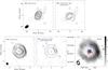 |
Fig. 1 Continuum emission maps at 1.3 mm of the AB Aur region. Top panels:
larger scale image obtained from the SMA data (left panel) and the
residual image after removing the emission detected by the PdBI (right
panel). Contour levels are −2, 2, 4, 6, 8, 10 to 80 by 10 × 1 mJy per
7 |
3.1. Continuum observations
Figure 1 is a montage of our 1.3 mm continuum maps obtained from the SMA and PdBI data.
3.1.1. Large-scale continuum
For the SMA data (upper-left panel in Fig. 1), the total flux is about 110 mJy and the rms noise 1 mJy beam-1. This value is only marginally lower than the single-dish measurement of 130 mJy, made at slightly higher frequency (Henning et al. 1998). Although the emission appears localized toward AB Aur, it does not only originate in the circumstellar disk of AB Aur. The PdBI data only recovers about 80 mJy of the total flux (see below). After removing the ring emission recovered by the PdBI from the SMA data, there is residual emission toward the south of the disk (upper-right panel of Fig. 1).
The excess emission peaks about 14 southeast of AB Aur, and half of the
missing flux is within one SMA beam. There is no significant structure on scales smaller
than about 3′′. Such structures would have been recovered by the PdBI, because it
provides sufficient uv coverage and sensitivity to 2−3′′ scales. This
excess emission is thus smooth on a scale of 3′′ or more. It presumably traces the
remnant envelope of AB Aur.
With a dust absorption coefficient, κ = 0.02 cm2 g-1 (gas+dust) at 230 GHz, which is characteristic of disks (Beckwith et al. 1990), and a dust temperature of 30 K, the total gas mass obtained with the SMA would be 10-2 M⊙. For more pristine, ISM-like dust, the mass would be about four times higher. For the residual emission, the mean NH is 1.3 × 10²³ (cm-2). Assuming the residual emission is spherically symmetric, the mean number volume density nH is 5 × 10⁶ (cm-3).
3.1.2. High angular resolution data
At high angular resolution, the 1.3 mm continuum emission is resolved into three structures (bottom panels in Fig. 1):
-
a continuum peak at the central stellar position;
-
a continuum gap between the central peak and a dust ring;
-
a dust ring/ellipse.
The continuum peak near the center is detected at the level of
5.7σI with a total flux of 1.3 mJy. It is not resolved
within the 037 (50 AU) interferometric beam. This mm
continuum peak also coincides (within the astrometric accuracy of our measurements,
about 005) with the stellar position and the
3.6 cm emission peak (Fig. 1, lower-right panel).
The flux density of the 3.6 cm emission is 0.2 mJy (Rodríguez et al. 2007). With a spectral index of 0.6, characteristic of
optically thick emission in an expanding ionized jet or wind (Panagia & Felli 1975), this would yield 1.5 mJy at 1.3 mm, so
that the 1.3 mm signal from the star position could be purely due to an ionized jet. On
the other hand, optically thin free-free emission would have an essentially flat
spectrum, so the remaining ≈ 1.1 mJy flux could come from dust emission from an inner
disk. A very small (2−3 AU), optically thick, and dust disk would provide enough flux. A
(gas+dust) mass of 4 × 10⁻⁵M⊙ is required for
such inner disk, assuming the temperature of 80 K and
κ = 0.02 cm2 g-1. This mass is likely a
lower limit since the dust emission should be partially optically thick.
The continuum gap (cavity) between this central peak and the dust ring has a width of
~06, corresponding to about 90 AU. It
appears more pronounced in the east and southeast, but this is not statistically
significant.
The dust ring/ellipse confirms the structure found by Piétu et al. (2005). With higher spatial resolution, we are able to further separate the emission from the central star. For an assumed dust temperature T(r) = 50(r/100 AU)0.4 K (see the following paragraph) and κ = 0.02 cm2 g-1, the ring mass is 5.0 ± 0.5 × 10⁻³ M⊙. With the same assumptions as in Sect. 3.1.1, the peak NH and nH of the dust ring are 7.3 × 1025 (cm-2) and 7.0 × 10¹⁰ (cm-3), respectively. The intensity contrast on the dust ring is ≤ 3.
The continuum emission is further fitted using DiskFit with an inclined, sharp-edged
ring, as done for GG Tau (Guilloteau et al.
1999). We fitted two different functionals: a truncated power law given by
 (1)and an exponentially tapered distribution
given by
(1)and an exponentially tapered distribution
given by  (2)The best-fit of the dust ring parameters
are listed in Table 2. Both functionals give
similar results, in particular for the inner radius. The derived surface density
profiles are given in Fig. 2. The tapered edge
solution deserves specific comment. With the large inner radius also found in our
best-fit solution, the high negative value found for the exponent is required to fit the
steep decrease in surface brightness in the outer part. A solution in which both the
inner and outer parts are fit by a profile with no sharp inner radius is possible, but
would imply even more negative exponent values, below −4.5, a situation very similar to
that found by Isella et al. (2010) for MWC 758.
Besides being somewhat better than this solution, our fit demonstrates that the outer
edge is rather sharp and that the dust emission does not extend beyond about 250 AU.
(2)The best-fit of the dust ring parameters
are listed in Table 2. Both functionals give
similar results, in particular for the inner radius. The derived surface density
profiles are given in Fig. 2. The tapered edge
solution deserves specific comment. With the large inner radius also found in our
best-fit solution, the high negative value found for the exponent is required to fit the
steep decrease in surface brightness in the outer part. A solution in which both the
inner and outer parts are fit by a profile with no sharp inner radius is possible, but
would imply even more negative exponent values, below −4.5, a situation very similar to
that found by Isella et al. (2010) for MWC 758.
Besides being somewhat better than this solution, our fit demonstrates that the outer
edge is rather sharp and that the dust emission does not extend beyond about 250 AU.
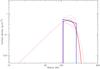 |
Fig. 2 Best-fit surface density distributions for the power-law (blue) and tapered-edge (red) models. Dotted curves represent the ± 1σ of the best-fit value. Without an inner edge, the tapered edge solution would provide too much flux from the inner 100 AU, as shown by the dashed line. |
In addition to these three structures, there is a northeast continuum peak
22 away from the stellar position,
corresponding to the ET peak identified by Lin et al.
(2006) in their 0.88 mm continuum image. It is in between CO S1 and S2 arms
(see Sect. 3.3). The intensity of this northeast
peak is 0.76 mJy beam-1 (3.3σI). Because it is
statistically not significant, we do not discuss this component further.
The center of the dust ring is at
(α,δ)J2000 =
(4h55m45.85s,
30°33′432), consistent with the stellar
location. The position angle (PA) of the rotation axis with respect to north of the
best-fit ring is ~–30°. The inclination angle, i, is ~23°
based on the ratio of minor axis to major axis assuming the ellipse is thin. After
subtracting the ring, the residual image given in Fig. 1 (bottom-middle panel) shows a strong northsouth residual on the western side
and a strong negative residual on the eastern side, suggesting that the emission on the
dust ring is not azimuthally symmetric.
Fitting parameters of dust ring.
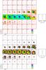 |
Fig. 3 Top panel: 12CO J = 2 → 1 channel
maps from the 30-m observations at 11 |
3.2. CO gas
The channel maps and the spectrum obtained with the IRAM 30-m toward AB Aur are shown in
the top panel in Fig. 3. The angular resolution of
the IRAM 30-m is 112. The emission is extended and dominated
by the envelope near the systemic velocity. There is a velocity gradient in the
southeast-northwest direction. The combined image of the 30-m + SMA CO data with the
smoothed resolution of 74 is presented in the lower panel in
Fig. 3. The peak flux density is 84 Jy
beam-1, which corresponds to 40 K. At this resolution, the emission toward
the south is clearly seen near the velocity of 6.9 to 7.3 km s-1.
3.2.1. Large-scale map at high angular resolution
We present in Fig. 4 the 12CO J = 2 → 1 mosaic image from PdBI. The full data set was also studied, combining the 30-m data with the SMA field and the PdBI mosaic. A comparison between the 30-m+SMA+PdB recombined image and the PdB-only mosaic reveals that all the interesting detected structures are actually confined to within the central beam of the PdBI mosaic, with few significant structures (at high resolution) beyond about 12′′ from AB Aur. Moreover, the extended emission recovered in the 30-m + SMA + PdB image makes the structures less obvious. The PdB-only mosaic channel maps presented in Fig. 4 are more suitable to pinpointing the contrasts between different structures. Since these images do not include the extended flux, the apparent brightness temperatures are lower limits, and correction for the missing flux must, however, be included to derive physical parameters, such as temperature.
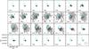 |
Fig. 4 Channel maps of the 12CO J = 2 → 1 line from the PdBI
mosaic. The contours are 1 to 9 by 1 × 0.1 Jy per
0 |
3.2.2. Inner gas
The 12CO J = 2 → 1 emission is detected from the velocity
of 1.6 km s-1 to 9.5 km s-1 (Figs. 4 and 5). The emission peaks in the
high-velocity ends (Fig. 5) are near the 1.3 mm
continuum central peak. The mean position of the highest velocity CO peak is off by
~0 to the 1.3 mm stellar peak. Relative
positions are controlled by the bandpass calibration accuracy, which would yield
relative positions valid to about 1/100th of the beamsize, and by the signal-to-noise.
The difference is at 2 to 3σ level and is only marginally significant.
to the 1.3 mm stellar peak. Relative
positions are controlled by the bandpass calibration accuracy, which would yield
relative positions valid to about 1/100th of the beamsize, and by the signal-to-noise.
The difference is at 2 to 3σ level and is only marginally significant.
High-velocity CO gas (Fig. 5) is detected well within the dust ring, at least as close as 20 AU from the star. This high-velocity emission is consistent with a rotating disk with the rotation axis of PA = −38° ± 1°. However, because of the restricted velocity range (more than 2.4 km s-1 away from the systemic velocity) and limited spatial extent, the inclination angle is poorly constrained.
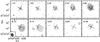 |
Fig. 5 The same as Fig. 3 but toward high-velocity channels. The gray cross marks the
size of the disk (145 AU) with a positional angle of 150°. The contours are
multiples of 44 mJy per 0 |
Best-fit parameters of high velocity CO emission.
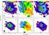 |
Fig. 6 Maps of moments 0, 1, and 2 from left to right panel for 12CO J = 2 → 1 (upper row; this work) and 13CO J = 2 → 1 (lower row; Piétu et al. 2005). The white ellipse and arcs trace the best-fit dust ring and the identified CO spiral arms, respectively. Left panels: The contours start from and step in 0.12 Jy beam-1 km s-1. Middle panels: contours steps are 0.4 km s-1. Right panels: contours steps are 0.1, 0.2, 0.3, 0.4, 0.6, 0.8, 1.0, ... km s-1. The unit of the wedge is Jy beam-1 km s-1 for moment 0 maps and is km s-1 for moment 1 and moment 2 maps. |
Physical quantities based on two inclination angles are further derived and presented in Table 3. We used a simple disk model and the DiskFit code (Piétu et al. 2007) to derive them: the temperature, T, and velocity, V, are assumed to follow a power-law dependence on the radius, r: T = T0(r/r0)−q and V = V0(r/r0)−v. On one hand, if the inclination angle is fixed to 23°, corresponding to the best fit of the continuum ring, the best-fit velocity law will be compatible with Keplerian rotation. The stellar mass (M∗) will be 3.5 ± 0.2 M⊙, which is higher than the mass of 2.4 M⊙ expected from the AB Aur spectral type. On the other hand, if the stellar mass is fixed to be 2.4 M⊙ and the disk is assumed to be in Keplerian rotation, the best-fit inclination angle will be 29°, which deviates from the best-fit value for the dust ring of 23°. Finally, if the inclination angle is fixed to be 29°, the best-fit velocity power-law index becomes v = 0.72 ± 0.03, i.e., the Keplerian rotation assumption is rejected at the 7σ level. We do not find a common model that can fit both the dust ring and high-velocity CO emission.
In comparison, on a larger scale, the rotation axis as derived from 13CO by Piétu et al. (2005) has the PA = −30° ± 1°, which is consistent with the best-fit value of the dust ring. The inclination angle is in between 36° and 42°, which is significantly larger than the values derived from our new high angular resolution data. We note that the velocity field on a large scale is sub-Keplerian. Another puzzling issue is the derived systemic velocity, Vsys. It is 5.73 ± 0.02 km s-1 as derived from the high-velocity parts only and is 5.85 ± 0.02 km s-1 for the outer disk. This difference is marginally significant at the level of 4σ. Such a deviation in Vsys may be due to an asymmetry in brightness between the blue- and red-shifted wings, reflecting that the distribution of the gas is inhomogeneous.
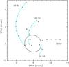 |
Fig. 7 Locations on the spirals where the spectra in Fig. 8 are taken. The 1.3 mm dust ring is marked as a black ellipse. |
3.2.3. The disk
The integrated intensity (moment 0), the intensity weighted velocity (moment 1), and the intensity weighted linewidth (moment 2) maps of 12CO J = 2 → 1 from this work and of 13CO J = 2 → 1 by Piétu et al. (2005) are shown in Fig. 6. As a reference, a white solid ellipse that marks the 1.3 mm dust ring is also indicated. Figure 6 shows that 12CO emission is much more extended (7′′ or 1000 AU) than 13CO, which is strongly dominated by the rotating disk, and extends out to 4′′ (560 AU). The outer radius in continuum is even smaller, at most 280 AU (see Fig. 2). While opacity differences naturally produce this ordering (R(dust) < R(13CO) < R(12CO)), the sharpness of the dust profile would lead to only marginally larger radii for 13CO and 12CO if opacities only were to explain this result. Our result thus confirms and reinforces the proposition made by Piétu et al. (2005) of a change in dust properties (emissivity or gas-to-dust ratio) at a radius around 280 AU. Our more precise determination is now in excellent agreement with the feature detected at 20 μm by Pantin et al. (2005). This suggests that a change in dust properties is more likely than a drop in gas-to-dust ratio beyond 280 AU.
3.3. Spiral structure
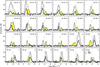 |
Fig. 8 Spectra of 12CO 2−1 (thin line) and 13CO 2−1 (thick line) on
the locations of CO spirals. The alphabet order labels the distance to the stellar
location: A is the closest, while J is the most distant one. The
separations between the spectra is 0 |
3.3.1. Identification of the spiral arms
The 12CO moment maps exhibit very different morphology from those of 13CO (from Piétu et al. 2005). While 13CO traces the rotating disk, there are spiral-like patches with broader velocity dispersion and excess integrated intensity compared to the Keplerian patterns in the 12CO line.
The 12CO moment 0 and moment 2 maps from Fig. 6 allow us to identify four “spiral” patterns, CO S1 to CO S4. From the moment
2 image, there are three patches where the linewidths are broader. We marked them as CO
S1 to CO S3. Part of these arms can also be seen in the moment 0 map. Although the
linewidth of CO S4 is not as broad as CO S1 to CO S3, there is excess emission at S4 in
the moment 0 map. Besides the 05 maps, we also checked the
12CO J = 2 → 1 maps with different tapering. The excess
emission near the spirals can still be seen but is not as obvious as in the
05 maps. On larger scales, the
12CO line might be too contaminated by the emission from the envelope in
the combined maps. Another reason might be that the excess emission comes from
structures that are actually very compact and not as bright as the Keplerian disk
emission. We note that the labeled spirals are traced by first marking the locations
where the moment 0 and moment 2 maps clearly show excess emission “by eye”. Then, we fit
four parabolic arcs to the marked locations.
We further checked the spiral emissions in the channel maps (Fig. 4). The S1 and S2 arms are on the blue-shifted part of the disk. In S1, the spiral emission can be seen at 3.9 to 6.7 km s-1. The S2 arm is the most extended spiral among these four arms: it appears from 4.7 to 7.3 km s-1 and connects to the SE part of the disk. The S3 and S4 arms are on the red-shifted part and at the near side of the disk. The S3 arm has the broadest linewidth and it shows up from 4.3 to 7.3 km s-1. The S4 arm appears from 5.7 to 7.7 km s-1. The bases of the four spiral arms are different. The S1 arm seems to trace back to the 1.3 mm gap (cavity; see the channels 3.9 to 5.5 km s-1 in Fig. 4 and moment 2 in Fig. 6). The S3 arm can be traced back to the ring inner edge (see channels 4.3 to 4.9 km s-1 in Fig. 4). S2 and S4 arms originated somewhere near the dust ring. The connection of these CO spirals with the dust ring and the NIR spirals and the comparison with the spirals detected in CO 3−2 will be discussed in Sect. 4.3.1.
Spectra of 12CO J = 2 → 1 and
13CO J = 2 → 1 line along the spirals at locations spaced
every 056 (see Fig. 7 for point labeling) are given in Fig. 8. While the 13CO J = 2 → 1 line shows only the
emission from the (nearly) Keplerian disk, the
12CO J = 2 → 1 spectra clearly exhibit a new kinematic
component. The 12CO J = 2 → 1 spectra can be decomposed into
two Gaussians, one of which traces the rotating disk (at almost the same velocity as the
13CO J = 2 → 1 line) and the other traces an excess
emission on the spiral. They are named 12COdisk and
12COspiral, respectively. Results of the Gaussian best-fit are
listed in Table 4, and the kinematics are
discussed in Sect. 4.2.3. The velocity offsets of the two Gaussians are typically 1 to
2 km s-1. This provides a natural explanation of the apparent broad
linewidths in the spiral locations: there is a bulk of gas moving at different
velocities from the rotating disk but not because of turbulent motions on the spirals.
We note that although the spirals (arcs) are labeled by eye and not based on
quantitative criteria, the parameters derived in this way are expected to reflect the
bulk properties of these non-Keplerian component.
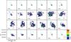 |
Fig. 9 The line ratio of 13CO J = 2 → 1 to 12CO J = 2 → 1 as a function of position in different velocities. There is some self-absorption (red color) in the southern parts. The 13CO emission otherwise has < 1 optical depth. |
3.3.2. Temperature and opacity
The peak temperature in the CO maps, around 80 K, and the average brightness temperature in the inner 11″, 40 K, indicate temperatures ranging from 30 K outside to 100 K in the inner regions of the disk, confirmed by the more sophisticated disk analysis presented in Table 3.
The CO line opacity can be estimated from the 13CO/12CO ratio map (Fig. 9). On large scales, in the velocity channels 5.22 to 6.72 km s-1 in the southern part, and 4.97 to 5.47 km s-1 in the northeast of the disk, the ratio 13CO/12CO is over 1 (Fig. 9). This must be due to self-absorption in 12CO, implying optically thick in 13CO with a temperature decreasing as a function of distance from AB Aur.
On the identified CO spirals, the 13CO/12CO ratio is low (in fact there is no robust 13CO detection), so the 12CO opacity cannot be very high. A better constraint comes from the apparent brightness temperature of the emission, which ranges from 10 K to 30 K. Assuming the kinetic temperature in the spiral is comparable to the one in the disk, this moderate brightness indicates opacities of 0.3 to 1, since the spirals are resolved. Higher temperatures (hence lower opacities) cannot be excluded, but this would require a multiline study.
3.3.3. Gas mass and energetics inside the spirals
Under LTE conditions, the column density of the CO spirals can be estimated using the
standard equation 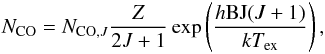 (3)where
NCO,J is the column density of the CO
molecule in the quantum state J
(J + 1 → J). Here,
NCO,J is given by
(3)where
NCO,J is the column density of the CO
molecule in the quantum state J
(J + 1 → J). Here,
NCO,J is given by
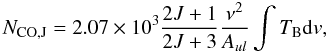 (4)where B,
ν, Aul, and
TB dv are the rotational constant, the
frequency in GHz, the spontaneous transition rate, and the brightness temperature
TB in K integrated over the linewidth dv
in km s-1, respectively. Here, Z is the partition
function,
(4)where B,
ν, Aul, and
TB dv are the rotational constant, the
frequency in GHz, the spontaneous transition rate, and the brightness temperature
TB in K integrated over the linewidth dv
in km s-1, respectively. Here, Z is the partition
function,  (2J + 1)
exp[− hBJ(J + 1)/kTex],
and Tex is the excitation temperature.
(2J + 1)
exp[− hBJ(J + 1)/kTex],
and Tex is the excitation temperature.
We assume Tex = 50 K as representative of the average
temperature inside the arms. The derived column density of 12CO and
13CO in the spirals are thus given by
N12CO = 8.9 × 10¹³ dv and
N13CO = 6.07 × 10¹³ dv, respectively. With
the integrated line flux calculated using TB and
△ v given in Table 4, the
derived values of
dv and
N13CO = 6.07 × 10¹³ dv, respectively. With
the integrated line flux calculated using TB and
△ v given in Table 4, the
derived values of  range from 1.5 × 10¹⁴ to
1.5 × 1015 cm-2. Using a CO/H2 ratio of
10-4, the total gas mass in these four spirals is only
2.5 × 10⁻⁷ M⊙. Opacity effects could increase
these values.
range from 1.5 × 10¹⁴ to
1.5 × 1015 cm-2. Using a CO/H2 ratio of
10-4, the total gas mass in these four spirals is only
2.5 × 10⁻⁷ M⊙. Opacity effects could increase
these values.
An upper limit of the total mass of the spirals can be estimated from the
13CO J = 2 → 1 line, which is not detected in the spirals.
With the 3σ noise level of 3 K per channel (0.25 km s-1),
 is less than 1014
cm-2, assuming the same linewidth as
12CO J = 2 → 1. Assuming the 12C/13C
ratio 77 in the local ISM (Wilson 1994), the
upper limit of
is less than 1014
cm-2, assuming the same linewidth as
12CO J = 2 → 1. Assuming the 12C/13C
ratio 77 in the local ISM (Wilson 1994), the
upper limit of  and the gas mass in the spirals are
~1016 cm-2 and
1.5 × 10⁻⁵ M⊙, respectively. In comparison,
in the disk at 100 AU estimated in Piétu et al. (2006) is
1.4 × 1019 cm-2. In the spirals, the column density is at least
103 times lower than the one in the disk.
and the gas mass in the spirals are
~1016 cm-2 and
1.5 × 10⁻⁵ M⊙, respectively. In comparison,
in the disk at 100 AU estimated in Piétu et al. (2006) is
1.4 × 1019 cm-2. In the spirals, the column density is at least
103 times lower than the one in the disk.
Parameters of the Gaussian best-fit toward 13CO and 12CO.
The kinetic energy contained in the spirals in the rotating disk frame are calculated
using the equation 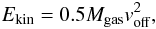 (5)where voff is
the difference between the VLSR of the
12COspiral component and the VLSR of
the 13CO component listed in Table 4.
The resulting Ekin on the spiral is 6 × 1036 erg.
The upper limit of Ekin given from
13CO J = 2 → 1 is 3 × 1038 erg, assuming the
same voff as the 12COspiral component
with the estimated upper limit of the spiral mass.
(5)where voff is
the difference between the VLSR of the
12COspiral component and the VLSR of
the 13CO component listed in Table 4.
The resulting Ekin on the spiral is 6 × 1036 erg.
The upper limit of Ekin given from
13CO J = 2 → 1 is 3 × 1038 erg, assuming the
same voff as the 12COspiral component
with the estimated upper limit of the spiral mass.
If the gas on the spirals mainly moves on the disk plane, the reported energy will be a factor of six higher, assuming that the inclination angle is 23°. In comparison, the binding energy of a companion with a mass of 0.03 M⊙ at 45 AU, is 2.4 × 1043 erg, which is at least four orders of magnitude greater than the kinetic energy contained in the spirals. A small perturbation of the orbit of such a companion is sufficient to release enough energy to sustain such spirals. If emission is at a larger h and is optically thick, the estimated Ekin will be the lower limit. The angular momentum is estimated to be 1047 in cgs following the same method.
4. Discussion
At high angular resolution both in the NIR and the submm domains, the surroundings of AB Aur are complex. Figure 10 is a montage of the 1.3 mm continuum image with CO spirals, the optical image from HST, and the NIR image from HiCIAO of Subaru telescope. Superposed are the spirals as determined from the NIR by Hashimoto et al. (2011) and the CO spirals (this work). The HST image from Grady et al. (1999) on large scales also reveal the spiral arms, which were later reported closer to the central star by Fukagawa et al. (2004) from Subaru deep images.
In dust emission, the large inner cavity and well-defined dust ring appear much like a scaled-down version of the tidal cavity+ring observed in the binary system GG Tau/A (Guilloteau et al. 1999). More recently, several SMA, CARMA, and IRAM PdBI observations have revealed the existence of such large cavities inside disks, such as HD 135344B, MWC 758, LkCa 15, or even HH 30. The material around AB Aur also differs from similar objects in some important aspects:
-
In the large-scale CO emission, four spiral-like arms are detected.Part of these CO spirals are also seen in NIR eventhough the existence of a remaining envelope of dust, whichaffects NIR image mostly, and gas (12CO) partially contaminates anydetailed analysis of the material close to the star.
-
The disk is not in Keplerian rotation, and the dust ring is clearly asymmetric both in continuum and in the 12CO and 13CO lines.
-
The inner cavity is not fully devoid of gas. This gas is likely not uniform within the central hole (see Sect. 3.2.2).
-
Fitting the large-scale disk traced in 13CO and C18O (see Sect. 4.2.1) and the dust ring separately leads to some apparent inconsistencies. In particular the inclination angles differ from 42° to 23° (while the typical errors are 1° to 3°).
In this section, we discuss these points and see how they can be interpreted and possibly reconciled in a single picture. We focus first on a comparison of the mm/submm data with other similarly resolved observations and on the ring properties. We then discuss an overall scheme for the spiral features and present the dynamics of the AB Aur system.
4.1. Properties of the ring and inner material
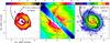 |
Fig. 10 Left panel: dust continuum at 1.3 mm (color scale) and CO spirals
(black arcs). Middle panel: HST image (color scale) and CO spirals.
The 1.3 mm dust ring is marked as a white ellipse. Right panel:
comparison of 1.3 mm continuum (contours) and the HiCIAO polarization intensity (PI)
image (color scale) at NIR. The black and red arcs mark the CO spirals identified in
Fig. 6 and the HiCIAO arm (Hashimoto et al. 2011), respectively. The S1 arm
is marked as a solid arc, because it is the one with apparent corresponding
CO spirals. The coronagraphic occulting mask of
0 |
4.1.1. Dust gap and inner material
The 1.3 mm continuum peak at the stellar location might suggest the existence of, at least, one inner disk. The lower limit of the total gas+dust mass at the stellar location is estimated to be 4 × 10⁻⁵ M⊙ (Sect. 3.1.2). Although we cannot rule out the possibility that the 1.3 mm stellar peak comes from the optically thick free-free emission, an inner disk has been detected and resolved in the near infrared (NIR) and mid-infrared (MID-IR) interferometric observations by Eisner et al. (2004) and di Folco et al. (2009). The inner disk is also required to explain the observed accretion rate of 10-9 to 3 × 10⁻⁷ M⊙ yr-1 (Brittain et al. 2007; Telleschi et al. 2007; Donehew & Brittain 2011).
Besides the continuum emission at the stellar location, the detection of “high” velocity 12CO J = 2 → 1 emission inside the dust cavity also indicates that this area is not devoid of gas. The gas mass estimated from the CO 2−1 line with velocity more than 2.5 km s-1 away from Vsys is ~10-5M⊙. These gases are 50 AU away from the stellar location with an orbital period of 200 yr. From the orbital timescale argument, which the mass accretion rate toward the center cannot exceed the orbiting mass divided by the orbiting period, the upper limit of the accretion rate is in the order of 10-7M⊙ yr-1, consistent with the values reported in previous paragraph.
4.1.2. Ring properties
Comparing the 1.3 mm continuum with NIR emission is not straightforward, because the dust disk has very high optical depth at NIR. The dust emission at these two wavelengths originates in different dust layers. The NIR emission traces the scattered-stellar light by dust grains in the upper layers of the flared disk, while the 1.3 mm thermal emission, which is essentially optically thin, characterizes the bulk of the disk mass. Although the very inner parts of the NIR maps are occulted (e.g. HiCIAO data: the area of the mask is seen in white in Fig. 10), the superposition of the mm and infrared images reveals coherent behavior (Fig. 10). We find that the NIR emission peaks before the mm ring at radius around 70 AU, then the mm emission peaks at radius 150 AU followed by a decrease in the NIR brightness, indicating that there are fewer stellar photons impinging on the disk behind the bulk of the dust emission. This behavior is fully consistent with predictions from stellar irradiated-dust disk models (see for example, Dullemond et al. 2007).
The AB Aur disk is not azimuthally homogeneous. The best-fit models derived from the 1.3 mm and the 12CO data in Tables 2 and 3 assume uniform density distribution with azimuth. The residual image of the 1.3 mm continuum (i.e. after subtracting the best-fit ring; lower middle panel of Fig. 1) clearly shows the inhomogeneity in both radius and azimuth. The azimuthal asymmetry can be quantified by Fig. 11 where we trace the dust intensity at 1.3 mm versus the position angle with respect to the major axis of the disk, θPA (measured in the disk plane, by assuming an inclination of 23 °), inside the ring (peak location, Fig. 1). The major axis of the disk is assumed to be −121.3° from north, since the disk rotation axis is at −31.3° from the best fit of 13CO in Piétu et al. (2005). There are two dips in the ring, one at θPA of 130° and the other at −150° (Fig. 11). The emission peak is at θPA of about 30°. The maximum intensity contrast on the ring is about 3.
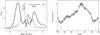 |
Fig. 11 Left panel: plot of the normalized intensity of 1.3 mm continuum
and HiCIAO PI image at NIR along the major axis of the disk’s major axis. The
central 0 |
4.2. CO disk
4.2.1. Inclination angle
The determined inclination angle i of AB Aur disk varies with scale. For the inner disk (radius ≥ 20 AU), i is 23° to 29° based on the high velocity 12CO J = 2 → 1 line (Sect. 3.2.2; Table 2). With the best-fit dust ring at 1.3 mm (radius of 145 AU), i is 22° to 24° (Sect. 3.1.2; Table 1), consistent with the inclination derived from the high-velocity 12CO line. We note that the derived inclination angle from the 12CO J = 2 → 1 data is based on the high-velocity components (2.4 km s-1 offset from the Vsys), which are less likely to be contaminated by the envelope. On a larger scale (radius 70 AU to 600 AU), Piétu et al. (2005) reports i to be 36° based on the C18O J = 1 → 0 line. Because the C18O J = 1 → 0 line is optically thin and also less likely to be contaminated by the large-scale envelope, the discrepancy between the values derived from 12CO and C18O suggests a physical warp. We note that the low i toward a smaller scale has already been reported. Based on the NIR interferometric data, Eisner et al. (2004) find that i is ≤ 20° for an inner disk with a radius less than 1 AU. The i inferred from our new 1.3 mm continuum and CO data is more consistent with the value derived from the NIR.
Warped disks have been reported in the literature, e.g., Beta Pictoris (Golimowski et al. 2006, and references therein). The AB Aur system is somewhat similar to the GG Tau A system. Guilloteau & Dutrey (2001) show the high angular resolution 12CO J = 2 → 1 observations of CO gas inside the cavity with slightly different inclination angle from the one derived from the dust ring.
4.2.2. Rotation
The rotation velocity also varies with scale. In Piétu et al. (2005) and Lin et al. (2006), the CO emission was found to be in non-Keplerian rotation. This is partly due to the confusion with the remaining envelope since the 12CO J = 2 → 1line and especially the 12CO J = 3 → 2 line are mostly optically thick, tracing both the envelope and the disk. However, observed with 13CO and C18O, where confusion is negligible, Piétu et al. (2005) measured the velocity power-law exponents v of 0.42, 0.37, 0.47, and 0.82 for 13CO J = 2 → 1, 13CO J = 1 → 0, C18O J = 2 → 1, and 12CO J = 2 → 1, respectively. These exponents were fitted with all the detected emission in Piétu et al. (2005), which is probably dominated by the larger scale disk. The new 12CO J = 2 → 1 data at higher angular resolution add an additional puzzle, since the velocities within 100 AU appear to exceed the orbital velocity around a ~2.4 M⊙ mass star. One might explain such high velocities with an increasing inclination angle at smaller radius, but the implied disk warp is opposite to the one discussed in Sect. 4.2.1 above. Given the possible brightness asymmetry (see Sect. 3.2.2), a better explanation is perhaps that the interpretation in terms of Keplerian disk is totally inappropriate. Instead, this gas may be tracing streamers of gas infalling (and rotating) from the ring onto the central object.
4.3. CO spirals
Our observations show that the disk structure in AB Aur is highly asymmetric. Although sensitive CO 3−2 and CO isotopes are still needed to better constrain the temperature and density on the spirals, our data provide the dynamics of this morphological component for the first time.
4.3.1. Geometry
Spiral-like structures have been detected both in the CO gas and the dust emission/scattering light at various wavelengths, although they do not come from exactly the same locations. In the IR, Fukagawa et al. (2004) report four spirals (one inner arm, two outer arms with a branch on one of the outer arms). More recently, Hashimoto et al. (2011) identified eight spirals, namely S1, S2, ..., S8, based on the infrared polarization-intensity image. In comparison, the CO S2 shares part of the base with the infrared S1 (inner arm in Fukagawa’s spiral) and S2 arms, which are in the southern part of the 1.3 mm dust ring (Fig. 10). The CO S3 arm seems to trace the inner part of infrared S3 sprial (Fukagawa’s outer arm). We note that the spiral detected at 5.68 km s-1 in CO 3−2 by Lin et al. (2006) appears in between CO S1 and CO S2 and traces the NIR S1 spiral more, suggesting that it is at a more upper layer than the CO 2−1 spirals.
In NIR, the spirals located in the southern region appear shorter, suggesting an inclination effect on a geometrically flaring structure. The spirals closer to us are compressed compared to those located on the other side. This is also consistent with the NIR data, which reveal that the southern part is brighter and thus closer (forward scattering). To constrain the physical conditions of the spirals, high angular-resolution and high-sensitivity observations of 12CO and 13CO at multiple J states are needed.
4.3.2. Gas kinematics
So far, we only have the velocity information along the line of sight. Assumptions
about the 3D geometry are required to recover further information. Starting from the
disk geometry, the observed velocity of gas motions with respect to the local standard
of rest (LSR), VLSR, can be decomposed in cylinder
coordinate (r, θPA,z):
![Mathematical equation: \begin{eqnarray} \label{eq:vlsr} V_{\rm LSR} & = & V_{\rm sys} + [V_{\rm rot}(r){\rm cos}(\theta_{\rm PA}) + V_{\rm rad}(r){\rm sin}(\theta_{\rm PA})]{\rm sin}(i) \nonumber \\ &&+ V_{\rm z}(r) {\rm cos}(i), \end{eqnarray}](/articles/aa/full_html/2012/11/aa19414-12/aa19414-12-eq180.png) (6)where Vsys is
the systemic velocity with respect to LSR. We chose 5.85 km s-1 for AB Aur in
this calculation, because the spiral-like structures are extended. Here,
Vrot is the rotation velocity (positive in
counter-clockwise), while Vrad (positive for outward
motions) is the radial velocity in the disk plane, and
Vz is the component perpendicular to
the disk plane. The symbol θPA is the position angle of each
location with respect to the major axis of the disk (− 121.3° from the north),
and i is the inclination angle of the disk axis with respect to the
line of sight. When calculating θPA in each location of
spirals, we assume i = 23°, because this best-fit model gives a
Keplerian disk (see Table 3).
(6)where Vsys is
the systemic velocity with respect to LSR. We chose 5.85 km s-1 for AB Aur in
this calculation, because the spiral-like structures are extended. Here,
Vrot is the rotation velocity (positive in
counter-clockwise), while Vrad (positive for outward
motions) is the radial velocity in the disk plane, and
Vz is the component perpendicular to
the disk plane. The symbol θPA is the position angle of each
location with respect to the major axis of the disk (− 121.3° from the north),
and i is the inclination angle of the disk axis with respect to the
line of sight. When calculating θPA in each location of
spirals, we assume i = 23°, because this best-fit model gives a
Keplerian disk (see Table 3).
 |
Fig. 12 Plot of θPA versus ykep (θPA) as defined in Eq. (7) of 13CO,12COdisk, 12COspiral and a purely Keplerian rotation in corresponding colors. The best-fit of each component is shown as a curve. |
In this decomposition, motions perpendicular to the disk plane would not depend on θPA. The symmetric motions perpendicular to the disk midplane cannot be seen: these would only add up velocity dispersion after considering the limited angular resolution, but not change the projected mean velocity.
For pure Keplerian rotation, Vrot equals
 , where M is the
enclosed mass within a radius r, and Vrad
and Vz are 0. Equation (6) can be rearranged as
, where M is the
enclosed mass within a radius r, and Vrad
and Vz are 0. Equation (6) can be rearranged as  (7)where
ykep(θPA) now only depends on
cos(θPA).
(7)where
ykep(θPA) now only depends on
cos(θPA).
Similarly, if we can correct for radial dependencies, pure radial motions would vary as
sin(θPA). For example, for free-fall accretion in the disk
plane, Vrad equals  , Vrot and
Vz are 0. Equation (6) can be rearranged as
, Vrot and
Vz are 0. Equation (6) can be rearranged as  (8)Thus, a display of
![Mathematical equation: \hbox{$y = [V_{\rm LSR}-V_{\rm sys}] \sqrt{r}$}](/articles/aa/full_html/2012/11/aa19414-12/aa19414-12-eq192.png) as a function of
θPA can reveal the relative contributions of (Keplerian)
rotation and other motions. We fitted 1) a pure rotation
y = a1cos(θPA − a2);
and 2) a combination of rotation and radial motions
y = a3cos(θPA) + a4sin(θPA)
to the observed velocities in the spirals. We excluded Location 1E from the fit, because
the two velocity components are not separated well here. We also exclude CO S4 in the
fitting, because there is less excess emission on the spirals. The fitting results of a
pure rotation are shown in Fig. 12 and in Table
5. For illustration, a pure Keplerian rotation
with M = 2.4 M⊙ (based on the spectral
type of AB Aur) and i = 23° (based on the axis ratio of the dust ring)
is also shown. We note that this choice of a representable Keplerian rotation in AB Aur
is not trivial, because we do not find a consistent model based on our 1.3 mm continuum
map and the high-velocity 12CO J = 2 → 1 line (see
Sects. 3.1.2 and 3.2.2). Nevertheless, the chosen M of
2.4 M⊙ and i of 23° can describe the
general trend of the derived y values of the 12CO disk
component and also the 13CO line. We also plot a Keplerian rotation with
M = 2.4 M⊙ but with
i = −20° in Fig. 12 in order to
demonstrate that the 12CO spiral component can originate in
corotating gas with high inclination angle with respect to the disk plane. See
Sect. 4.4 for more discussion.
as a function of
θPA can reveal the relative contributions of (Keplerian)
rotation and other motions. We fitted 1) a pure rotation
y = a1cos(θPA − a2);
and 2) a combination of rotation and radial motions
y = a3cos(θPA) + a4sin(θPA)
to the observed velocities in the spirals. We excluded Location 1E from the fit, because
the two velocity components are not separated well here. We also exclude CO S4 in the
fitting, because there is less excess emission on the spirals. The fitting results of a
pure rotation are shown in Fig. 12 and in Table
5. For illustration, a pure Keplerian rotation
with M = 2.4 M⊙ (based on the spectral
type of AB Aur) and i = 23° (based on the axis ratio of the dust ring)
is also shown. We note that this choice of a representable Keplerian rotation in AB Aur
is not trivial, because we do not find a consistent model based on our 1.3 mm continuum
map and the high-velocity 12CO J = 2 → 1 line (see
Sects. 3.1.2 and 3.2.2). Nevertheless, the chosen M of
2.4 M⊙ and i of 23° can describe the
general trend of the derived y values of the 12CO disk
component and also the 13CO line. We also plot a Keplerian rotation with
M = 2.4 M⊙ but with
i = −20° in Fig. 12 in order to
demonstrate that the 12CO spiral component can originate in
corotating gas with high inclination angle with respect to the disk plane. See
Sect. 4.4 for more discussion.
Despite the previously noted apparent deviations from Keplerian motions (best-fit
velocity exponent 0.42, Piétu et al. 2005), the
disk component is very close to pure Keplerian rotation, because the best-fit value
a2 of  and
and
 are 3° ± 4° and 2° ± 5°, respectively.
The kinematics of the spiral component shows more deviations from a simple cosine
function. To the first order, it is fitted with a similar
a2 ≃ 0 but with negative velocity. In other words, the
kinematics of the spiral is apparently dominated by rotation in the opposite
direction to the disk spin, with little contribution from radial motions.
This is confirmed by the fit of rotation + radial motions. The best fit gives
a3 of −1.09 ± 0.10, which is
≃ a1, and a4 of 0.41 ± 0.22,
which is only marginally different from 0. That a4 is 2.5
times smaller than a3 suggests that the motions within the
spirals are mainly rotation with slightly radial motions.
are 3° ± 4° and 2° ± 5°, respectively.
The kinematics of the spiral component shows more deviations from a simple cosine
function. To the first order, it is fitted with a similar
a2 ≃ 0 but with negative velocity. In other words, the
kinematics of the spiral is apparently dominated by rotation in the opposite
direction to the disk spin, with little contribution from radial motions.
This is confirmed by the fit of rotation + radial motions. The best fit gives
a3 of −1.09 ± 0.10, which is
≃ a1, and a4 of 0.41 ± 0.22,
which is only marginally different from 0. That a4 is 2.5
times smaller than a3 suggests that the motions within the
spirals are mainly rotation with slightly radial motions.
Best fit of ykep(θPA).
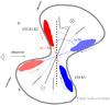 |
Fig. 13 Illustration of the origin of the spiral emissions. The flared disk is plotted in gray segments and arcs. The solid filaments are the detected CO spirals. The hatched filaments with relatively larger inclination angles are not detected. The thick lines mark the large-scale, flattened, and tilted infalling envelope. |
4.4. Overall picture of the AB Aur system
Gas and dust clearly indicate the existence of an inner cavity, of radius ≃ 100 AU. As AB Aur is a strong UV emitter, a possible explanation of such a cavity could be photoevaporation. Following Alexander et al. (2006), a transitional “hole” can appear during the evaporation of the disk. The disk mass in AB Aur is ~0.01 M⊙, which is a factor of ten more massive than in their model. In addition, the inner disk is not completely evaporated since it has been detected at NIR. The high accretion rate of AB Aur (~10-7 M⊙ yr-1) furthermore suggests that the inner disk is still replenished. This inner disk can provide substantial attenuation for ionizing radiation from the central star, and photoevaporation cannot be the dominant process in clearing the disk. Besides, the asymmetry of the dust ring has no simple explanation in this scenario. The AB Aur disk probably cannot be explained by such a model.
An alternative formation mechanism of the gap/cavity is that the disk is in tidal
interaction with an embedded companion or (proto-)planet. Accounting for the inner disk,
the width of the continuum gap is ~90 AU. Resonant motions with a companion in the
gap can produce high-contrast inhomogeneities (e.g. Kuchner & Holman 2003), which would naturally explain the observed azimuthal
brightness variations in the ring. However, the companion mass should be high enough so
that the gap can remain mostly clear of gas or dust, as in the simulation work of Kley et al. (2001). Following Takeuchi et al. (1996), the half-width of a gap, w,
opened by a low-mass companion in the case of a circular orbit can be estimated from:
w = 1.3 r A1/3, where
r is the semi-major axis of the companion orbit and A
the strength ratio of tidal to viscous effects given by
A = (Mp/M∗)2(3α(h/r)2)-1.
With standard values for the ratio of the scale height h to the orbit
radius r, h/r ~ 0.1 and the
viscosity parameter, α, ~0.01 and assuming a stellar mass,
M∗ of 2.4 M⊙, a gap of
half-width w of 45 AU located at r ≃ 45 AU can be opened
by a body of mass Mp ≃ 0.03 M⊙.
However, Hashimoto et al. (2011) rule out
companions more massive than about five Jupiter masses from IR polarization intensity
images. Based on an extreme assumption, 100% of polarized emission for the planet, this
may lead to a low value of the upper limit. Nevertheless, having one or multiple lower
mass bodies in eccentric orbit or a lower viscosity (since the minimum mass scales as
 ) may partially alleviate these
discrepancies.
) may partially alleviate these
discrepancies.
Although the NIR spirals appear more consistent with a simple flared disk model, we cannot explain the CO spirals with such a model. At NIR wavelengths, opacity prevents us from seeing throughout the disk, and we only see the front surface. In the northern part (the farside), the front surface is projected at a lower inclination angle, while in the southern part (the nearside), it is projected at a higher inclination angle. This results in a compression of the NIR spirals toward the south (see Fig. 13 for an illustration). However, the CO opacity at the spiral velocities is moderate, so we could in principle see throughout the disk. An explanation of the CO velocities in terms of different inclinations of the front and back surfaces of a flared disk would only be possible if we saw two anomalous velocity components symmetrically placed around the normal disk velocity. The CO spirals must originate in a structure that is more complex than a flared disk.
Are the CO spirals body-driven? It has been shown numerically that a companion in a disk is expected to drive a single-armed spiral wake (e.g. Ogilvie & Lubow 2002). The multiple arcs/spiral arms observed in the NIR and mm appear difficult to reconcile with a single companion. Multiple bodies spread between distances ranging from 30 to 70 AU would offer a better alternative. However, the pitch angle of such spirals is typically very small. The biggest difficulty with the body-driven spiral pattern is the apparent retrograde motion of the gas. This cannot be obtained with purely in-plane motions. The easiest explanation for the change of the sign in velocity is an inclination angle difference. This could relate to the indications of disk warp. In the multiple-body hypothesis, resonant interaction between these bodies may pump up orbital inclination (and eccentricity) changes, and perhaps more naturally lead to highly (>35°) inclined spiral patterns. However, simulations of multiplanet + disk systems have shown that inclination and eccentricity are in general damped quite efficiently in such cases (see review by Kley & Nelson 2012, and references therein). Finally, we note that density contrast in companion-driven density waves is generally significant (10% to 30 % or so), while the features we have detected here in CO are much fainter.
Counter-rotating gas and spiral pattern may also trace a recent fly-by. Such an event would naturally induce a significant warp in the disk (Nixon & Pringle 2010). Traces of the event are, however, expected to decay on a timescale tdamp ≃ Pout(2/π/α) (Lubow et al. 2002), where Pout is the orbital period at the edge of the outer disk. The tdamp is on the order 106 yr for α = 10-4. Piétu et al. (2005) suggest that two young stars might have had an encounter with AB Aur on such a timescale, JH433 (Jones & Herbig 1979) at any time older than 35 000 years ago, and RW Aur some 500 000 years ago. In this respect, it is interesting to note that RW Aur is a very peculiar T Tauri star binary (1.5 M⊙ for the primary, 0.8 M⊙ for the secondary, Woitas et al. 2001), with a high accretion rate, which exhibits clear evidence of tidal interactions between the two stars, suggesting an eccentric orbit (Cabrit et al. 2006). However, the proper motion measurement accuracy of the suggested fly-by stars precludes accurate conclusions.
An additional important piece of information of the kinematics provided by our observations is the mis-alignment between the “large-scale” (>2000 AU) velocity gradient in the cloud and the AB Aur disk axis. If interpreted by rotation, it indicates that the specific angular momentum of the surrounding envelope projects nearly perpendicular to the AB Aur disk axis. Material from this envelope should thus accrete with very different kinematics from that of the disk, perhaps explaining the apparent counter-rotating spirals.
The large-scale velocity gradient might also be interpreted by infall
motions. From the scattered light images, the southern part is closest to us, and
from Fig. 3, this gas is indeed red-shifted as
expected for infall. The CO spirals could be traces of enhanced accretion along filaments.
In the simplest model, which assumes infall from an envelope with rigid-body rotation,
accreting material is expected to follow quasi-parabolic, nonintersecting orbits (Cassen & Moosman 1981). In this case, our “spirals”
may just trace some parts of such parabolic orbits, and their apparent geometry remains
consistent with such an interpretation. In the orbit plane, the pitch angle of the
“spirals” is given by the ratio of radial to rotational velocity
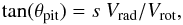 (9)where s is a sign that
depends on conventions for velocities. This intrinsic pitch angle can be recovered from
the “spiral” geometry by assuming some inclination angle i for the orbit
plane. For |i| < 30°, the correction for inclination will remain
small. The shape of our “spirals” is consistent with apparent counter-clockwise rotation
(i.e. direct rotation in the left-handed RA, Dec system) and inward motions. For
i ≃ −20°, i.e. an orbit plane inclined by about 45° compared to the
main quasi-Keplerian disk of AB Aur at i = + 23°, this direction of
rotation is consistent with the overall rotation of the system. The infall motions then
contribute to red-shifted gas along the line of sight in the northern regions (CO Spiral
S1 and S2) and blue-shifted gas in the southern part (CO S3). For S4, which lies close to
the disk’s major axis, the projection of the infall motions would essentially be zero.
This behavior is entirely consistent with the observed velocity shifts in Fig. 8. In addition, the ykep
values of the 12CO spiral component follow the trend of a pure
Keplerian rotation with M of 2.4 M⊙ and
i of −20° (Fig. 12), suggesting
that the spiral gas develops from a higher inclination with respect to the disk plane. The
analysis combining both rotation and radial motion suggests that the gas motion within the
spirals are mainly rotation with slightly radial motion. A schematic is given in
Fig. 13.
(9)where s is a sign that
depends on conventions for velocities. This intrinsic pitch angle can be recovered from
the “spiral” geometry by assuming some inclination angle i for the orbit
plane. For |i| < 30°, the correction for inclination will remain
small. The shape of our “spirals” is consistent with apparent counter-clockwise rotation
(i.e. direct rotation in the left-handed RA, Dec system) and inward motions. For
i ≃ −20°, i.e. an orbit plane inclined by about 45° compared to the
main quasi-Keplerian disk of AB Aur at i = + 23°, this direction of
rotation is consistent with the overall rotation of the system. The infall motions then
contribute to red-shifted gas along the line of sight in the northern regions (CO Spiral
S1 and S2) and blue-shifted gas in the southern part (CO S3). For S4, which lies close to
the disk’s major axis, the projection of the infall motions would essentially be zero.
This behavior is entirely consistent with the observed velocity shifts in Fig. 8. In addition, the ykep
values of the 12CO spiral component follow the trend of a pure
Keplerian rotation with M of 2.4 M⊙ and
i of −20° (Fig. 12), suggesting
that the spiral gas develops from a higher inclination with respect to the disk plane. The
analysis combining both rotation and radial motion suggests that the gas motion within the
spirals are mainly rotation with slightly radial motion. A schematic is given in
Fig. 13.
We do not see evidence of any gas coming from the opposite side of the main disk (dashed clumps in Fig. 13). This may be the result of the combinations of two effects. First, the “spirals” are visible because they trace density fluctuations. Such fluctuations are inherently random, so we just observe one snapshot of events. Second, similar features located on the opposite side would be much more inclined along the line of sight, around 70°. Thus, they would only project much closer to the center of mass and at relatively high velocities. As infall gives a velocity gradient along the project minor axis, while rotation leads to a velocity gradient along the major axis, combination of this gas with the main rotating disk would lead to a distortion of the iso-velocity pattern, which could be difficult to identify if the amount of infalling gas is small as in the identified spirals (clumps in solid lines in Fig. 13).
The accretion rate through the spiral can be estimated by dividing the spiral mass by the free-fall timescale at 1000 AU; this gives about 10-10 to 10-8 M⊙ yr-1. This must be understood as a lower limit for the total envelope accretion rate, since gas with no specific overdensity is not accounted for in this process.
Infall motions are common in Class 0 protostellar envelopes (e.g. L1527 Ohashi et al. 1997, L1544 Tafalla et al. 1998), as suggested by the predominance of blue-shifted asymmetries in the line profiles observed at moderate angular resolutions (Mardones et al. 1997). Nonaxisymmetric accretion has also been invoked by Tobin et al. (2012) to explain the kinematic structure of Class 0 protostellar envelopes seen at high angular resolution (Tobin et al. 2011). The AB Aur case is special, however, because the estimated age of the star is 1 to 4 Myr (see discussion in Piétu et al. 2005). As the free-fall time scale at 10 000 AU is on the order of 105 years, and scales at most as r3/2 (when the envelope mass is negligible), material still accreting at this stage should come from initial distances around 50 000 AU, unless some mechanism has slowed down the infalling material. The change in magnetic support due to ambipolar diffusion is a possible candidate (see e.g. Mouschovias 1996, and references therein).
AB Aur is for the time being the oldest object in which infall motions may have been detected. However, the apparent peculiarity of AB Aur in this respect may be a selection effect. AB Aur is a relatively massive star, and most likely the most massive of all stars with disks already studied in the Taurus clouds. Most studies of disks around young stars have instead been performed on stars isolated enough from their molecular cloud to reduce confusion and focus on the disk properties. Accordingly, very little is known about the history of accretion from the envelopes at large ages.
5. Summary
We present in this paper new mm continuum and CO observations with an angular resolution as
high as 037 (50 AU). The key results are summarized
below.
-
1.
Unresolved 1.3 mm emission was detectedtoward the star. The spectral index between 3.6 cmand 1.3 mm is consistent with optically thick,free-free emission in a jet. However, the 1.3 mmemission may also trace an inner dust disk, of radius smaller than50 AU, and (minimal) gas+dust mass,Mgas, ~4 × 10⁻⁵ M⊙.
-
2.
A dust gap with a width of ~90 AU was then clearly detected. It can be formed with a companion mass 0.03 M⊙ at a radius 45 AU. Since the outer disk is highly asymmetric and more massive than the disk mass predicted by the photoevaporation model by a factor of 10, our results are more in favor of the existence of a companion.
-
3.
At a radius of ~145 AU from the star, a resolved dust ring was observed. We find that this ring is inhomogeneous in both radius (lower-middle panel of Fig. 1) and azimuth (Fig. 11). The 1.3 mm flux density is 80 mJy, corresponding to Mgas of 5 × 10⁻³ M⊙.
-
4.
Emission of the CO J = 2 → 1 line was also observed within the dust ring extending inside the dust cavity down to a radius ≤ 20 AU. The axis of this CO inner disk is at a positional angle of −38° (Table 3). This CO gas is likely rotating, but at non-Keplerian velocities with an inclination angle of 29°, which is intermediate between the large-scale inclination of 42° and the inclination angle of ≤ 20° derived from NIR interferometric measurements. This suggests that the structure is warped. The origin of this inner CO disk is probably multiple. This may be gas located in the inner part of the ring contaminated by possible streamers flowing onto the inner dust disk through the dust cavity.
-
5.
Four CO spirals with lengths ~500 AU were detected based on the integrated intensity and the velocity dispersion maps. The Mgas is 10-7 < Mgas < 10-5 M⊙ and the kinetic energy, Ekin, contained in the spirals is 1036 < Ekin < 1038 erg (Sect. 3.3.3). In comparison to the disk mass of 0.01 M⊙ and the possible companion, Mgas and Ekin in the spirals are very small. A small perturbation of the companion with a mass of 0.03 M⊙ at a radius of 45 AU can release enough energy. However, the multiple spirals are difficult to explain with a single perturbing body. Two of the CO spirals (CO S2 and CO S3) have their infrared counterparts (S1 and S3). The base of the CO S2 is seen to be part of the dust ring (Fig. 10).
-
6.
The kinematics of the excess 12CO J = 2 → 1 emission on the spirals were also analyzed. We found that this small amount of gas is apparently counter-rotating with respect to the rotation of the ring/disk system. Such behavior is difficult to explain through planet formation scenario. A hypothetic fly-by (perhaps the nearby binary RW Aur) may lead to this unusual situation.
-
7.
Using the large-scale velocity gradient measured with the 30-m, we suggest that the most likely explanation for the spirals and their peculiar kinematics is inhomogeneous gas accreting well above and/or below the midplane of the main disk. This explains the apparent counter-rotation by a significant change (~45°) in inclination angle. It would indicate that weak accretion could still occur 1 to 4 Myr after the initial star formation.
Acknowledgments
We acknowledge the anonymous referee for the thorough comments that significantly helped to make the manuscript clearer. This research was supported by NSC grants NSC99-2119-M-001-002-MY4 and NSC98-2119-M-001-024-MY4. This work was supported by “Programme National de Physique Stellaire” (PNPS) and “Programme National de Physique Chimie du Milieu Interstellaire” (PCMI) from INSU/CNRS.
References
- Alexander, R. D., Clarke, C. J., & Pringle, J. E. 2006, MNRAS, 369, 229 [NASA ADS] [CrossRef] [Google Scholar]
- Balbus, S. A., & Hawley, J. F. 1991, ApJ, 376, 214 [NASA ADS] [CrossRef] [Google Scholar]
- Balbus, S. A., & Hawley, J. F. 1998, Rev. Mod. Phys., 70, 1 [Google Scholar]
- Beckwith, S. V. W., Sargent, A. I., Chini, R. S., & Guesten, R. 1990, AJ, 99, 924 [NASA ADS] [CrossRef] [Google Scholar]
- Bouwman, J., de Koter, A., van den Ancker, M. E., & Waters, L. B. F. M. 2000, A&A, 360, 213 [NASA ADS] [Google Scholar]
- Brittain, S. D., Simon, T., Najita, J. R., & Rettig, T. W. 2007, ApJ, 659, 685 [NASA ADS] [CrossRef] [Google Scholar]
- Brown, J. M., Blake, G. A., Qi, C., et al. 2009, ApJ, 704, 496 [NASA ADS] [CrossRef] [Google Scholar]
- Cabrit, S., Pety, J., Pesenti, N., & Dougados, C. 2006, A&A, 452, 897 [NASA ADS] [CrossRef] [EDP Sciences] [Google Scholar]
- Cassen, P., & Moosman, A. 1981, Icarus, 48, 353 [NASA ADS] [CrossRef] [Google Scholar]
- Corder, S., Eisner, J., & Sargent, A. 2005, ApJ, 622, L133 [NASA ADS] [CrossRef] [Google Scholar]
- di Folco, E., Dutrey, A., Chesneau, O., et al. 2009, A&A, 500, 1065 [Google Scholar]
- Donehew, B., & Brittain, S. 2011, AJ, 141, 46 [NASA ADS] [CrossRef] [Google Scholar]
- Dullemond, C. P., Hollenbach, D., Kamp, I., & D’Alessio, P. 2007, Protostars and Planets V, 555 [Google Scholar]
- Durisen, R. H., Boss, A. P., Mayer, L., et al. 2007, Protostars and Planets V, 607 [Google Scholar]
- Eisner, J. A., Lane, B. F., Hillenbrand, L. A., Akeson, R. L., & Sargent, A. I. 2004, ApJ, 613, 1049 [NASA ADS] [CrossRef] [Google Scholar]
- Fukagawa, M., Hayashi, M., Tamura, M., et al. 2004, ApJ, 605, L53 [NASA ADS] [CrossRef] [Google Scholar]
- Golimowski, D. A., Ardila, D. R., Krist, J. E., et al. 2006, AJ, 131, 3109 [NASA ADS] [CrossRef] [Google Scholar]
- Grady, C. A., Woodgate, B., Bruhweiler, F. C., et al. 1999, ApJ, 523, L151 [NASA ADS] [CrossRef] [Google Scholar]
- Guilloteau, S., & Dutrey, A. 2001, in The Formation of Binary Stars, eds. H. Zinnecker, & R. Mathieu, IAU Symp., 200, 229 [Google Scholar]
- Guilloteau, S., Dutrey, A., & Simon, M. 1999, A&A, 348, 570 [NASA ADS] [Google Scholar]
- Guilloteau, S., Dutrey, A., Pety, J., & Gueth, F. 2008, A&A, 478, L31 [NASA ADS] [CrossRef] [EDP Sciences] [Google Scholar]
- Hashimoto, J., Tamura, M., Muto, T., et al. 2011, ApJ, 729, L17 [NASA ADS] [CrossRef] [Google Scholar]
- Henning, T., Burkert, A., Launhardt, R., Leinert, C., & Stecklum, B. 1998, A&A, 336, 565 [NASA ADS] [Google Scholar]
- Hernández, J., Calvet, N., Briceño, C., Hartmann, L., & Berlind, P. 2004, AJ, 127, 1682 [NASA ADS] [CrossRef] [Google Scholar]
- Inutsuka, S.-i.,Machida, M. N., & Matsumoto, T. 2010, ApJ, 718, L58 [NASA ADS] [CrossRef] [Google Scholar]
- Isella, A., Carpenter, J. M., & Sargent, A. I. 2010, ApJ, 714, 1746 [NASA ADS] [CrossRef] [Google Scholar]
- Jones, B. F., & Herbig, G. H. 1979, AJ, 84, 1872 [NASA ADS] [CrossRef] [Google Scholar]
- Kley, W., & Nelson, R. P. 2012, ARA&A, 50, 211 [NASA ADS] [CrossRef] [Google Scholar]
- Kley, W., D’Angelo, G., & Henning, T. 2001, ApJ, 547, 457 [NASA ADS] [CrossRef] [Google Scholar]
- Königl, A., & Salmeron, R. 2011, The Effects of Large-Scale Magnetic Fields on Disk Formation and Evolution, ed. P. J. V. Garcia, 283 [Google Scholar]
- Kuchner, M. J., & Holman, M. J. 2003, ApJ, 588, 1110 [NASA ADS] [CrossRef] [Google Scholar]
- Lin, S.-Y., Ohashi, N., Lim, J., et al. 2006, ApJ, 645, 1297 [NASA ADS] [CrossRef] [Google Scholar]
- Lubow, S. H., Ogilvie, G. I., & Pringle, J. E. 2002, MNRAS, 337, 706 [NASA ADS] [CrossRef] [Google Scholar]
- Mardones, D., Myers, P. C., Tafalla, M., et al. 1997, ApJ, 489, 719 [NASA ADS] [CrossRef] [Google Scholar]
- Meeus, G., Waters, L. B. F. M., Bouwman, J., et al. 2001, A&A, 365, 476 [NASA ADS] [CrossRef] [EDP Sciences] [Google Scholar]
- Mouschovias, T. C. 1996, in Solar and Astrophysical Magnetohydrodynamic Flows, eds. K. C. Tsinganos, & A. Ferrari, 505 [Google Scholar]
- Nixon, C. J., & Pringle, J. E. 2010, MNRAS, 403, 1887 [NASA ADS] [CrossRef] [Google Scholar]
- Ogilvie, G. I., & Lubow, S. H. 2002, MNRAS, 330, 950 [NASA ADS] [CrossRef] [Google Scholar]
- Ohashi, N., Hayashi, M., Ho, P. T. P., & Momose, M. 1997, ApJ, 475, 211 [Google Scholar]
- Panagia, N., & Felli, M. 1975, A&A, 39, 1 [NASA ADS] [Google Scholar]
- Pantin, E., Bouwman, J., & Lagage, P. O. 2005, A&A, 437, 525 [NASA ADS] [CrossRef] [EDP Sciences] [Google Scholar]
- Piétu, V., Guilloteau, S., & Dutrey, A. 2005, A&A, 443, 945 [NASA ADS] [CrossRef] [EDP Sciences] [Google Scholar]
- Piétu, V., Dutrey, A., Guilloteau, S., Chapillon, E., & Pety, J. 2006, A&A, 460, L43 [NASA ADS] [CrossRef] [EDP Sciences] [Google Scholar]
- Piétu, V., Dutrey, A., & Guilloteau, S. 2007, A&A, 467, 163 [NASA ADS] [CrossRef] [EDP Sciences] [Google Scholar]
- Rodríguez, L. F., Zapata, L., & Ho, P. T. P. 2007, Rev. Mex. Astron. Astrofis., 43, 149 [NASA ADS] [Google Scholar]
- Simon, M., Dutrey, A., & Guilloteau, S. 2000, ApJ, 545, 1034 [NASA ADS] [CrossRef] [Google Scholar]
- Strom, K. M., Strom, S. E., Edwards, S., Cabrit, S., & Skrutskie, M. F. 1989, AJ, 97, 1451 [NASA ADS] [CrossRef] [Google Scholar]
- Tafalla, M., Mardones, D., Myers, P. C., et al. 1998, ApJ, 504, 900 [NASA ADS] [CrossRef] [Google Scholar]
- Takeuchi, T., Miyama, S. M., & Lin, D. N. C. 1996, ApJ, 460, 832 [NASA ADS] [CrossRef] [Google Scholar]
- Telleschi, A., Güdel, M., Briggs, K. R., et al. 2007, A&A, 468, 541 [NASA ADS] [CrossRef] [EDP Sciences] [Google Scholar]
- Tobin, J. J., Hartmann, L., Chiang, H.-F., et al. 2011, ApJ, 740, 45 [NASA ADS] [CrossRef] [Google Scholar]
- Tobin, J. J., Hartmann, L., Bergin, E., et al. 2012, ApJ, 748, 16 [Google Scholar]
- Wilson, T. L. R. 1994, ARA&A, 32, 191 [NASA ADS] [CrossRef] [Google Scholar]
- Woitas, J., Leinert, C., & Köhler, R. 2001, A&A, 376, 982 [NASA ADS] [CrossRef] [EDP Sciences] [Google Scholar]
All Tables
All Figures
|
Fig. 1 Continuum emission maps at 1.3 mm of the AB Aur region. Top panels:
larger scale image obtained from the SMA data (left panel) and the
residual image after removing the emission detected by the PdBI (right
panel). Contour levels are −2, 2, 4, 6, 8, 10 to 80 by 10 × 1 mJy per
7 |
| In the text | |
|
Fig. 2 Best-fit surface density distributions for the power-law (blue) and tapered-edge (red) models. Dotted curves represent the ± 1σ of the best-fit value. Without an inner edge, the tapered edge solution would provide too much flux from the inner 100 AU, as shown by the dashed line. |
| In the text | |
|
Fig. 3 Top panel: 12CO J = 2 → 1 channel
maps from the 30-m observations at 11 |
| In the text | |
|
Fig. 4 Channel maps of the 12CO J = 2 → 1 line from the PdBI
mosaic. The contours are 1 to 9 by 1 × 0.1 Jy per
0 |
| In the text | |
|
Fig. 5 The same as Fig. 3 but toward high-velocity channels. The gray cross marks the
size of the disk (145 AU) with a positional angle of 150°. The contours are
multiples of 44 mJy per 0 |
| In the text | |
|
Fig. 6 Maps of moments 0, 1, and 2 from left to right panel for 12CO J = 2 → 1 (upper row; this work) and 13CO J = 2 → 1 (lower row; Piétu et al. 2005). The white ellipse and arcs trace the best-fit dust ring and the identified CO spiral arms, respectively. Left panels: The contours start from and step in 0.12 Jy beam-1 km s-1. Middle panels: contours steps are 0.4 km s-1. Right panels: contours steps are 0.1, 0.2, 0.3, 0.4, 0.6, 0.8, 1.0, ... km s-1. The unit of the wedge is Jy beam-1 km s-1 for moment 0 maps and is km s-1 for moment 1 and moment 2 maps. |
| In the text | |
|
Fig. 7 Locations on the spirals where the spectra in Fig. 8 are taken. The 1.3 mm dust ring is marked as a black ellipse. |
| In the text | |
|
Fig. 8 Spectra of 12CO 2−1 (thin line) and 13CO 2−1 (thick line) on
the locations of CO spirals. The alphabet order labels the distance to the stellar
location: A is the closest, while J is the most distant one. The
separations between the spectra is 0 |
| In the text | |
|
Fig. 9 The line ratio of 13CO J = 2 → 1 to 12CO J = 2 → 1 as a function of position in different velocities. There is some self-absorption (red color) in the southern parts. The 13CO emission otherwise has < 1 optical depth. |
| In the text | |
|
Fig. 10 Left panel: dust continuum at 1.3 mm (color scale) and CO spirals
(black arcs). Middle panel: HST image (color scale) and CO spirals.
The 1.3 mm dust ring is marked as a white ellipse. Right panel:
comparison of 1.3 mm continuum (contours) and the HiCIAO polarization intensity (PI)
image (color scale) at NIR. The black and red arcs mark the CO spirals identified in
Fig. 6 and the HiCIAO arm (Hashimoto et al. 2011), respectively. The S1 arm
is marked as a solid arc, because it is the one with apparent corresponding
CO spirals. The coronagraphic occulting mask of
0 |
| In the text | |
|
Fig. 11 Left panel: plot of the normalized intensity of 1.3 mm continuum
and HiCIAO PI image at NIR along the major axis of the disk’s major axis. The
central 0 |
| In the text | |
|
Fig. 12 Plot of θPA versus ykep (θPA) as defined in Eq. (7) of 13CO,12COdisk, 12COspiral and a purely Keplerian rotation in corresponding colors. The best-fit of each component is shown as a curve. |
| In the text | |
|
Fig. 13 Illustration of the origin of the spiral emissions. The flared disk is plotted in gray segments and arcs. The solid filaments are the detected CO spirals. The hatched filaments with relatively larger inclination angles are not detected. The thick lines mark the large-scale, flattened, and tilted infalling envelope. |
| In the text | |
Current usage metrics show cumulative count of Article Views (full-text article views including HTML views, PDF and ePub downloads, according to the available data) and Abstracts Views on Vision4Press platform.
Data correspond to usage on the plateform after 2015. The current usage metrics is available 48-96 hours after online publication and is updated daily on week days.
Initial download of the metrics may take a while.