| Issue |
A&A
Volume 546, October 2012
|
|
|---|---|---|
| Article Number | A19 | |
| Number of page(s) | 13 | |
| Section | Astrophysical processes | |
| DOI | https://doi.org/10.1051/0004-6361/201219799 | |
| Published online | 28 September 2012 | |
Dipolar versus multipolar dynamos: the influence of the background density stratification
Max-Planck-Institut für Sonnensystemforschung, Max-Planck-Straße 2, 37191 Katlenburg Lindau, Germany
e-mail: gastine@mps.mpg.de
Received: 12 June 2012
Accepted: 30 August 2012
Context. Dynamo action in giant planets and rapidly rotating stars leads to a broad variety of magnetic field geometries including small-scale multipolar and large-scale dipole-dominated topologies. Previous dynamo models suggest that solutions become multipolar once inertia is influential. Being tailored for terrestrial planets, most of these models neglected the background density stratification.
Aims. We investigate the influence of the density stratification on convection-driven dynamo models.
Methods. Three-dimensional nonlinear simulations of rapidly rotating spherical shells were employed using the anelastic approximation to incorporate density stratification. A systematic parametric study for various density stratifications and Rayleigh numbers at two different aspect ratios allowed us to explore the dependence of the magnetic field topology on these parameters.
Results. Anelastic dynamo models tend to produce a broad range of magnetic field geometries that fall on two distinct branches with either strong dipole-dominated or weak multipolar fields. As long as inertia is weak, both branches can coexist, but the dipolar branch vanishes once inertia becomes influential. The dipolar branch also vanishes for stronger density stratifications. The reason is that the convective columns are concentrated in a narrow region close to the outer boundary equator, a configuration that favors nonaxisymmetric solutions. In multipolar solutions, zonal flows can become significant and participate in the toroidal field generation. Parker-dynamo waves may then play an important role close to onset of dynamo action, leading to a cyclic magnetic field behavior.
Conclusions. These results are compatible with the magnetic fields of gas planets that are likely generated in their deeper conducting envelopes where the density stratification is only mild. Our simulations also suggest that the dipolar or multipolar magnetic fields of late M dwarfs can be explained in two ways. They may differ either because of the relative influence of inertia or fall into the regime where both types of solutions coexist.
Key words: dynamo / magnetohydrodynamics (MHD) / convection / planets and satellites: magnetic fields / stars: magnetic field
© ESO, 2012
1. Introduction
The magnetic fields of planets and rapidly rotating low-mass stars are maintained by magnetohydrodynamic dynamos operating in their interiors. Scaling laws for convection-driven dynamos successfully predict the magnetic field strengths for both types of objects, indicating that similar mechanisms are at work (Christensen et al. 2009). Recent observations show a broad variety of magnetic field geometries, ranging from large-scale dipole-dominated topologies (as on Earth, Jupiter and some rapidly rotating M dwarfs, see e.g. Donati et al. 2006; Morin et al. 2008) to small-scale more complex magnetic structures (e.g. Donati et al. 2008; Morin et al. 2010). Explaining the different field geometries remains a prime goal of dynamo theory. Unfortunately, the extreme parameters of planetary and stellar dynamo regions cannot directly be adopted in the numerical models so that scaling laws are of prime importance (Christensen 2010).
Global simulations of rapidly rotating convection successfully reproduce many properties of planetary dynamos (e.g. Christensen & Aubert 2006). They show that the ordering influence of the Coriolis force is responsible for producing a dominant large-scale dipolar magnetic field (for a stellar application, see Brown et al. 2010) if the Rayleigh number is not too large. Multipolar geometries are assumed once the Rayleigh number is increased beyond a value where inertial forces become important (Kutzner & Christensen 2002; Sreenivasan & Jones 2006). Christensen & Aubert (2006) suggested that the ratio of (nonlinear) inertial to Coriolis forces can be quantified with what they call the “local Rossby number” Roℓ = urms/Ωℓ, where ℓ is the typical lengthscale of the convective flow. Independently of the other system parameters, the transition between dipole-dominated and multipolar magnetic fields always happens around Roℓ ≃ 0.1. Scaling laws then, for example, predict a dipole-dominated field for Jupiter and a multipolar field for Mercury (Olson & Christensen 2006). The latter may explain the strong quadrupolar component in the planet’s magnetic field (Christensen 2006). Earth lies most of the time at the boundary at which the field is dipolar but occasionally forays into the multipolar regime, which causes magnetic field reversals.
The scaling laws based on Boussinesq simulations are geared to model the dynamo in Earth’s liquid metal core where the background density and temperature variations can be neglected. Their application to gas giants and stars where both quantities vary by orders of magnitude is therefore questionable (Chabrier & Küker 2006; Nettelmann et al. 2012). Recent compressible dynamo models of fully convective stars suggest a strong influence of the density stratification on the geometry of the magnetic field: while the fully compressible models of Dobler et al. (2006) have a significant dipolar component, the strongly stratified anelastic models of Browning (2008) tend to produce multipolar dynamos (see also Bessolaz & Brun 2011). These differences stress the need of more systematic parameter studies to clarify the influence of density stratification.
In addition, most of the previous Boussinesq studies have employed rigid flow boundary conditions for modelling terrestrial dynamo models. Stress-free boundary conditions, more appropriate for gas planets and stars, show a richer dynamical behaviour, including hemispherical dynamos and bistability where dipole-dominated and multipolar dynamos coexist at the same parameters (e.g. Grote & Busse 2000; Busse & Simitev 2006; Goudard & Dormy 2008; Simitev & Busse 2009; Sasaki et al. 2011). This challenges the usefulness of the Roℓ criterion since bistable cases exist far below Roℓ ≃ 0.1 (e.g. Schrinner et al. 2012).
Here we adopt the anelastic approximation (e.g. Gilman & Glatzmaier 1981; Braginsky & Roberts 1995; Lantz & Fan 1999) to explore the effect of a background density stratification on the dynamo process while filtering out fast acoustic waves. We conduct an extensive parameter study where we vary the degree of stratification and the Rayleigh number to determine the parameter range in which dipole-dominated fields can be expected. The anelastic approximation and the numerical methods are introduced in Sect. 2. In Sect. 3, we present the results of the parametric study and describe the different dynamo regimes before relating our results to observations in the concluding Sect. 4.
2. The dynamo model
2.1. An anelastic formulation
We consider MHD simulations of a conducting ideal gas in a spherical shell that rotates at a constant frequency Ω about the z axis. Convective motions are driven by a fixed entropy contrast Δs between the inner radius ri and the outer radius ro. Following the previous parametric studies of Christensen & Aubert (2006), we use a dimensionless formulation, where the shell thickness d = ro − ri is the reference lengthscale, the viscous diffusion time d2/ν is the reference timescale and  is the magnetic scale. Density and temperature are nondimensionalised using their values at the outer boundary ρtop and Ttop, and Δs serves as the entropy scale. The kinematic viscosity ν, magnetic diffusivity λ, magnetic permeability μ, thermal diffusivity κ, and heat capacity cp are assumed to be constant.
Following the anelastic formulation by Gilman & Glatzmaier (1981), Braginsky & Roberts (1995) and Lantz & Fan (1999), we adopt a nonmagnetic, hydrostatic and adiabatic background reference state that we denote with overbars in the following. It is defined by the temperature profile  and the assumption of a polytropic gas
  , where m is the polytropic index. Gravity typically increases linearly with radius in Boussinesq models where the density is approximately constant. Many anelastic models, on the other hand, assume that the density is predominantly concentrated below the dynamo zone so that g ∝ 1/r2 provides a better approximation (e.g. Glatzmaier 1984; Jones et al. 2011). We adopt the form
 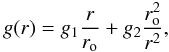 (1)with constants g1 and g2 to allow for both alternatives, which then leads to the following background temperature profile (see also Jones et al. 2011; Gastine & Wicht 2012)
 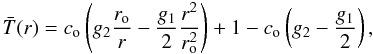 (2)with
 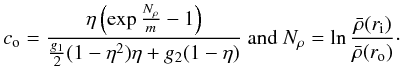 (3)Here, η = ri/ro is the aspect ratio of the spherical shell and Nρ is the number of density scale heights covered by the density background.
Under the anelastic approximation the dimensionless equations that govern convective motions and magnetic field generation are then given by 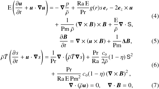 where u, B, p and s are velocity, magnetic field, pressure, and entropy disturbance of the background state, respectively. S is the traceless rate-of-strain tensor with a constant kinematic viscosity given by
  (8)where δij is the identity matrix. In addition to the aspect ratio of the spherical shell η and the two parameters involved in the description of the reference state (Nρ and m), the system of Eqs. (4) − (7) is governed by four dimensionless parameters, namely the Ekman number E, the Prandtl number Pr, the magnetic Prandtl number Pm, and the Rayleigh number Ra defined by
  (9)where gtop is the reference gravity at the outer boundary ro.
2.2. The numerical method
The numerical simulations in this parameter study were computed with the anelastic version of the code MagIC (Wicht 2002; Gastine & Wicht 2012), which has been validated in an anelastic dynamo benchmark (Jones et al. 2011). To solve the system of Eqs. (4) − (7),  and B are decomposed into poloidal and toroidal contributions
  (10)The unknowns W, Z, A, C, s and p are then expanded in spherical harmonic functions up to degree ℓmax in colatitude θ and longitude φ and in Chebyshev polynomials up to degree Nr in the radial direction. An exhaustive description of the complete numerical method and the associated spectral transforms can be found in Gilman & Glatzmaier (1981). Typical numerical resolutions employed in this study range from (Nr = 61, ℓmax = 85) for Boussinesq simulations close to onset to (Nr = 81, ℓmax = 133) for the more demanding cases with a significant density contrast.
In all simulations presented in this study, we assumed constant entropy boundary conditions at ri and ro. The mechanical boundary conditions are either no slip at the inner and stress-free at the outer boundary or stress-free at both limits (see Table 2). The magnetic field matches a potential field at both boundaries.
2.3. Nondimensional diagnostic parameters
To quantify the impact of the different control parameters on magnetic field and flow, we analyse several diagnostic nondimensional properties. The typical rms flow amplitude in the shell is either given as the magnetic Reynolds number Rm = urmsd/λ or as the Rossby number Ro = urms/Ωd. Rm is a measure for the ratio of magnetic field generation to Ohmic dissipation and therefore an important quantity for any dynamo. The Rossby number quantifies the ratio between inertia and Coriolis forces, but Christensen & Aubert (2006) demonstrated that the local Rossby number Roℓ = urms/Ωℓ is a more appropriate measure, at least concerning the impact of inertia on the magnetic field geometry. The typical flow lengthscale ℓ can be calculated based on the spherical harmonic flow contributions  (11)with
  (12)Here, uℓ is the velocity field at a given spherical harmonic degree ℓ and ⟨ ··· ⟩ corresponds to an average over time and radius.
The magnetic field strength can, for example, be measured by the Elsasser number  , which is supposed to provide an estimate for the ratio of Lorentz to Coriolis forces. This estimate may be quite far from the true force balance (e.g. Wicht & Christensen 2010). The modified Elsasser number suggested by Soderlund et al. (2012) and defined by
  (13)provides a more appropriate measure, because it is more directly related to the ratio of the two respective terms in the Navier-Stokes Eq. (4) when approximating the lengthscale that enters the curl in the Lorentz force by
  . In addition to the typical spherical harmonic degree
  , the typical order
  is also used since both seem to contribute (Soderlund et al. 2012):
  (14)Finally, the geometry of the magnetic field is quantified by its dipolarity
  (15)which measures the ratio of the magnetic energy of the dipole to the total magnetic energy at the outer boundary ro.
Critical Rayleigh numbers and corresponding azimuthal wave numbers for the simulations considered in this study (for all of them E = 10-4 and Pr = 1).
2.4. A parameter study
In all simulations presented in this study, the Ekman number is kept fixed to a moderate value of E = 10-4, which allows us to study many different cases. The Prandtl number is set to 1 and the magnetic Prandtl number to 2. Following Jones & Kuzanyan (2009) and our previous hydrodynamical models (Gastine & Wicht 2012), we adopt a polytropic index m = 2 for the reference state. We consider two different aspect ratios: thick shells with η = 0.2 and thin shells with η = 0.6. Dynamo models in thin shells rely on the same setup as our previous hydrodynamical study (Gastine & Wicht 2012). Gravity is adapted to better reflect the different shells, i.e. we use linear gravity in the thick shells (g1 = 1, g2 = 0) and g ∝ 1/r2 in the thin shells (g1 = 0, g2 = 1). Both cases also differ in the flow boundary conditions: thin shell cases assume stress-free conditions at both boundaries, thick shell cases assume a rigid inner boundary.
Because we are mostly interested in the effects of the density stratification, we have performed numerical simulations with different density contrasts spanning the range from Nρ = 0 (i.e. Boussinesq) to Nρ = 3 (i.e. ρbot/ρtop ≃ 20). For each density stratification, we vary the Rayleigh number from simulations close to onset of dynamo action to 10 − 50 times the critical Rayleigh number Rac for the onset of convection. Rac varies with Nρ and we list respective values for the cases explored here in Table 1. These have been determined with the anelastic linear stability analysis code developed by Jones et al. (2009).
As we show below, we find several cases of bistability where a strong dipole-dominated and a weak multipolar solution coexist at identical parameters. The starting solution for our time integration then determines which of the two solutions the simulation will assume. Most of the numerical simulations therefore have been initiated with both a strong dipolar magnetic field (with Λ ~ 1) and a weak multipolar magnetic field (model names end with a “d” or a “m” accordingly in Table 2). Altogether, more than 100 simulations have been computed, each running several magnetic diffusion times to ensure that a stable magnetic configuration has been reached. Table 2 lists the input parameters of all cases along with key solution properties.
3. Results
3.1. Dynamo regimes
Figure 1 shows how the dipolarity fdip depends on the local Rossby number in the thick shell (top) and the thin shell (bottom) simulations. In both geometries we find two distinct branches: The upper branch corresponds to the dipolar regime at fdip > 0.5 with strong magnetic fields at modified Elsasser numbers between Λℓ = 0.1 and Λℓ = 1. This indicates a strong Lorentz force so that these dynamos likely operate in the so-called magnetostrophic regime where Coriolis forces, pressure gradients, buoyancy, and Lorentz forces contribute to the first-order Navier-Stokes equation. In contrast, the models belonging
Results table.
to the lower branch have a multipolar field geometry at fdip < 0.2 and a much weaker magnetic field with Λℓ ≲ 5 × 10⁻². Since the Lorentz force may therefore not enter the first-order Navier-Stokes equation, these cases are likely geostrophic.
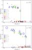 |
Fig. 1 Relative dipole strength plotted against the local Rossby number Roℓ for two different aspect ratios: η = 0.2 (upper panel) and η = 0.6 (lower panel). Each type of symbol is associated to a specific density stratification (from Boussinesq, i.e. Nρ = 0 to stratified simulations corresponding to Nρ = 3). The size of the symbol was chosen according to the value of the modified Elsasser number (Eq. (13)). Vertical lines are tentative transitions between dipolar and multipolar dynamos. |
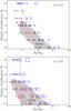 |
Fig. 2 Regime diagram for dynamo simulations as a function of supercriticality and density stratification for two different aspect ratios: η = 0.2 (upper panel) and η = 0.6 (lower panel). Red circles correspond to dipolar dynamos, blue squares to multipolar dynamos, and black crosses are decaying dynamos. The size of the symbols depends on the value of the modified Elsasser number (Eq. (13)). The grey-shaded area highlights the dipolar region, while the dashed lines correspond to the critical Roℓc values that mark the limit between dipolar and multipolar dynamos (see the vertical lines in Fig. 1). |
For both aspect ratios, the dipolar branch is bounded by a critical local Rossby number Roℓc beyond which all cases are multipolar. In the thin shell with η = 0.6, the value Roℓc ≃ 0.15 is slightly higher than the value of Roℓc ≃ 0.12 predicted by Christensen & Aubert (2006) in their geodynamo models with η = 0.35. In the thick shell with η = 0.2, it is lower at Roℓc ≃ 0.08. The critical local Rossby number thus seems to increase with the inner core size. A similar dependence on the aspect ratio has already been found by Aubert et al. (2009). In contrast to the previous Boussinesq studies that used rigid boundary conditions (e.g. Christensen & Aubert 2006; Aubert et al. 2009), the multipolar branch also extends here below the critical Roℓc where the dipolar and the multipolar branch now coexist. This multipolar dynamo branch for Roℓ < 0.1 has also been found in the Boussinesq models of Schrinner et al. (2012) with stress-free boundary conditions. We discuss the bistability phenomenon in more details in Sect. 3.2.
Figure 2 illustrates how the field morphology depends on the stratification and on the supercriticality Ra/Rac. The value Nρ ≃ 1.8 marks an important regime boundary: below this value most cases are bistable (nested circles and squares), while above this value only multipolar cases remain (squares only). The reason for this boundary is considered in Sect. 3.3. The dashed black lines in Fig. 2 mark the Roℓc boundary, which moves to lower supercriticalities for increasing density stratifications. Higher stratifications promote larger flow amplitudes as well as smaller lengthscales since convection is progressively concentrated in a narrowing region close to the outer boundary (see Table 1, Fig. 9 and Jones & Kuzanyan 2009; Gastine & Wicht 2012). Both effects lead to higher Roℓ for a given supercriticality.
For Nρ < 1.8 the boundary for the onset of dynamo action also seems to move to lower supercriticalities when Nρ increases. The reason is a mixture of a decreasing critical magnetic Reynolds number and an increasing flow amplitude for a given supercriticality. Beyond Nρ = 1.8, the critical magnetic Reynolds number once more increases and the onset of dynamo action moves to higher supercriticalities. The onset of dynamo action and the Roℓc boundary are less affected by the stratification for the thinner shell. One reason may be that the flow lengthscale is already quite small for thinner shells even in the Boussinesq case (see Table 1 and Al-Shamali et al. 2004). The differences in the gravity profile and the flow boundary condition may also play a role here.
The dipolar branch reaches down to lower local Rossby numbers than the multipolar branch (see Fig. 1). This is where we find examples of subcritical dynamo action (models 1d, 6d and 12d in Table 2), where the dynamo is only successful when started with a sizable magnetic field strength (Morin & Dormy 2009). Simulations started with a weak field do not have the option to run to the multipolar branch and the field simply decays away.
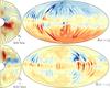 |
Fig. 3 Left panels: isocontours of axisymmetric azimuthal field and poloidal field lines. Right panels: surface radial field Br(r = ro). From a model with η = 0.2, Nρ = 1.7, Ra = 9 × 10⁶ initiated with a dipolar magnetic field (upper panels) and a multipolar one (lower panels). Red (blue) corresponds to positive (negative) values. |
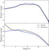 |
Fig. 4 Time-averaged kinetic and magnetic energy spectra plotted against the spherical harmonic degree ℓ. From a model with η = 0.2, Nρ = 1.7, Ra = 9 × 10⁶ initiated with a dipolar magnetic field (black lines) and a multipolar one (blue lines), corresponding to Fig. 3. |
3.2. Bistability
As illustrated in Fig. 2, most of our models at Nρ < 1.8 show bistability. Exceptions are the subcritical thick shell cases and models 13d/m and 14d/m (see Table 2), where even weak initial magnetic fields developed to strong dipoles. The top panel of Fig. 3 shows the dipole-dominated solution with, however, stronger dynamo action in the southern hemisphere. The lower panel of Fig. 3 illustrates the weak multipolar solution, which has pronounced equatorially symmetric and nonaxisymmetric components (this is a feature also visible in the more stratified cases shown in the following Figs. 7, 8). The dipolar solution has a three times larger modified Elsasser number. Generally, Λℓ is twice to ten times larger in the dipole-dominated than in the multipolar counterpart of bistable cases (see Fig. 1 and Table 2 for more details). This suggests that the two dynamo branches are also characterised by different force balances, at least in the bistability region (i.e. Roℓ < 0.1): the dipolar branch is magnetostrophic, while the multipolar one is more likely to be geostrophic. Beyond Roℓ > 0.1, however, the multipolar dynamos can be strong enough to yield a magnetostrophic force balance due to the larger Rayleigh numbers (Brun et al. 2005).
Figure 4 shows the corresponding time-averaged kinetic and magnetic spectra for the two bistable solutions displayed in Fig. 3. The two kinetic energy spectra nearly coincide, emphasising the similarities of the flow in the two solutions. We observe a broad plateau for degrees 4 ≤ ℓ ≤ 30 that reflects the convective driving (for this model, the critical azimuthal wavenumber at onset of convection is m = 6, see Table 1). The magnetic spectra show the differences already visible in the surface magnetic fields displayed in Fig. 3. The amplitude of the dipolar component is more than one order of magnitude lower, higher-order components drop by roughly 50%. A mild maximum for ℓ = 4 corresponds to the large-scale contribution visible in Fig. 3. For spherical harmonic degrees ℓ > 30, the spectra follow some clear power-law behaviour. Both magnetic and kinetic energy spectra have a steep decrease (between ℓ-4 and ℓ-5), very similar to previous stellar dynamo models (e.g. Brun et al. 2005; Browning 2008) or quasi-geostrophic kinematic dynamos (e.g. Schaeffer & Cardin 2006).
The coexistence of a dipolar and a multipolar branch has already been reported for Boussinesq models with stress-free (Busse & Simitev 2006; Schrinner et al. 2012) or mixed mechanical boundary conditions (Sasaki et al. 2011). For rigid boundary conditions only one such case has been found by Christensen & Aubert (2006). Stress-free boundaries allow stronger zonal winds to develop, which seem to play a key role here. These geostrophic flows (constant on coaxial cylinders) are maintained by Reynolds stresses, i.e. by the correlation between the zonal uφ and the cylindrically radial us velocity components (e.g. Gastine & Wicht 2012). For stress-free boundary conditions their amplitude is limited by the weak bulk viscosity. When rigid boundary conditions are employed, the much stronger boundary friction severely brakes these zonal winds.
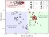 |
Fig. 5 Relative dipole strength plotted against the ratio of axisymmetric toroidal kinetic energy divided by toroidal energy. Red (grey) symbols correspond to simulations in thick (thin) shells (η = 0.2 and η = 0.6, respectively). Each type of symbol is associated with a specific density stratification (from Boussinesq, i.e. Nρ = 0 to Nρ = 3). The sizes of the symbols were chosen according to the values of the modified Elsasser number (Eq. (13)). |
Figure 5 displays the dipolarity of the surface field against the ratio of axisymmetric toroidal to total toroidal kinetic energy, which is a good proxy of the relative amplitude of zonal winds. Strongly dipolar solutions cluster in the upper left corner where zonal winds are weak. For strong zonal winds only weak multipolar solutions can be found. For bistable cases, one solution belongs to the first type while the other one belongs to the second category. There clearly is a competition between strong zonal winds and strong dipolar magnetic fields. The third type of multipolar and sometimes strong solutions with mostly weak zonal winds are mainly strongly stratified cases that we discuss in Sect. 3.3. The strong multipolar fields can have a strong impact on the zonal flows, in a similar way to the stellar models of Brun et al. (2005).
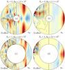 |
Fig. 6 Role of the Ω-effect in the production of the toroidal field for two selected simulations in thick shells (upper panels) and in thin shells (lower panel). For each simulation, the Ω-effect (colour levels) and the axisymmetric azimuthal field (solid and dashed lines) are displayed on the left part, while the axisymmetric zonal flow is given on the right part. Red (blue) corresponds to positive (negative) values. |
The stronger zonal winds in the multipolar cases go along with a change in dynamo mechanism, which is illustrated in Fig. 6. In the dipolar cases (left panels), zonal flows are weak and mainly driven by thermal wind effects. The stronger Lorentz force can balance the Coriolis force and causes these strongly nongeostrophic motions (Aubert 2005). The Ω-effect, i.e. the production of axisymmetric toroidal magnetic field by zonal wind shear, plays only a secondary role (left half of left panels in Fig. 6) so that the dynamo is of the α2 type in the mean field nomenclature (Olson et al. 1999), similar to the planetary dynamo models by Christensen & Aubert (2006) or mean-field models of fully convective stars (Chabrier & Küker 2006). In the multipolar cases (right panels in Fig. 6), significant zonal winds driven by Reynolds stresses develop close to the outer boundary and the associated Ω-effect plays an important role for toroidal magnetic field production. Dynamos on the multipolar branch (for Nρ < 2) are thus of the αΩ or α2Ω type. Many of these solutions show distinct oscillations connected to Parker dynamo waves that we discuss in greater details in Sect. 3.4.
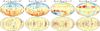 |
Fig. 7 Surface radial field Br(r = ro) (upper panels) and radial velocity close to the outer boundary ur(r = 0.9 ro) (lower panels) for four numerical simulations in thick shells (i.e. η = 0.2) with similar local Rossby number Roℓ ≃ 0.04 − 0.05 (see Table 2). Red (blue) corresponds to positive (negative) values. |
 |
Fig. 8 Surface radial field Br(r = ro) (upper panels) and radial velocity close to the outer boundary ur(r = 0.9 ro) (lower panels) for four numerical simulations in thin shells (i.e. η = 0.6) with similar local Rossby number Roℓ ≃ 0.07−0.08 (see Table 2). Red (blue) corresponds to positive (negative) values. |
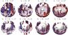 |
Fig. 9 Isocontours and equatorial cut of vorticity along the axis of rotation ωz = (∇ × u)z for different density stratification in thick shells (η = 0.2, upper panels) and in thin shells (η = 0.6, lower panels). These models correspond to the cases displayed in Figs. 7, 8. Positive (negative) values are rendered in red (blue). For each model, the white sphere corresponds to the inner radius. |
3.3. Influence of stratification
For Nρ > 1.8 only the multipolar branch remains. Figures 7 and 8 illustrate how the convective flow and the surface magnetic field evolve on increasing the density stratification for simulations with very similar local Rossby numbers. All these models were initiated with a strong dipolar field. For both aspect ratios, the weakly stratified cases (i.e. Boussinesq and Nρ = 1) have a dipole-dominated magnetic field, while the stronger stratified cases (i.e. Nρ = 2 and Nρ = 3) have multipolar fields with significant nonaxisymmetric contributions. As a consequence of the background density contrast, the typical lengthscale of convection gradually decreases with Nρ (see also Table 1 and Gastine & Wicht 2012). While the imprints of these smaller convective scales are visible in the surface magnetic fields, the dynamos are always dominated by larger scale features even in the strongly stratified cases. For example, for the two models at Nρ = 3, a clear wave number m = 2 signature emerges similar to the patterns already observed in the Boussinesq models of Goudard & Dormy (2008). This magnetic mode can only be clearly identified for moderate magnetic Reynolds numbers Rm < 200 close to the onset of dynamo action. For larger Rm, smaller scale more complex features once more take over.
Some models also show a stronger concentration of the magnetic field in one hemisphere. Similar effects can be found for some multipolar simulations at low stratifications (see Sect. 3.4). Grote & Busse (2000) and Busse & Simitev (2006) reported that hemispherical dynamo action is typical for simulations with stress-free boundaries and Prandtl numbers of about unity.
The collapse of the dipolar branch for Nρ ≳ 2 is caused by the strong concentration of convective features close to the outer boundary where density decreases most drastically. Figure 9 illustrates the evolution of the convective columns when Nρ increases while the local Rossby numbers remains similar (see Figs. 7, 8 for the corresponding magnetic fields and radial flow structures). As has already been demonstrated by nonmagnetic simulations (Jones et al. 2009; Gastine & Wicht 2012), convection first develops close to the inner boundary for Boussinesq and weakly stratified models (Nρ ≤ 1). When increasing Nρ, however, the convective columns gradually move outward and become confined to a thin region close to the equator (Nρ ≥ 2). This goes along with a decrease of the typical lengthscale (see also Table 1 for the critical azimuthal wave numbers at onset). According to Gastine & Wicht (2012), this is a consequence of the fact that buoyancy and thus the effective local Rayleigh number becomes much larger at the outer boundary than in the interior for strongly stratified models.
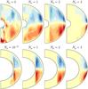 |
Fig. 10 Azimuthal average of kinetic helicity |

The kinetic helicity  is a key ingredient in the induction process via the α-effect (e.g. Moffatt 1978). Figure 10 illustrates how the helicity increasingly concentrates closer to the outer boundary equator when the stratification intensifies simply because the convective columns are the main carriers of helicity. Mean-field dynamo models have demonstrated that a similar concentration of the α-effect can promote nonaxisymmetric dynamo modes of low spherical harmonic order (typically m ~ 1−2, see Rüdiger et al. 2003; Jiang & Wang 2006). Nonaxisymmetric α2Ω mean-field models also suggest a lower critical dynamo number for nonaxisymmetric dynamo modes (e.g. Ruzmaikin et al. 1988; Bassom et al. 2005). These findings may explain the onset of the new larger wave number magnetic mode in our strongly stratified cases.
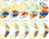 |
Fig. 11 Time evolution of the axisymmetric toroidal magnetic field |

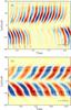 |
Fig. 12 Butterfly diagrams: time evolution of the axisymmetric toroidal magnetic field |
3.4. Parker waves
The αΩ or α2Ω dynamos on the multipolar branch also show a distinct and interesting oscillatory time dependence. Figures 11, 12 illustrate two examples. The magnetic field is weak, multipolar, and dominated by nonaxisymmetric components in both cases (see for example Figs. 7, 8). For the thin shell (lower panels), a dipolar solution coexists at identical parameters. The toroidal magnetic field first emerges at low latitudes, then travels towards the poles and finally vanishes roughly where the tangent cylinder seems to prevent a further movement towards even higher latitudes (Schrinner et al. 2011). When the patches have travelled half way, the cycle starts over with fields of opposite polarity appearing close to the equatorial plane. The thick shell solution (top panels) demonstrates that during some periods one hemisphere clearly dominates. The characteristic period is roughly 0.1 τλ − 0.2τλ, where τλ = d2/λ is the magnetic diffusion time. These are Parker dynamo waves, as we demonstrate below, very similar to those that have been previously identified in some Boussinesq simulations (Goudard & Dormy 2008; Schrinner et al. 2011; Simitev & Busse 2012).
These coherent oscillations lead to the periodic patterns observed in the “butterfly-diagram” style illustrations shown in Fig. 12. The diagrams highlight the direction of travel that in Parker waves is controlled by the gradient of zonal flows: they travel polewards when like in our simulations the differential rotation decreases with depth (e.g. Yoshimura 1975).
The mean-field formalism allows one to derive a dispersion relation for these dynamo waves (Busse & Simitev 2006; Schrinner et al. 2011). In this formalism, magnetic field and flow are decomposed into the axisymmetric or mean contributions denoted by overbars  (16)and the primed nonaxisymmetric or fluctuating contributions B′ and u′. This allows us to reformulate the axisymmetric part of the induction Eq. (5) to
 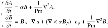 (17)where the fluctuating mean electromotive force is approximated by an α-effect, i.e. by
  .
.
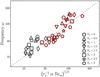 |
Fig. 13 Frequencies of oscillatory dynamos plotted against the dispersion relation of Parker waves given in Eq. (22). Red (grey) symbols correspond to simulations in thick (thin) shells (η = 0.2 and η = 0.6, respectively). Each type of symbol is associated to a specific density stratification. |
To simplify this system, we assume a homogeneous α and also adopt the plane layer formalism introduced by Parker (1955), where the Cartesian coordinates (x,y,z) correspond to (φ,θ,r). Furthermore assuming that  depends only on z (radius) leads to
 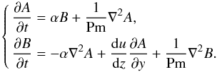 (18)The ansatz A,B ∝ exp(i(kyy + kzz) + λt) with λ = τ + iω allows one to derive the following dispersion relation
  (19)For the αΩ dynamos we concentrated on in the following, the imaginary part of λ provides
  (20)To additionally simplify this dispersion relation, we assume that z variations are of the order of the shell radius, i.e. ky ~ 1/ro and that the shear can be approximated by
  .
.
The α is particularly difficult to estimate. A full derivation of the α tensor would, for example, require to employ the test-field method (e.g. Schrinner et al. 2007). For homogeneous and isotropic MHD turbulence, however, it may at least crudely be approximated via the fluctuating kinetic helicity:  (21)where τc is the typical lifetime of a convective feature (e.g. Brandenburg & Subramanian 2005). Following Brown et al. (2010), we use τc = Hρ/u′ when the local density scale height
  is lower than d and τc = d/u′ otherwise. This finally leads to the simplified dispersion relation for Parker waves
  (22)Figure 13 shows the comparison between the frequencies predicted by this simplified dispersion relation and those found in the numerical models. The latter frequencies are obtained using a Fourier transform of the butterfly diagrams displayed in Fig. 12. The resulting
  is then integrated over the colatitude θ to derive the power spectrum. Even though individual predictions fail by up to a factor two, the general agreement is quite convincing given the numerous approximation involved and is similar to that reached in previous Boussinesq studies (Busse & Simitev 2006; Schrinner et al. 2011). This confirms that the oscillations in our multipolar cases are indeed Parker waves. When the magnetic Reynolds number becomes too large (Rm ≳ 150 − 200), the coherence of these oscillations is gradually lost and a definite frequency is increasingly difficult to determine. This limits our analysis to lower Rezon and α values and to frequencies ω < 300.
4. Discussion and conclusions
We have investigated the influence of background density stratification on convection-driven dynamos in a rotating spherical shell. The use of the anelastic approximation allowed us to exclude sound waves and the related short time steps (Gilman & Glatzmaier 1981; Clune et al. 1999; Jones & Kuzanyan 2009). Previous Boussinesq results have shown that inertial effects play a decisive role for determining the magnetic field geometry. When inertia becomes influential, only multipolar solutions with weak magnetic fields are possible. When inertia is weak, two solutions can coexist: dipole-dominated solutions with strong magnetic fields are found for stress-free as well as rigid boundary conditions. For stress-free and mixed boundary conditions, a multipolar branch is found at identical parameters (e.g. Simitev & Busse 2009; Schrinner et al. 2012). Alternatively, the recent study by Soderlund et al. (2012) suggests that the transition between dipolar and multipolar dynamos may occur when inertia becomes higher than viscous forces. This transition is accompanied by an abrupt decrease of the kinetic helicity. However, these results seem to be in contradiction with previous studies where inertia is always higher than viscosity (e.g. Wicht & Christensen 2010) and more investigations are required to clarify this contradiction.
Our anelastic simulations confirm this scenario for mild stratifications corresponding to Nρ < 1.8. The reason for the bistability is a competition between zonal winds and dipolar magnetic fields. Strong dipolar magnetic fields prevent significant zonal winds from developing. Strong zonal winds, on the other hand, prevent the production of significant dipolar fields. The two branches also differ in the induction mechanism. Strong zonal winds promote an Ω-effect, which leads to a αΩ or α2Ω type of dynamo, while dipole-dominated magnetic fields are typically generated in an α2 process. The sizable axisymmetric toroidal fields produced by an Ω-effect typically lead to a coherent cyclic time evolution of the magnetic field for moderate magnetic Reynolds numbers (Rm < 200). This is consistent with previous Boussinesq studies (e.g. Schrinner et al. 2007) and numerical models of young solar-type stars (Brown et al. 2011) and has been identified as Parker waves. In contrast to what is observed in the solar cycle, these waves start at the equator and travel towards the poles because of the opposite sign in the zonal shear.
For stronger stratification with Nρ > 1.8, the dipolar branch is lost and close to the onset of dynamo action a new magnetic mode characterised by a large wave number m = 2 appears. This is likely due to the concentration of the α-effect into a narrow region close to the equator. According to mean-field models, this would preferentially promote nonaxisymmetric dynamos (see also Chabrier & Küker 2006) with large wave numbers. The collapse of the dipolar branch may explain the differences between the weakly stratified and significantly dipolar simulations by Dobler et al. (2006) (ρbot/ρtop ≃ 5, i.e. Nρ = 1.6) and the strongly stratified anelastic and multipolar models by Browning (2008) (ρbot/ρtop ≃ 100, i.e. Nρ = 4.6).
Numerical limitations force us to use excessively high diffusivities in our simulations. Ekman numbers are thus orders of magnitude too large and Reynolds number orders of magnitude too low. When extrapolated to fast-rotating planets and stars, this type of models nevertheless provides, for example, realistic magnetic field strengths (Olson & Christensen 2006; Christensen et al. 2009). This gives us confidence to compare the observed field geometries of planets and stars with predictions based on our simulation results.
Our results are compatible with the dipole-dominated magnetic fields on Jupiter and Saturn that are generated in their deeper metallic envelopes where the density stratification is only mild (roughly Nρ ~ 1.5 − 2, see Heimpel & Gómez Pérez 2011; Nettelmann et al. 2012). Since the local Rossby number is very small for these planets, however, bistability seems to be an option. This is also the case for Uranus and Neptune, where Roℓ and the density contrast within the dynamo region are small (Hubbard et al. 1991; Olson & Christensen 2006). Their multipolar magnetic field would then suggest that these planets would then occupy the alternative branch offered by the bistability phenomenon.
Concerning rapidly rotating low-mass stars that may also fall into the low Roℓ regime, the spectropolarimetric observations of Morin et al. (2010) suggest that late M stars with very similar parameters (mass and rotation rate) fall into two categories: some stars present a strong dipole-dominated magnetic field while others show weaker and multipolar magnetic structures. These two geometries may represent the two coexisting dynamo branches at smaller local Rossby numbers.
For the bistability to be a viable explanation, however, our simulations suggest that the dynamos must operate in a region with moderate density stratification (Nρ ~ 1 − 2) and supercriticality (Ra/Rac ~ 10 − 30). Since the stellar dynamos presumably operate far from the onset of convection, only multipolar fields would be possible. However, when decreasing the Ekman number towards more realistic values, the simulations by Christensen & Aubert (2006) suggest that the dipolar window may persist at higher supercriticalities. In addition, since these stars have a huge density contrast, our investigation would generally predict multipolar fields. Additional exploration of the parameter space seems required here to clarify this point. Stanley & Glatzmaier (2010), for example, suggested that lower Prandtl numbers may help in creating stronger dipole fields. Radial-dependent properties (e.g. viscosity, thermal diffusivity and electrical diffusivity) are also known to have a strong impact on the location of the convective columns that could possibly help to avoid the concentration of helicity close to the equator.
Acknowledgments
All computations were carried out on the GWDG computer facilities in Göttingen. This work was supported by the Special Priority Program 1488 (PlanetMag, http://www.planetmag.de) of the German Science Foundation. It is a pleasure to thank C. A. Jones for providing us his linear stability code.
References
- Al-Shamali, F. M., Heimpel, M. H., & Aurnou, J. M. 2004, Geophys. Astrophys. Fluid Dyn., 98, 153 [NASA ADS] [CrossRef] [Google Scholar]
- Aubert, J. 2005, J. Fluid Mech., 542, 53 [NASA ADS] [CrossRef] [Google Scholar]
- Aubert, J., Labrosse, S., & Poitou, C. 2009, Geophys. J. Int., 179, 1414 [NASA ADS] [CrossRef] [Google Scholar]
- Bassom, A. P., Kuzanyan, K. M., Sokoloff, D., & Soward, A. M. 2005, Geophys. Astrophys. Fluid Dyn., 99, 309 [NASA ADS] [CrossRef] [Google Scholar]
- Bessolaz, N., & Brun, A. S. 2011, Astron. Nachr., 332, 1045 [NASA ADS] [CrossRef] [Google Scholar]
- Braginsky, S. I., & Roberts, P. H. 1995, Geophys. Astrophys. Fluid Dyn., 79, 1 [NASA ADS] [CrossRef] [Google Scholar]
- Brandenburg, A., & Subramanian, K. 2005, Phys. Rep., 417, 1 [NASA ADS] [CrossRef] [Google Scholar]
- Brown, B. P., Browning, M. K., Brun, A. S., Miesch, M. S., & Toomre, J. 2010, ApJ, 711, 424 [Google Scholar]
- Brown, B. P., Miesch, M. S., Browning, M. K., Brun, A. S., & Toomre, J. 2011, ApJ, 731, 69 [NASA ADS] [CrossRef] [Google Scholar]
- Browning, M. K. 2008, ApJ, 676, 1262 [Google Scholar]
- Brun, A. S., Browning, M. K., & Toomre, J. 2005, ApJ, 629, 461 [NASA ADS] [CrossRef] [Google Scholar]
- Busse, F. H., & Simitev, R. D. 2006, Geophys. Astrophys. Fluid Dyn., 100, 341 [NASA ADS] [CrossRef] [Google Scholar]
- Chabrier, G., & Küker, M. 2006, A&A, 446, 1027 [NASA ADS] [CrossRef] [EDP Sciences] [Google Scholar]
- Christensen, U. R. 2006, Nature, 444, 1056 [NASA ADS] [CrossRef] [Google Scholar]
- Christensen, U. R. 2010, Space Sci. Rev., 152, 565 [NASA ADS] [CrossRef] [Google Scholar]
- Christensen, U. R., & Aubert, J. 2006, Geophys. J. Int., 166, 97 [NASA ADS] [CrossRef] [Google Scholar]
- Christensen, U. R., Holzwarth, V., & Reiners, A. 2009, Nature, 457, 167 [NASA ADS] [CrossRef] [PubMed] [Google Scholar]
- Clune, T. C., Elliott, J. R., Miesch, M. S., Toomre, J., & Glatzmaier, G. A. 1999, Parallel Computing, 25, 361 [Google Scholar]
- Dobler, W., Stix, M., & Brandenburg, A. 2006, ApJ, 638, 336 [NASA ADS] [CrossRef] [Google Scholar]
- Donati, J., Forveille, T., Cameron, A. C., et al. 2006, Science, 311, 633 [NASA ADS] [CrossRef] [PubMed] [Google Scholar]
- Donati, J., Morin, J., Petit, P., et al. 2008, MNRAS, 390, 545 [NASA ADS] [CrossRef] [Google Scholar]
- Gastine, T., & Wicht, J. 2012, Icarus, 219, 428 [NASA ADS] [CrossRef] [Google Scholar]
- Gilman, P. A., & Glatzmaier, G. A. 1981, ApJS, 45, 335 [NASA ADS] [CrossRef] [Google Scholar]
- Glatzmaier, G. A. 1984, J. Comput. Phys., 55, 461 [Google Scholar]
- Goudard, L., & Dormy, E. 2008, Europhys. Lett., 83, 59001 [NASA ADS] [CrossRef] [EDP Sciences] [Google Scholar]
- Grote, E., & Busse, F. H. 2000, Phys. Rev. E, 62, 4457 [Google Scholar]
- Heimpel, M., & Gómez Pérez, N. 2011, Geophys. Res. Lett., 38, L14201 [NASA ADS] [CrossRef] [Google Scholar]
- Hubbard, W. B., Nellis, W. J., Mitchell, A. C., et al. 1991, Science, 253, 648 [NASA ADS] [CrossRef] [Google Scholar]
- Jiang, J., & Wang, J.-X. 2006, Chinese J. Astron. Astrophys., 6, 227 [Google Scholar]
- Jones, C. A., & Kuzanyan, K. M. 2009, Icarus, 204, 227 [NASA ADS] [CrossRef] [Google Scholar]
- Jones, C. A., Kuzanyan, K. M., & Mitchell, R. H. 2009, J. Fluid Mech., 634, 291 [NASA ADS] [CrossRef] [Google Scholar]
- Jones, C. A., Boronski, P., Brun, A. S., et al. 2011, Icarus, 216, 120 [NASA ADS] [CrossRef] [Google Scholar]
- Kutzner, C., & Christensen, U. R. 2002, Phys. Earth Planet. In., 131, 29 [Google Scholar]
- Lantz, S. R., & Fan, Y. 1999, ApJS, 121, 247 [Google Scholar]
- Moffatt, H. K. 1978, Magnetic field generation in electrically conducting fluids (Cambridge, England: Cambridge University Press), 353 [Google Scholar]
- Morin, V., & Dormy, E. 2009, Int. J. Mod. Phys. B, 23, 5467 [NASA ADS] [CrossRef] [Google Scholar]
- Morin, J., Donati, J., Petit, P., et al. 2008, MNRAS, 390, 567 [NASA ADS] [CrossRef] [MathSciNet] [Google Scholar]
- Morin, J., Donati, J.-F., Petit, P., et al. 2010, MNRAS, 407, 2269 [NASA ADS] [CrossRef] [MathSciNet] [Google Scholar]
- Nettelmann, N., Becker, A., Holst, B., & Redmer, R. 2012, ApJ, 750, 52 [NASA ADS] [CrossRef] [Google Scholar]
- Olson, P., & Christensen, U. R. 2006, Earth Planet. Sci. Lett., 250, 561 [NASA ADS] [CrossRef] [Google Scholar]
- Olson, P., Christensen, U., & Glatzmaier, G. A. 1999, J. Geophys. Res., 104, 10383 [NASA ADS] [CrossRef] [Google Scholar]
- Parker, E. N. 1955, ApJ, 122, 293 [NASA ADS] [CrossRef] [Google Scholar]
- Rüdiger, G., Elstner, D., & Ossendrijver, M. 2003, A&A, 406, 15 [NASA ADS] [CrossRef] [EDP Sciences] [Google Scholar]
- Ruzmaikin, A. A., Sokolov, D. D., & Starchenko, S. V. 1988, Sol. Phys., 115, 5 [NASA ADS] [CrossRef] [Google Scholar]
- Sasaki, Y., Takehiro, S.-I., Kuramoto, K., & Hayashi, Y.-Y. 2011, Phys. Earth Planet. Int., 188, 203 [Google Scholar]
- Schaeffer, N., & Cardin, P. 2006, Earth Planet. Sci. Lett., 245, 595 [NASA ADS] [CrossRef] [Google Scholar]
- Schrinner, M., Rädler, K.-H., Schmitt, D., Rheinhardt, M., & Christensen, U. R. 2007, Geophys. Astrophys. Fluid Dyn., 101, 81 [NASA ADS] [CrossRef] [MathSciNet] [Google Scholar]
- Schrinner, M., Petitdemange, L., & Dormy, E. 2011, A&A, 530, A140 [NASA ADS] [CrossRef] [EDP Sciences] [Google Scholar]
- Schrinner, M., Petitdemange, L., & Dormy, E. 2012, ApJ, 752, 121 [NASA ADS] [CrossRef] [Google Scholar]
- Simitev, R. D., & Busse, F. H. 2009, Europhys. Lett., 85, 19001 [NASA ADS] [CrossRef] [EDP Sciences] [Google Scholar]
- Simitev, R. D., & Busse, F. H. 2012, ApJ, 749, 9 [NASA ADS] [CrossRef] [Google Scholar]
- Soderlund, K. M., King, E. M., & Aurnou, J. M. 2012, Earth Planet. Sci. Lett., 333, 9 [NASA ADS] [CrossRef] [Google Scholar]
- Sreenivasan, B., & Jones, C. A. 2006, Geophys. J. Int., 164, 467 [NASA ADS] [CrossRef] [Google Scholar]
- Stanley, S., & Glatzmaier, G. A. 2010, Space Sci. Rev., 152, 617 [Google Scholar]
- Wicht, J. 2002, Phys. Earth Planet. Int., 132, 281 [CrossRef] [Google Scholar]
- Wicht, J., & Christensen, U. R. 2010, Geophys. J. Int., 181, 1367 [NASA ADS] [Google Scholar]
- Yoshimura, H. 1975, ApJ, 201, 740 [NASA ADS] [CrossRef] [Google Scholar]
All Tables
Critical Rayleigh numbers and corresponding azimuthal wave numbers for the simulations considered in this study (for all of them E = 10-4 and Pr = 1).
All Figures
|
Fig. 1 Relative dipole strength plotted against the local Rossby number Roℓ for two different aspect ratios: η = 0.2 (upper panel) and η = 0.6 (lower panel). Each type of symbol is associated to a specific density stratification (from Boussinesq, i.e. Nρ = 0 to stratified simulations corresponding to Nρ = 3). The size of the symbol was chosen according to the value of the modified Elsasser number (Eq. (13)). Vertical lines are tentative transitions between dipolar and multipolar dynamos. |
| In the text | |
|
Fig. 2 Regime diagram for dynamo simulations as a function of supercriticality and density stratification for two different aspect ratios: η = 0.2 (upper panel) and η = 0.6 (lower panel). Red circles correspond to dipolar dynamos, blue squares to multipolar dynamos, and black crosses are decaying dynamos. The size of the symbols depends on the value of the modified Elsasser number (Eq. (13)). The grey-shaded area highlights the dipolar region, while the dashed lines correspond to the critical Roℓc values that mark the limit between dipolar and multipolar dynamos (see the vertical lines in Fig. 1). |
| In the text | |
|
Fig. 3 Left panels: isocontours of axisymmetric azimuthal field and poloidal field lines. Right panels: surface radial field Br(r = ro). From a model with η = 0.2, Nρ = 1.7, Ra = 9 × 10⁶ initiated with a dipolar magnetic field (upper panels) and a multipolar one (lower panels). Red (blue) corresponds to positive (negative) values. |
| In the text | |
|
Fig. 4 Time-averaged kinetic and magnetic energy spectra plotted against the spherical harmonic degree ℓ. From a model with η = 0.2, Nρ = 1.7, Ra = 9 × 10⁶ initiated with a dipolar magnetic field (black lines) and a multipolar one (blue lines), corresponding to Fig. 3. |
| In the text | |
|
Fig. 5 Relative dipole strength plotted against the ratio of axisymmetric toroidal kinetic energy divided by toroidal energy. Red (grey) symbols correspond to simulations in thick (thin) shells (η = 0.2 and η = 0.6, respectively). Each type of symbol is associated with a specific density stratification (from Boussinesq, i.e. Nρ = 0 to Nρ = 3). The sizes of the symbols were chosen according to the values of the modified Elsasser number (Eq. (13)). |
| In the text | |
|
Fig. 6 Role of the Ω-effect in the production of the toroidal field for two selected simulations in thick shells (upper panels) and in thin shells (lower panel). For each simulation, the Ω-effect (colour levels) and the axisymmetric azimuthal field (solid and dashed lines) are displayed on the left part, while the axisymmetric zonal flow is given on the right part. Red (blue) corresponds to positive (negative) values. |
| In the text | |
|
Fig. 7 Surface radial field Br(r = ro) (upper panels) and radial velocity close to the outer boundary ur(r = 0.9 ro) (lower panels) for four numerical simulations in thick shells (i.e. η = 0.2) with similar local Rossby number Roℓ ≃ 0.04 − 0.05 (see Table 2). Red (blue) corresponds to positive (negative) values. |
| In the text | |
|
Fig. 8 Surface radial field Br(r = ro) (upper panels) and radial velocity close to the outer boundary ur(r = 0.9 ro) (lower panels) for four numerical simulations in thin shells (i.e. η = 0.6) with similar local Rossby number Roℓ ≃ 0.07−0.08 (see Table 2). Red (blue) corresponds to positive (negative) values. |
| In the text | |
|
Fig. 9 Isocontours and equatorial cut of vorticity along the axis of rotation ωz = (∇ × u)z for different density stratification in thick shells (η = 0.2, upper panels) and in thin shells (η = 0.6, lower panels). These models correspond to the cases displayed in Figs. 7, 8. Positive (negative) values are rendered in red (blue). For each model, the white sphere corresponds to the inner radius. |
| In the text | |
|
Fig. 10 Azimuthal average of kinetic helicity |
| In the text | |
|
Fig. 11 Time evolution of the axisymmetric toroidal magnetic field |
| In the text | |
|
Fig. 12 Butterfly diagrams: time evolution of the axisymmetric toroidal magnetic field |
| In the text | |
|
Fig. 13 Frequencies of oscillatory dynamos plotted against the dispersion relation of Parker waves given in Eq. (22). Red (grey) symbols correspond to simulations in thick (thin) shells (η = 0.2 and η = 0.6, respectively). Each type of symbol is associated to a specific density stratification. |
| In the text | |
Current usage metrics show cumulative count of Article Views (full-text article views including HTML views, PDF and ePub downloads, according to the available data) and Abstracts Views on Vision4Press platform.
Data correspond to usage on the plateform after 2015. The current usage metrics is available 48-96 hours after online publication and is updated daily on week days.
Initial download of the metrics may take a while.