| Issue |
A&A
Volume 546, October 2012
|
|
|---|---|---|
| Article Number | A7 | |
| Number of page(s) | 8 | |
| Section | Interstellar and circumstellar matter | |
| DOI | https://doi.org/10.1051/0004-6361/201219336 | |
| Published online | 26 September 2012 | |
DoAr 33: a good candidate for revealing dust growth and settling in protoplanetary disks
1
Purple Mountain Observatory, Chinese Academy of Sciences,
2 West Beijing Road, 210008
Nanjing,
PR China
e-mail: This email address is being protected from spambots. You need JavaScript enabled to view it.
2
Graduate School of the Chinese Academy of Sciences,
100080
Beijing, PR
China
3
Institut für Theoretische Physik und Astrophysik, Universität zu
Kiel, Leibnizstr.
15, 24118
Kiel,
Germany
Received: 3 April 2012
Accepted: 20 August 2012
Abstract
Aims. We aim to evaluate the evolutionary stage of the circumstellar disk around DoAr 33, a T Tauri star in the Ophiuchus molecular cloud and a promising target for follow-up observations to find signs of dust evolution in protoplanetary disks.
Methods. The currently available data on DoAr 33 comprises its spectral energy distribution from the optical to the millimeter regimes. This data set allows us to characterize the structure of a circumstellar disk using self-consistent radiative transfer models. We employed two different types of models, a well-mixed model and a settled disk model in which dust growth and settling are taken into account. Simulated annealing was used to search for an optimum parameter set.
Results. Our results suggest that the assumption of a well-mixed dust and gas phase leads to overestimation of the mid-infrared flux, whereas the (sub)millimeter emission can be predicted quite well. Observational and theoretical arguments imply that an overall decrease in mid-infrared flux can be explained by dust growth and settling towards the midplane of the disk. As expected, the settled disk model is able to satisfactorily reproduce the data points at all wavelengths. DoAr 33 is therefore a good candidate for studying dust growth and settling in protoplanetary disks, so it deserves to be investigated with future observations.
Key words: circumstellar matter / protoplanetary disks / radiative transfer
© ESO, 2012
1. Introduction
Protoplanetary disks are both the birthplace of planets and a necessary evolutionary component of young stellar objects (YSOs). The dust and gas in these disks constitute the building blocks of planets. To date, the most widely accepted planet formation theory is the core accretion-gas capture model (e.g., Pollack et al. 1996; Papaloizou & Terquem 2006; Lissauer & Stevenson 2007). Dust grains coagulate and grow within the disks, settle towards the midplane, and are eventually assembled to larger entities, such as pebbles and planetesimals (e.g., Carballido et al. 2006; Dominik et al. 2007). The gas-phase material dissipates over time by accretion onto the central star, disk winds and jets, and photoevaporation (Alexander et al. 2006; Balog et al. 2008) or can be captured by growing gas-giant and ice-giant planets (e.g., Machida et al. 2010). Dust growth and settling are therefore considered as the key processes in the early phase of planet formation. Studying these effects helps in understanding how planet formation is initiated in disks and which role this process plays in the evolution of circumstellar disks.
Direct evidence for dust growth in protoplanetary disks can be derived from analyzing the spectral energy distributions (SEDs) of YSOs. A population of larger grains increases the emissivity at (sub)millimeter wavelengths and shallows the spectral index in this wavelength domain as compared to the interstellar medium (ISM) (e.g., Beckwith & Sargent 1991; Testi et al. 2001; Natta et al. 2004). Dust growth can also be inferred from the overall level of infrared (IR) flux. Disks with larger dust grains have lower opacities within the stellar spectrum and can thus reprocess less energy, resulting in a cooler temperature distribution and less IR flux (e.g., Bouwman et al. 2008). Moreover, grain growth also influences spectral emission signatures of the dust. For instance, the 10 μm silicate feature widely present in YSOs is produced by small grains and disappears when the size distribution changes towards larger grain radii (e.g., D’Alessio et al. 2001; van Boekel et al. 2005; Kessler-Silacci et al. 2006; Schegerer et al. 2006; Pinte et al. 2008).
Dust settling might be a common feature of protoplanetary disks since observations show that most T Tauri stars exhibit less mid-IR emission than expected for a disk in which dust and gas are well mixed and coupled (e.g., Furlan et al. 2005, 2006). As the central star ages dust grains gradually separate from the gas and settle toward the disk midplane due to the gravity exerted by the central star (e.g., Schräpler & Henning 2004; Nomura & Nakagawa 2006), leading to a reduced flaring angle of the disk and a decrease in IR flux. Mid-IR slopes can therefore be used as a diagnostic for dust settling. This explanation is confirmed by theoretical modeling (e.g., Dullemond & Dominik 2004b; D’Alessio et al. 2006) and an abundant set of observations (e.g., Chiang et al. 2001; Bouwman et al. 2008; Juhász et al. 2010).
This means that SED analysis and modeling work together to act as an effective tool for studying the structure and evolution of protoplanetary disks and can provide a first hint on the progress of dust growth and settling. Consequently, the SED can be used to identify promising objects for subsequent high-resolution observations aimed at studying these processes in YSOs. In this paper we focus on the SED fitting of the object DoAr 33 (α = 16:27:39.0, δ = −23:58:18.3), a T Tauri star located in the Ophiuchus star formation region at a distance of ~125 pc (Loinard et al. 2008). It is one of the 26 transition disks identified by Cieza et al. (2010) based on multiwavelength photometry and high-resolution optical spectroscopy, in their nomenclature TRAN 17. The photometric measurements available for this object are compiled in Fig. 1. DoAr 33 is a class II source (Evans et al. 2009) with its SED flattened around ~70 μm, an unusual feature for typical YSOs at this evolutionary stage (Lada 1999). As dust settling is efficient in steepening the SED at mid- to far-IR wavelengths (Dullemond & Dominik 2004b), this feature makes DoAr 33 very promising for finding signs of disk evolution. The three (sub)millimeter data points from SCUBA, IRAM, and ATCA allow us to place constraints on the dust mass and maximum grain size for a given dust model and also reduce the SED model degeneracy.
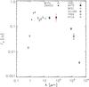 |
Fig. 1 SED data of DoAr 33: WIYN (Wilking et al. 2005), 2MASS, IRAC, and MIPS (Evans et al. 2009), WISE (WISE All Sky Data Release 2012), MIPS upper limit at 70 μm (red triangle, Cieza et al. 2010), SCUBA and IRAM (Andrews et al. 2007), ATCA (Ricci et al. 2010). |
2. Disk model
In this section, we introduce two disk models employed in our study to fit the observed SED of DoAr 33.
2.1. Dust properties
The dust grain properties consist of three parts: the shape of the dust grain, the chemical composition, and the grain size distribution.
-
Grain shape:
We consider the dust grains to be homogeneousspheres. Although real dust grains are expected to have acomplicated and fractal structure, the spherical-shape assumptionis a valid approximation because the scattering behavior is similar,and we do not expect the dust grains to be aligned on a large scale bymagnetic fields.
-
Grain chemistry:
The dust grain ensemble incorporates both silicate and graphite material with relative abundances of 62.5% astronomical silicate and 37.5% graphite. With the Mie scattering theory, we calculate the optical properties of the dust using the complex refractive indices of “smoothed astronomical silicate” and graphite published by Weingartner & Draine (2001).
-
Grain size distribution:
The grain size distribution is given by the power law n(a) ∝ a-3.5 with amin ≤ a ≤ amax, where a represents the grain radius and n(a)da is the number of dust grains with a specific radius in [a, a+da]. The minimum grain size is fixed to amin = 5 nm. We use a very low value for this parameter to ensure that its exact value has a negligible effect on the emergent SED. The maximum grain size amax depends on the dust density distribution of the disk that is described in the following section.
2.2. Dust density distribution
2.2.1. Settled disk scenario
The upper panel of Fig. 2 depicts the configuration of a two-layer parameterized disk that takes the effects of dust settling and growth into account. Similar models have been used to study the impact of dust growth and sedimentation in circumstellar disks on SEDs (D’Alessio et al. 2006) and on multiwavelength images (Sauter & Wolf 2011). The upper layer represents the population of small dust grains that either have not grown or are produced inside the disk and lifted up by turbulent mixing. This population continuously feeds the deeper layer closer to the disk midplane that contains large dust grains. We assume a dust density structure with a Gaussian vertical profile as described by Shakura & Sunyaev (1973): ![Mathematical equation: \begin{equation} \rho_{\rm{dust}} = \rho_{0}\left(\frac{R_{\star}}{R}\right)^{\alpha}\exp\left[-\frac{1}{2}\left(\frac{z}{h(R)}\right)^{2}\right], \end{equation}](/articles/aa/full_html/2012/10/aa19336-12/aa19336-12-eq14.png) (1)where R is the radial distance from the central star measured in the disk midplane, R⋆ the stellar radius, and h(R) the disk scale height for different dust populations calculated by
(1)where R is the radial distance from the central star measured in the disk midplane, R⋆ the stellar radius, and h(R) the disk scale height for different dust populations calculated by ![Mathematical equation: \begin{eqnarray} h_{\rm{small}} &&= h_{100}\left(\frac{R}{100~\rm{AU}}\right)^{\beta} \\[1.5mm] h_{\rm{large}} &&= h_{\rm{small}}/H_{\rm {ratio}}. \end{eqnarray}](/articles/aa/full_html/2012/10/aa19336-12/aa19336-12-eq18.png) The surface density follows a power law Σ(R) = Σ0(R/R⋆)−p with p = α − β. The quantities ρ0 and Σ0 are determined by normalizing the total dust mass in the disk. The exponent β describes the extent of disk flaring. The relative sedimentation height Hratio characterizes the level of turbulence in the disk, and we use h100 = h(100 AU) to adjust the scale height of the small dust population at a given radial distance.
The surface density follows a power law Σ(R) = Σ0(R/R⋆)−p with p = α − β. The quantities ρ0 and Σ0 are determined by normalizing the total dust mass in the disk. The exponent β describes the extent of disk flaring. The relative sedimentation height Hratio characterizes the level of turbulence in the disk, and we use h100 = h(100 AU) to adjust the scale height of the small dust population at a given radial distance.
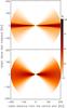 |
Fig. 2 Dust density distribution normalized to the maximum on a plane perpendicular to the disk midplane. For better graphical representation, the fourth root of the function is plotted. Upper plot: disk model with the inclusion of dust settling. Large grains dominate the density in the midplane, while small grains are present everywhere in the disk. Lower plot: well-mixed model in which the grain size distribution is homogeneous at all disk radii. |
As introduced by D’Alessio et al. (2006), two populations of small and large grains with different dust-to-gas ratios are used to simulate grain growth and settling by moving mass from one grain population to the next. The maximum grain size amax is fixed in the upper layer to 0.25 μm and is a free parameter for the large grain population. A parameter  (4)is introduced to quantify the depletion of the small dust grains relative to the standard dust-to-gas ratio found in the ISM, where ζISM = 0.01 and ζsmall is the dust-to-gas mass ratio in the small dust grain population. To calculate the relative weighting factor of the large dust population (ζlarge), we use the approximate relationship
 ![Mathematical equation: \begin{equation} \frac{\zeta_{\rm{large}}}{\zeta_{\rm{ISM}}}=\left[1+\left(\frac{\sqrt{2\pi}}{2\delta}-1\right)\left(1-\frac{\zeta_{\rm{small}}}{\zeta_{\rm{ISM}}}\right)\right], \end{equation}](/articles/aa/full_html/2012/10/aa19336-12/aa19336-12-eq31.png) (5)where we adopt δ = 0.1, see the appendix of D’Alessio et al. (2006). Moreover, the depletion parameter ϵ is assumed to be independent of the radial position in the disk.
(5)where we adopt δ = 0.1, see the appendix of D’Alessio et al. (2006). Moreover, the depletion parameter ϵ is assumed to be independent of the radial position in the disk.
2.2.2. Well-mixed disk scenario
Flared disk models with a homogeneous dust distribution (lower panel of Fig. 2) have been successfully used to interpret multiwavelength observations of YSOs like the SED in our study (e.g., Andrews et al. 2009; Orellana et al. 2012). A well-mixed scenario can be considered as a limiting case of the settled disk model described in the previous section. When the sedimentation height Hratio and the depletion parameter ϵ tend towards 1, and the maximum grain size amax for both grain populations are identical, the settled disk model turns into the well-mixed case.
2.3. Heating sources
Circumstellar disks can generally be divided into two types, active disks and passive disks, depending on the relevance of accretion. The dusty disk can be actively heated by the loss of gravitational energy released from material as it accretes onto the central star (e.g., D’Alessio et al. 1998), which is the so-called accretion heating scheme. This heating mechanism might be important in the early evolutionary stages (e.g., Class 0/I object), since the accretion rate is much higher than more evolved sources. Alternatively, the circumstellar disk can passively re-emit the energy it absorbs from the central star at longer wavelengths (e.g., Chiang & Goldreich 1997).
For our object DoAr 33, we calculate the accretion luminosity using the approximate formula: 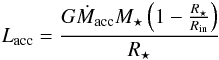 (6)where Rin denotes the truncation radius of the inner disk and is set to be 5 R⋆ (Gullbring et al. 1998). The stellar radius (R⋆) is taken to be 2.12 R⊙ and mass (M⋆) is 1.44 M⊙ (Ricci et al. 2010). The low accretion rate Ṁacc = 2.52 × 10⁻¹⁰ M⊙/yr derived by Cieza et al. (2010) yields an accretion luminosity (0.0043 L⊙) that is only ~0.3% of the blackbody luminosity of the central star (~1.5 L⊙). Furthermore, accretion disk theory shows that only about <50% of this accretion energy contributes to the heating of circumstellar disks (e.g., Calvet & Gullbring 1998). Therefore, we neglect the accretion energy in our simulation, leading to a simple passive disk model.
The spectral type K5.5 of DoAr 33 derived by Wilking et al. (2005) implies an effective temperature of ~4250 K using the SpT − Teff relationship given by Kenyon & Hartmann (1995). The luminosity of the star is considered as a free parameter. The incident stellar spectra is taken from the NextGen atmosphere database with log g = 3.5 and solar metallicity (Hauschildt et al. 1999). SED simulations are performed using the well-tested code MC3D (Wolf 2003). Based on the Monte-Carlo method, the radiative transfer problem is solved self-consistently considering 110 wavelengths, distributed in a logarithmic scale between 0.1 μm and 4000 μm.
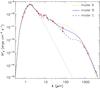 |
Fig. 3 The top three model fits found by SA. The red diamonds depict the photometric measurements and the black arrow represents the upper limit for the 70 μm flux (Cieza et al. 2010). The gray dotted line marks the contribution of the central star to the total flux of the system. |
3. Results and discussion
The SED-fitting task is conducted using simulated annealing (SA) technique (Kirkpatrick et al. 1983), a Markov Chain Monte Carlo method based on the Metropolis-Hastings algorithm (Metropolis et al. 1953; Hastings 1970). A detailed description of this approach can be found in the appendix. We started our parameter study with the simpler well-mixed model. The predicted fluxes of the best-fit model found by SA in the allocated timeframe are overlayed with observed data points in Fig. 3, and the parameter set is listed in Table 1, i.e. model A. In the fitting procedure, the distance to DoAr 33 was fixed to 125 pc and an extinction Av = 4.8 as reported by the Spitzer/c2d program (Evans et al. 2009) was taken to correct the fluxes with the extinction law of Cardelli et al. (1989) and Rv = 3.1. In any case, the extinction is only appreciable for wavelengths ≲5 μm. The model predictions exceed the observations in the mid-IR, most notably the MIPS data point at 70 μm given by Evans et al. (2009), nearly three-fold. For the upper limit reported by Cieza et al. (2010), the discrepancy is even worse. The flaring exponent β and scale height h100 of the best fit, which characterize the amount of disk flaring and hence the ability to reprocess the star’s emission into IR excess, are much less than the typical values (e.g., β ~ 1.25, h100 ~ 10−15 AU) found in modeling of T Tauri disks (Wolf et al. 2003; Walker et al. 2004; Sauter et al. 2009). The model is therefore in a parameter domain that is expected to yield less IR excess than typical disks around T Tauri stars. However, the fitting quality is not satisfactory in the mid-IR. Moreover, the best-fit exponent of the surface density p = α − β = 0.38 is significantly smaller than the expected value for a steady-state accretion disk (p = 1.0, Hartmann et al. 1998) and the minimum mass solar nebula (p = 1.5, Weidenschilling 1977). The situation appears to be very similar to the model of DoAr 25 found by Andrews et al. (2008). They successfully fitted the SED and elliptically averaged 856 μm visibility of DoAr 25 with a value of p = 0.34, assuming a spatially uniform grain size distribution throughout the disk. However, our results suggest that the standard assumption of a homogeneous grain size distribution at all disk radii, even with a very shallow surface density profile, has difficulties reproducing all the existing data of DoAr 33.
Although the well-mixed model cannot reproduce all observations with the same confidence, the fitting results give us several hints toward understanding the disk properties of DoAr 33. The decreased flux at ~70 μm and the satisfactory explanation of the (sub)millimeter flux suggests dust settling in this particular object. As the circumstellar system evolves, upper layers lose more and more material from dust coagulation and settling of large grains toward the disk midplane. Consequently, re-emission from directly heated layers, which give the main contribution to mid-IR emission, decreases as well. Emission from the cold disk midplane is the major contribution in the (sub)millimeter domain, therefore the total flux is expected to be less susceptible to dust coagulation and settling. The overall effect of dust coagulation on the SED is to shallow the spectral index at the longest wavelengths.
The best-fit settled disk models B and C are shown in Fig. 3 and their corresponding parameter sets are given in Table 1. Two model fits are shown here since we have no criterion to validate the observational results either of Evans et al. (2009) or Cieza et al. (2010) at 70 μm. Model B matches the real detection, whereas model C is consistent with an upper limit. The settled disk model is able to reproduce the SED quite well with a general scenario of the surface density profile (e.g., p > 0.5). The large error bar of the 70 μm flux leads to a small difference in χ2 between the best well-mixed and settled disk model. The best-fit luminosity (~1.2 L⊙) is consistent with the result published by Bouvier & Appenzeller (1992). The SED analysis places a strong constraint on the disk inner radius because both the well-mixed and settled disk model lead to similar results for this parameter; i.e. 1 ~ 5 Rsub, where Rsub ≈ 0.07 AU is the dust sublimation radius. Different configurations excluding the edge-on case, i.e. i > 80°, for the disk inclination seem to be equally likely. The flaring exponent β of the best two models are smaller than typical values (e.g., β ~ 1.25, Walker et al. 2004) for T Tauri disks, indicating a more evolved disk of DoAr 33. The best-fit depletion parameter ϵ ~ 0.005 demonstrates that a considerable portion of the small grain population has undergone coagulation and settling. As expected, depletion of upper disk layers leads to reduction of IR excess and overall steepening of the SED in the mid-IR since less stellar flux can be absorbed than with the well-mixed model (D’Alessio et al. 2006). In the optically thin case the flux in the (sub)millimeter domain is proportional to the product of total dust mass, opacity and the Planck function  (7)where κλ is the opacity and ⟨ Tdust ⟩ the density weighted mean dust temperature. When the dust mass is taken as a free parameter as in our case, the total flux can be very similar in the well-mixed and the settled disk models. However, Eq. (7) does not hold for optically thick systems, as is the case for model B and C, see Fig. 4. The considerable difference in total dust mass of the three models can therefore be explained by an optical depth effect.
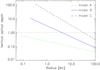 |
Fig. 4 Optical depth perpendicular to the disk as a function of radius at λ = 1.3 mm. |
Above, we have outlined the solution we found in the frame of the settled disk model. However, there may be alternative interpretations of the observed DoAr 33 disk properties that do not call for two distinct grain size distributions. Dullemond & Dominik (2004a) have introduced a self-shadowed disk model to successfully explain the observed SEDs of a group of HAe/Be stars whose SED falls off strongly towards the far-IR, i.e., group II source in Meeus et al. (2001). Self-shadowing is probably induced by the puffed-up inner rim accompanying with grain growth or dust settling in circumstellar disks (Dullemond & Dominik 2004b). The models with a self-shadowed geometry exhibit less mid- to far-IR flux than with a flaring scenario since the outer regions of the disk are indirectly heated by the radiation from the outer parts of the inner rim. A self-shadowed disk therefore can be another explanation for the observations of DoAr 33. However, DoAr 33 is a T Tauri star in which the effect of the inner disk structure such as a puffed-up inner rim on the SED is less pronounced than in the cases of HAe/Be stars, especially when the disk accretion rate is very low (e.g., for DoAr 33 Ṁacc = 2.52 × 10⁻¹⁰ M⊙/yr). Since the inner disk is very close to the central star (Rin = 1 ~ 5 Rsub), a prominent inner rim, if present, would produce much more near-IR (and even some IRAC bands) excess than observed (see Fig. 3). Moreover, the reason self-shadowed geometry appears to our target is complicated. Because the shallow spectral index at (sub)millimeter wavelengths suggests dust growth (Ricci et al. 2010) and dust settling always occurs in circumstellar disks, it is naturally suggested that both grain growth and settling (even with the including an inner rim) should be considered as the cause of self-shadowing for DoAr 33. This is much more difficult to model in detail than our simple two-layer disk solution. Considering the limited observation, we leave this direction open and expect future observations to address the issue.
The SED is a spatially integrated observable that can only provide weak constraints on disk structure because most parameters are degenerated. However, our detailed modeling of DoAr 33 shows that including dust growth and settling in the modeling efforts improves the interpretation of existing data. Follow-up observations are needed to clarify the evolutionary stage of this interesting object, namely dust growth and settling in our context. Herschel far-IR photometry would fill the gap between the mid-IR and (sub)millimeter regimes, hence allows us to better constrain the scale height h100, flaring exponent β, and especially the depletion parameter ϵ of the disk. Our experience with modeling individual protoplanetary disk always leads to the conclusion that spatially resolved images taken at different wavelengths are crucial to constrain the disk parameters (e.g., Wolf et al. 2008; Sauter et al. 2009). Spatially resolved observations at (sub)millimeter wavelengths, e.g., by the Atacama Large Millimeter Array (ALMA) would help break the SED model degeneracies and place additional constraints on the grain size and dust density distribution of the circumstellar disk.
4. Summary
We have conducted a detailed SED modeling study for DoAr 33, a T Tauri star located in the Ophiuchus molecular cloud. Simulated annealing, a versatile optimization technique, was used to search for best-fit parameter sets. We found that a well-mixed disk model fails to explain the observed SED. More specifically, the predicted flux at ~70 μm exceeds the observation. This discrepancy can be explained by dust coagulation and settling because these processes are expected to modify the SED in this way (Andrews et al. 2010). For this reason, we also employed a flared disk with two layers differing in grain size distribution. We fixed the properties of the upper layer to the well-known MRN distribution for ISM dust and left the maximum grain size in the settled grain population as a free parameter to account for dust evolution. Our results show that the predictions obtained with the settled disk model satisfactorily explain the observations in all wavelength regimes. Moreover, the best-fit models we found are less flared than typical T Tauri disks and the best-fit depletion parameter ϵ ~ 0.005 indicates that a considerable portion of small grains has moved towards the disk midplane through coagulation and settling. This is consistent with theories of circumstellar disk evolution. Therefore, DoAr 33 is expected to be a promising target for studying dust growth and settling in protoplanetary disks. We also discussed a self-shadowed disk model as another possible interpretation of the DoAr 33 data. Follow-up observations, especially spatially resolved images, are crucial for breaking the SED model degeneracy and clarifying the evolutionary stage of the circumstellar disk around this interesting object.
Acknowledgments
Y.L. acknowledges support by the German Academic Exchange Service. H.W. acknowledges the support by NSFC grants 10733030, 10921063, and 11173060. This publication makes use of data products from the Wide-field Infrared Survey Explorer, which is a joint project of the University of California, Los Angeles, and the Jet Propulsion Laboratory/California Institute of Technology, funded by the National Aeronautics and Space Administration.
References
- Alexander, R. D., Clarke, C. J., & Pringle, J. E. 2006, MNRAS, 369, 229 [NASA ADS] [CrossRef] [Google Scholar]
- Andrews, S. M., Hughes, A. M., Wilner, D. J., & Qi, C. 2008, ApJ, 678, L133 [NASA ADS] [CrossRef] [Google Scholar]
- Andrews, S. M., Wilner, D. J., Hughes, A. M., Qi, C., & Dullemond, C. P. 2009, ApJ, 700, 1502 [NASA ADS] [CrossRef] [Google Scholar]
- Andrews, S. M., Wilner, D. J., Hughes, A. M., Qi, C., & Dullemond, C. P. 2010, ApJ, 723, 1241 [NASA ADS] [CrossRef] [Google Scholar]
- Balog, Z., Rieke, G. H., Muzerolle, J., et al. 2008, ApJ, 688, 408 [NASA ADS] [CrossRef] [Google Scholar]
- Beckwith, S. V. W., & Sargent, A. I. 1991, ApJ, 381, 250 [NASA ADS] [CrossRef] [Google Scholar]
- Bouvier, J., & Appenzeller, I. 1992, A&AS, 92, 481 [Google Scholar]
- Bouwman, J., Henning, T., Hillenbrand, L. A., et al. 2008, ApJ, 683, 479 [NASA ADS] [CrossRef] [Google Scholar]
- Calvet, N., & Gullbring, E. 1998, ApJ, 509, 802 [NASA ADS] [CrossRef] [Google Scholar]
- Carballido, A., Fromang, S., & Papaloizou, J. 2006, MNRAS, 373, 1633 [NASA ADS] [CrossRef] [Google Scholar]
- Cardelli, J. A., Clayton, G. C., & Mathis, J. S. 1989, ApJ, 345, 245 [NASA ADS] [CrossRef] [Google Scholar]
- Chiang, E. I., & Goldreich, P. 1997, ApJ, 490, 368 [NASA ADS] [CrossRef] [Google Scholar]
- Chiang, E. I., Joung, M. K., Creech-Eakman, M. J., et al. 2001, ApJ, 547, 1077 [NASA ADS] [CrossRef] [Google Scholar]
- Cieza, L. A., Schreiber, M. R., Romero, G. A., et al. 2010, ApJ, 712, 925 [NASA ADS] [CrossRef] [Google Scholar]
- D’Alessio, P., Canto, J., Calvet, N., & Lizano, S. 1998, ApJ, 500, 411 [NASA ADS] [CrossRef] [Google Scholar]
- D’Alessio, P., Calvet, N., & Hartmann, L. 2001, ApJ, 553, 321 [NASA ADS] [CrossRef] [Google Scholar]
- D’Alessio, P., Calvet, N., Hartmann, L., Franco-Hernández, R., & Servín, H. 2006, ApJ, 638, 314 [NASA ADS] [CrossRef] [Google Scholar]
- Dominik, C., Blum, J., Cuzzi, J. N., & Wurm, G. 2007, Protostars and Planets V, 783 [Google Scholar]
- Dullemond, C. P., & Dominik, C. 2004a, A&A, 417, 159 [NASA ADS] [CrossRef] [EDP Sciences] [Google Scholar]
- Dullemond, C. P., & Dominik, C. 2004b, A&A, 421, 1075 [NASA ADS] [CrossRef] [EDP Sciences] [Google Scholar]
- Evans, II, N. J., Dunham, M. M., Jørgensen, J. K., et al. 2009, ApJS, 181, 321 [NASA ADS] [CrossRef] [Google Scholar]
- Furlan, E., Calvet, N., D’Alessio, P., et al. 2005, ApJ, 628, L65 [NASA ADS] [CrossRef] [Google Scholar]
- Furlan, E., Hartmann, L., Calvet, N., et al. 2006, ApJS, 165, 568 [NASA ADS] [CrossRef] [MathSciNet] [Google Scholar]
- Gullbring, E., Hartmann, L., Briceno, C., & Calvet, N. 1998, ApJ, 492, 323 [NASA ADS] [CrossRef] [Google Scholar]
- Hartmann, L., Calvet, N., Gullbring, E., & D’Alessio, P. 1998, ApJ, 495, 385 [NASA ADS] [CrossRef] [Google Scholar]
- Hastings, W. H. 1970, Biometrika, 57, 97 [Google Scholar]
- Hauschildt, P. H., Allard, F., Ferguson, J., Baron, E., & Alexander, D. R. 1999, ApJ, 525, 871 [NASA ADS] [CrossRef] [Google Scholar]
- Juhász, A., Bouwman, J., Henning, T., et al. 2010, ApJ, 721, 431 [NASA ADS] [CrossRef] [Google Scholar]
- Kenyon, S. J., & Hartmann, L. 1995, ApJS, 101, 117 [NASA ADS] [CrossRef] [Google Scholar]
- Kessler-Silacci, J., Augereau, J.-C., Dullemond, C. P., et al. 2006, ApJ, 639, 275 [NASA ADS] [CrossRef] [Google Scholar]
- Kirkpatrick, S., Gelatt, C. D., & Vecchi, M. P. 1983, Science, 220, 671 [NASA ADS] [CrossRef] [MathSciNet] [PubMed] [Google Scholar]
- Lada, C. J. 1999, in The Origin of Stars and Planetary Systems, eds. C. J. Lada, & N. D. Kylafis, NATO ASIC Proc., 540, 143 [Google Scholar]
- Lissauer, J. J., & Stevenson, D. J. 2007, Protostars and Planets V, 591 [Google Scholar]
- Loinard, L., Torres, R. M., Mioduszewski, A. J., & Rodríguez, L. F. 2008, ApJ, 675, L29 [NASA ADS] [CrossRef] [Google Scholar]
- Machida, M. N., Kokubo, E., Inutsuka, S.-I., & Matsumoto, T. 2010, MNRAS, 405, 1227 [NASA ADS] [Google Scholar]
- Meeus, G., Waters, L. B. F. M., Bouwman, J., et al. 2001, A&A, 365, 476 [NASA ADS] [CrossRef] [EDP Sciences] [Google Scholar]
- Metropolis, N., Rosenbluth, A. W., Rosenbluth, M. N., Teller, A. H., & Teller, E. 1953, J. Chem. Phys., 21, 1087 [NASA ADS] [CrossRef] [Google Scholar]
- Natta, A., Testi, L., Neri, R., Shepherd, D. S., & Wilner, D. J. 2004, A&A, 416, 179 [NASA ADS] [CrossRef] [EDP Sciences] [Google Scholar]
- Nomura, H., & Nakagawa, Y. 2006, ApJ, 640, 1099 [NASA ADS] [CrossRef] [Google Scholar]
- Nourani, Y., & Andresen, B. 1998, J. Phys. A-Math. Gen., 31, 8373 [NASA ADS] [CrossRef] [Google Scholar]
- Orellana, M., Cieza, L. A., Schreiber, M. R., et al. 2012, A&A, 539, A41 [NASA ADS] [CrossRef] [EDP Sciences] [Google Scholar]
- Papaloizou, J. C. B., & Terquem, C. 2006, Rep. Prog. Phys., 69, 119 [Google Scholar]
- Pinte, C., Padgett, D. L., Ménard, F., et al. 2008, A&A, 489, 633 [NASA ADS] [CrossRef] [EDP Sciences] [Google Scholar]
- Pollack, J. B., Hubickyj, O., Bodenheimer, P., et al. 1996, Icarus, 124, 62 [NASA ADS] [CrossRef] [Google Scholar]
- Ricci, L., Testi, L., Natta, A., & Brooks, K. J. 2010, A&A, 521, A66 [NASA ADS] [CrossRef] [EDP Sciences] [Google Scholar]
- Roberts, G. O., Gelman, A., & Gilks, W. R. 1997, Ann. Appl. Prob., 7, 110 [Google Scholar]
- Robitaille, T. P., Whitney, B. A., Indebetouw, R., Wood, K., & Denzmore, P. 2006, ApJS, 167, 256 [NASA ADS] [CrossRef] [Google Scholar]
- Sauter, J., & Wolf, S. 2011, A&A, 527, A27 [NASA ADS] [CrossRef] [EDP Sciences] [Google Scholar]
- Sauter, J., Wolf, S., Launhardt, R., et al. 2009, A&A, 505, 1167 [NASA ADS] [CrossRef] [EDP Sciences] [Google Scholar]
- Schegerer, A., Wolf, S., Voshchinnikov, N. V., Przygodda, F., & Kessler-Silacci, J. E. 2006, A&A, 456, 535 [NASA ADS] [CrossRef] [EDP Sciences] [Google Scholar]
- Schräpler, R., & Henning, T. 2004, ApJ, 614, 960 [NASA ADS] [CrossRef] [Google Scholar]
- Shakura, N. I., & Sunyaev, R. A. 1973, A&A, 24, 337 [NASA ADS] [Google Scholar]
- Testi, L., Natta, A., Shepherd, D. S., & Wilner, D. J. 2001, ApJ, 554, 1087 [Google Scholar]
- van Boekel, R., Min, M., Waters, L. B. F. M., et al. 2005, A&A, 437, 189 [NASA ADS] [CrossRef] [EDP Sciences] [Google Scholar]
- Walker, C., Wood, K., Lada, C. J., et al. 2004, MNRAS, 351, 607 [NASA ADS] [CrossRef] [Google Scholar]
- Weidenschilling, S. J. 1977, Ap&SS, 51, 153 [Google Scholar]
- Weingartner, J. C., & Draine, B. T. 2001, ApJ, 548, 296 [NASA ADS] [CrossRef] [Google Scholar]
- Wilking, B. A., Meyer, M. R., Robinson, J. G., & Greene, T. P. 2005, AJ, 130, 1733 [NASA ADS] [CrossRef] [Google Scholar]
- Wolf, S. 2003, Comp. Phys. Commun., 150, 99 [Google Scholar]
- Wolf, S., Padgett, D. L., & Stapelfeldt, K. R. 2003, ApJ, 588, 373 [NASA ADS] [CrossRef] [Google Scholar]
- Wolf, S., Schegerer, A., Beuther, H., Padgett, D. L., & Stapelfeldt, K. R. 2008, ApJ, 674, L101 [NASA ADS] [CrossRef] [Google Scholar]
Appendix A: Description of simulated annealing
A common method for fitting model parameters to an observed SED is to precalculate a database for a given disk model and dust properties on a huge grid in parameter space (e.g., Robitaille et al. 2006). The main advantage of this approach is that a single set of observations can be fitted very fast by evaluating the merit function, i.e., the χ2-distribution, once the database is built. However, the number of grid points increases substantially with the dimensionality of the parameter space. The model grid is always a compromise between finite computational resources and resolution. It is therefore impractical to search on a sufficiently fine grid in parameter space since realistic models usually contain too many dimensions.
Simulated annealing (SA) is a versatile optimization technique based on the Metropolis-Hastings algorithm, and it has been used for many optimization challenges (Kirkpatrick et al. 1983). The main idea is to emulate the cooling of a melt by first introducing small and random perturbations (e.g., heating) into the system and then slowly cooling the system in a controlled manner to obtain the “lowest energy state”, i.e. the global optimum. In practice, SA constructs a random walk, i.e. a Markov chain, through the parameter space, thereby minimizing the discrepancy between observation and prediction by following the local topology of the merit function. Local minima can be overcome intrinsically regardless of the dimensionality and points near optima will be evaluated with higher probability. Considering 11 degrees of freedom of our model (see Table A.1), we employed SA to search for optimum solutions to the merit function in our study defined by ![Mathematical equation: \appendix \setcounter{section}{1} \begin{equation} \chi^{2} = \sum_{i=1}^{n}\frac{\left[F_{i}\left({\rm simu}\right)-F_{i}\left(\rm{obs}\right)\right]^2}{\Delta{F_{i}^{2}\left(\rm{obs}\right)}}\cdot \end{equation}](/articles/aa/full_html/2012/10/aa19336-12/aa19336-12-eq87.png) (A.1)Here, n is the number of photometric data points, Fi(simu) the simulated flux, Fi(obs) the observation, and ΔFi(obs) the photometric uncertainty. Notably, two different results for the flux measured by MIPS at 70 μm have been independently published by Evans et al. (2009) and Cieza et al. (2010). The former gave a definite detection of DoAr 33, and the latter proposed an upper limit. We only took the real detection into account for the calculation of total χ2.
(A.1)Here, n is the number of photometric data points, Fi(simu) the simulated flux, Fi(obs) the observation, and ΔFi(obs) the photometric uncertainty. Notably, two different results for the flux measured by MIPS at 70 μm have been independently published by Evans et al. (2009) and Cieza et al. (2010). The former gave a definite detection of DoAr 33, and the latter proposed an upper limit. We only took the real detection into account for the calculation of total χ2.
Starting points of the Markov chains for both disk scenarios.
Initial step widths and boundary of the parameter space.
Construction of Markov chains: A sequence of parameter sets is created during the optimization process. Since every sequence element is deduced from its predecessor, this sequence constitutes a Markov chain. Starting from an arbitrary point, a random walk through parameter space is generated by sampling the possible increments Δa from a Gaussian distribution ![Mathematical equation: \appendix \setcounter{section}{1} \begin{equation} \rm{Prob}(\Delta{a}) \sim \prod_k\exp\left[-\frac{\Delta a_k^2}{2\beta_k^2}\right], \end{equation}](/articles/aa/full_html/2012/10/aa19336-12/aa19336-12-eq114.png) (A.2)where βk is the step sizes with the index k ∈ {1,...,D} listing all parameter dimensions. Table A.1 lists five different starting models we considered, and the boundary of the parameter space is described in Table A.2. To ensure randomness of our sampling process, three different seeds were used to initialize the pseudo-random number sequence for each of the five starting points, resulting in a total number of 15 different Markov chains.
(A.2)where βk is the step sizes with the index k ∈ {1,...,D} listing all parameter dimensions. Table A.1 lists five different starting models we considered, and the boundary of the parameter space is described in Table A.2. To ensure randomness of our sampling process, three different seeds were used to initialize the pseudo-random number sequence for each of the five starting points, resulting in a total number of 15 different Markov chains.
Accept/reject the new step: After calculating the chi-square  of a new proposed model, the choice of accepting/rejecting should be made to determine the current position in parameter space. There are two possibilities according to the Metropolis-Hastings algorithm (Metropolis et al. 1953; Hastings 1970). First, the new model is directly accepted when the
  is less than the chi-square of the last accepted step
  . To make the choice only in this way always leads to a solution with local, but not necessarily a general, χ2 minimum. Second, if
  , we evaluate the so-called Boltzman probability distribution:
 ![Mathematical equation: \appendix \setcounter{section}{1} \begin{equation} {\rm Prob}=\rm{exp}\left[-\frac{\chi^{2}_{\rm{new}}-\chi^{2}_{\rm{last}}}{\tau}\right]\cdot \end{equation}](/articles/aa/full_html/2012/10/aa19336-12/aa19336-12-eq122.png) (A.3)In the meantime, a uniformly distributed random number u within the range [0,1] is generated, and the new step will be taken only if u < Prob. In doing so, there is a corresponding chance for the system to get out of a local minimum in favor of finding a better, more general one.
(A.3)In the meantime, a uniformly distributed random number u within the range [0,1] is generated, and the new step will be taken only if u < Prob. In doing so, there is a corresponding chance for the system to get out of a local minimum in favor of finding a better, more general one.
Cooling scheme: The system temperature τ is a major parameter to control movements of the random walk in parameter space and should be gradually decreased to steer the Markov chain to the vicinity of the global optimum. Various cooling schemes have been proposed and compared with the goal of achieving a fast convergence (Nourani & Andresen 1998). Technically speaking, the choice of cooling scheme highly depends on the optimization problem at hand. As a complex cooling scheme always contains several free parameters that must be adjusted empirically, we adopt a non-monotonic and self-regulating strategy by setting the system temperature τ after every accepted step to  (A.4)Nevertheless, γ has to be adjusted empirically and we use γ = 0.25. As is suggested by Roberts et al. (1997), the total acceptance ratio
  should be in the vicinity of 0.234. To meet this demand, we monitored previous steps and adjusted the step widths βk by analyzing the relative step widths in accepted and rejected steps of the chain. Additionally, the temperature will be increased for every step with
  if the total acceptance ratio drops below 0.10 to avoid getting trapped at a deep local optimum.
Adaptive step sizes: The step size βk is a main parameter that controls the displacement between the two adjacent positions in the Markov chain. Optimal step sizes cannot be defined at the beginning since no information is available on the distribution under investigation. The step sizes for each of the parameters have to be adapted along the optimization run. For this purpose, the reasonable initial values that are dependent on the starting points of the Markov chain are listed in Table A.2.
We define a local acceptance ratio of the chain using the sequence ηn ∈ {0,1} of rejected and accepted steps by calculating  (A.5)for some constant lookback length l < n, where n refers to the step count. To maintain the optimal acceptance ratio in the vicinity of ξ0 = 0.234, we implement a control loop that adjusts the step widths βk by analyzing the last l = 25 positions of the chain. The algorithm calculates the moduli of relative changes between the proposed parameter an,k and the previously accepted parameter
  :
:  (A.6)By separately summing up the relative changes cn,k for every parameter in accepted and rejected proposals, two vectors gn,k and bn,k can be derived to describe the impact of good and bad decisions,
  (A.7)if ξn > ξ0, the step size of the parameter with the smallest components in gn,k is increased to encourage riskier proposals. On the contrary, if ξn < ξ0 the step size of the parameter with the largest component in bn,k is decreased to induce more conservative proposals. In either case the step size of the selected parameter is adjusted by multiplying with the factor of (1 − ξ0) + ξn.
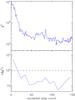 |
Fig. A.1 The evolution of χ2 and ⟨ Δχ2 ⟩ for Markov chain IV running with the settled disk model. The diamond in the upper panel marks the minimum χ2 position. |
Additionally, the step sizes are controlled to be <50% and >1% of the current parameter values in order to avoid large fluctuations and extremely slow convergence of the Markov chain respectively.
Chain abortion: Since no upper bound for the step count to reach the global optimum can be given, we must define a reasonable criterion to stop an optimization run. Because the system temperature τ is coupled to the χ2 of the currently accepted model (see Eq. (A.4)), the probability of escaping a local minimum does not converge asymptotically towards zero (see Eq. (A.3)). It is thus not straightforward to decide when to abort the Markov chain using a system temperature threshold as normally implemented (e.g., Nourani & Andresen 1998). Instead, we analyze the quality of the fit for every accepted model of an individual Markov chain. The variation in the fitting quality is evaluated by calculating the difference Δχ2 between two adjacent accepted steps. A particular Markov chain is aborted if the box average ⟨ Δχ2 ⟩ remained below a threshold for a certain number of steps Nabort in a row. We used  and Nabort ~ 100 steps and averaged with a box of ten samples. An illustration of this idea is shown in Fig. A.1, for example of Chain IV. The best fit was defined as that with the lowest χ2 found among all iterations. Here, we emphasize that our criteria of chain abortion is not universal since the solution highly depends on the problem at hand because the χ2-distributions are not identical between different optimization problems.
All Tables
All Figures
|
Fig. 1 SED data of DoAr 33: WIYN (Wilking et al. 2005), 2MASS, IRAC, and MIPS (Evans et al. 2009), WISE (WISE All Sky Data Release 2012), MIPS upper limit at 70 μm (red triangle, Cieza et al. 2010), SCUBA and IRAM (Andrews et al. 2007), ATCA (Ricci et al. 2010). |
| In the text | |
|
Fig. 2 Dust density distribution normalized to the maximum on a plane perpendicular to the disk midplane. For better graphical representation, the fourth root of the function is plotted. Upper plot: disk model with the inclusion of dust settling. Large grains dominate the density in the midplane, while small grains are present everywhere in the disk. Lower plot: well-mixed model in which the grain size distribution is homogeneous at all disk radii. |
| In the text | |
|
Fig. 3 The top three model fits found by SA. The red diamonds depict the photometric measurements and the black arrow represents the upper limit for the 70 μm flux (Cieza et al. 2010). The gray dotted line marks the contribution of the central star to the total flux of the system. |
| In the text | |
|
Fig. 4 Optical depth perpendicular to the disk as a function of radius at λ = 1.3 mm. |
| In the text | |
|
Fig. A.1 The evolution of χ2 and ⟨ Δχ2 ⟩ for Markov chain IV running with the settled disk model. The diamond in the upper panel marks the minimum χ2 position. |
| In the text | |
Current usage metrics show cumulative count of Article Views (full-text article views including HTML views, PDF and ePub downloads, according to the available data) and Abstracts Views on Vision4Press platform.
Data correspond to usage on the plateform after 2015. The current usage metrics is available 48-96 hours after online publication and is updated daily on week days.
Initial download of the metrics may take a while.