| Issue |
A&A
Volume 546, October 2012
|
|
|---|---|---|
| Article Number | A15 | |
| Number of page(s) | 14 | |
| Section | Extragalactic astronomy | |
| DOI | https://doi.org/10.1051/0004-6361/201219285 | |
| Published online | 28 September 2012 | |
Globular cluster systems in fossil groups: NGC 6482, NGC 1132, and ESO 306-017⋆
1 European Southern Observatory, Alonso de Córdova 3107, Vitacura, Santiago, Chile
2 Centro de Radioastronomía y Astrofísica, Universidad Nacional Autónoma de México, 58090 Morelia, México
e-mail: This email address is being protected from spambots. You need JavaScript enabled to view it.
3 Dominion Astrophysical Observatory, Herzberg Institute of Astrophysics, National Research Council of Canada, Victoria, BC V9E 2E7, Canada
4 Departamento de Astronomía y Astrofísica, Pontificia Universidad Católica de Chile, 7820436 Macul, Santiago, Chile
5 Department of Physics, University of California, Davis, CA 956160, USA
6 Institute for Geophysics and Planetary Physics, Lawrence Livermore National Laboratory, L-413, Livermore, CA 94550, USA
7 School of Mathematics and Physics, The University of Queensland, Brisbane, QLD 4072, Australia
8 Argelander-Institut für Astronomie, Auf dem Hügel 71, 53121 Bonn, Germany
Received: 26 March 2012
Accepted: 14 August 2012
Abstract
We study the globular cluster (GC) systems in three representative fossil group galaxies: the nearest (NGC 6482), the prototype (NGC 1132) and the most massive known to date (ESO 306-017). This is the first systematic study of GC systems in fossil groups. Using data obtained with the Hubble Space Telescope Advanced Camera for Surveys in the F475W and F850LP filters, we determine the GC color and magnitude distributions, surface number density profiles, and specific frequencies. In all three systems, the GC color distribution is bimodal, the GCs are spatially more extended than the starlight, and the red population is more concentrated than the blue. The specific frequencies seem to scale with the optical luminosities of the central galaxy and span a range similar to that of the normal bright elliptical galaxies in rich environments. We also analyze the galaxy surface brightness distributions to look for deviations from the best-fit Sérsic profiles; we find evidence of recent dynamical interaction in all three fossil group galaxies. Using X-ray data from the literature, we find that luminosity and metallicity appear to correlate with the number of GCs and their mean color, respectively. Interestingly, although NGC 6482 has the lowest mass and luminosity in our sample, its GC system has the reddest mean color, and the surrounding X-ray gas has the highest metallicity.
Key words: galaxies: elliptical and lenticular, cD / galaxies: star clusters: general / galaxies: groups: general / galaxies: individual: NGC 6482 / galaxies: individual: NGC 1132 / galaxies: individual: ESO 306-017
Based on observations made with the NASA/ESA Hubble Space Telescope, obtained at the Space Telescope Science Institute, which is operated by the Association of Universities for Research in Astronomy, Inc., under NASA contract NAS 5-26555. These observations are associated with program # 10558.
© ESO, 2012
1. Introduction
The most accepted mechanism of galaxy formation is hierarchical assembly, whereby large structures are formed by the merging of smaller systems (Press & Schechter 1974; De Lucia et al. 2006); nevertheless, there are some open questions and this scenario is debated (Nair et al. 2011; see also Sales et al. 2012). The hierarchical assembly is supported by the frequent observation of galactic interactions, and predicts that all the galaxies within a galaxy group or cluster will eventually merge into a single massive elliptical galaxy; this would be the last step of galaxy formation. Indeed, Ponman et al. (1994) found an extreme system consisting of a giant elliptical galaxy surrounded by dwarf companions, all immersed in an extended X-ray halo. This system was interpreted as the end product of the merger of galaxies within a group, and was thus called a fossil group (FG). A formal definition was introduced by Jones et al. (2003), according to which FGs are systems with  , and an optical counterpart where the difference in magnitude between the first and the second brightest galaxies is ΔmR > 2 mag. Because of their regular X-ray morphologies and lack of obvious recent merger activity, FG galaxies are usually considered to be ancient and unperturbed systems (Khosroshahi et al. 2007). This is supported by numerical simulations that suggest FGs formed at early epochs (z > 1) and afterwards evolved fairly quiescently (D’Onghia et al. 2005; Dariush et al. 2007; Díaz-Giménez et al. 2011).
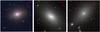 |
Fig. 1 ACS color images, FOV |

At present, there is no consensus on the mass-to-light ratios (M/L) of FGs; measurements span from ~100 M⊙/L⊙ (Khosroshahi et al. 2004) to ~1000 M⊙/L⊙ (Vikhlinin et al. 1999; Yoshioka et al. 2004; Cypriano et al. 2006) in the R-band, but there is a tendency toward higher values (Proctor et al. 2011; Eigenthaler & Zeilinger 2012). Such high M/L values, together with the fact that FGs show unusually high LX/Lopt ratios compared with typical galaxy groups, appear inconsistent with the assumption that FGs are formed by the merging of the members in ordinary galaxy groups (see Fig. 2 in Khosroshahi et al. 2007). Compact galaxy groups in the nearby universe tend to have lower masses and X-ray luminosities than observed in FGs, although there is evidence that high-mass compact groups may have been more common in the past and could represent the progenitors of today’s FGs (Mendes de Oliveira & Carrasco 2007). In addition, the optical luminosities of the dominant giant ellipticals in FGs (Khosroshahi et al. 2006; Tovmassian 2010) are similar to those of brightest cluster galaxies (BCGs). For these reasons, it has been suggested that FGs are more similar to galaxy clusters, but simply lack other early-type galaxies with luminosities comparable to the central galaxy (Mendes de Oliveira et al. 2009). It remains an open question whether FGs represent the final phase of most galaxy groups, or if they constitute a distinct class of objects which formed with an anomalous top-heavy luminosity function (Cypriano et al. 2006; Cui et al. 2011; see also Méndez-Abreu et al. 2012).
Globular clusters (GC) systems are a powerful tool to study galaxy assembly (Fall & Rees 1985; Harris 1991; Forbes et al. 1997; West et al. 2004; Brodie & Strader 2006). GCs are among the oldest objects in the universe, and dense enough to survive galactic interactions. Most of them have ages older than 10 Gyr (Cohen et al. 1998; Puzia et al. 2005), and therefore probably formed before or during galaxy assembly. The correlation of the optical luminosity of a galaxy with the mean metallicities of the field stars and GCs (van den Bergh 1975; Brodie & Huchra 1991; Forbes et al. 1996; Côté et al. 1998) supports the idea that GC and galaxy formation are strongly linked. Nevertheless, there is a shift in metallicity, in the sense that field stars are on average more metal-rich than GCs. Interestingly, Cohen et al. (1998) noted that the metallicity of the X-ray gas in M 87 is similar to the metallicity of the field stars. Thus, the GC population could constitute a record of the initial chemical enrichment of the parent galaxy.
Sample data.
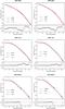 |
Fig. 2 Galaxy surface brightness distribution as a function of the isophotal equivalent circular radius Rc. The dots are the data after subtraction of the fitted sky value. The solid red lines show the best fit profiles: single Sérsic for NGC 6482 and core-Sérsic for NGC 1132 and ESO 306-017. For the galaxies where the best fit is core-Sérsic, the dashed blue line shows the single Sérsic. Top to bottom: NGC 6482, NGC 1132 and ESO 306-017. The left and right panels are the g and z band, respectively. For ESO 306-017, the gray dots were not included in the fit. |
The GC systems of massive early-type galaxies are generally bimodal in their optical color distributions (Zepf & Ashman 1993; Geisler et al. 1996; Gebhardt & Kissler-Patig 1999). The two GC color components are commonly referred to as the metal-poor (blue) and metal-rich (red) subpopulations, and could indicate distinct major episodes of star formation. In the Milky Way, spectroscopic studies reveal two populations of GCs with distinct metallicities (Zinn 1985). However, the situation is less clear for giant ellipticals and other massive galaxies with more complex formation histories, which may simply have broad metallicity distributions with a nonlinear dependence of color on metallicity (Yoon et al. 2006, 2011; Blakeslee et al. 2012; Chies-Santos et al. 2012). Another important property of GC systems is their luminosity function (GCLF). The GCLF is well described by a Gaussian with peak at  , and the dispersion for giant ellipticals with well-populated GC systems is
  (Harris 1991). The general homogeneity of the GCLF is unexpected a priori, given that GC destruction mechanisms should depend on the environment (McLaughlin & Fall 2008). However, recent studies show that the GCLF dispersion depends on galaxy luminosity (Jordán et al. 2007b; Villegas et al. 2010).
The most basic measure of a GC system is its richness, or the total number of GCs in the system. Harris & van den Bergh (1981) introduced the concept of specific frequency, SN, as the number of GCs per unit galaxy luminosity, normalized to a galaxy with absolute V magnitude MV = −15. They reported values in the range 2 < SN < 10 for elliptical galaxies. However, they also already noted that M 87, the central galaxy in the Virgo cluster, had an outstandingly large value of SN ~ 20 (a more recent value from Peng et al. 2008, is SN = 12.6 ± 0.8); hence, they suggested that environment may play a role in GC formation. Later, other high-SN galaxies were identified, most of them being either BCGs or second brightest galaxies in clusters; often, these galaxies were classified as type cD, however not all galaxies classified as cD have high SN (Jordán et al. 2004). It is interesting to note that, although BCGs have quite a uniform luminosity, to the point of being considered standard candles (Postman & Lauer 1995), they have a wide range in SN. Conversely, Blakeslee et al. (1997) found a correlation between SN of the BCG and the velocity dispersion and X-ray luminosity of the cluster. They therefore suggested that the number of GCs scales roughly with cluster mass, a fact that suggests that galaxies with high values of SN, like M 87, are not anomalously rich in GCs but, rather, underluminous as a consequence of the lower overall star formation efficiency in more massive and denser systems (Blakeslee 1999; Peng et al. 2008).
Hence, given that FGs appear to be ancient, highly luminous, but relatively unperturbed systems with origins that remain poorly understood (identified less than two decades ago), we study for the first time the GC populations of the dominant elliptical. We also compare our measured GC properties with X-ray properties obtained from the literature, and look for photometric irregularities that could be signs of recent galactic interactions. To have a representative sample we choose: the nearest, NGC 6482 (z = 0.013), the prototype, NGC 1132 (z = 0.023), and the most massive known to date, ESO 306-017 (z = 0.036), shown in Fig. 1. In the following section, we describe the observations, data processing, and GC selection criteria; in Sect. 3, we analyze the photometry and present our measurements; in Sect. 4, we discuss the implications of our results in the larger context of FG and early-type galaxy formation scenarios. The final section summarizes our conclusions. Throughout, we estimate distances assuming H0 = 71 km s-1 Mpc-1.
2. Observations and reductions
The observations were taken with the Advanced Camera for Surveys on board the Hubble Space Telescope (HST), using the Wide Field Channel with the F475W ( ≈ the g passband of the Sloan Digital Sky Survey, SDSS) and F850LP (≈SDSS z) filters (GO proposal 10558).
The broadband g and z filters offer relatively high throughput and g − z color is very sensitive to age and metallicity variations (Côté et al. 2004). The integration time for each galaxy was chosen to reach the expected turnover magnitude of the GCLF,  and
and  (Jordán et al. 2007b), assuming a Gaussian distribution. Table 1 lists the redshift, distance modulus, exposure time and expected apparent turnover magnitude of the GCLF for each filter, as well as the physical scale corresponding to 1 arcsec. The ACS pixel scale is 0.05 arcsec pixel-1.
For all images the same data reduction procedure was followed. Geometrical correction, image combination, and cosmic ray rejection were done with the data reduction pipeline APSIS (Blakeslee et al. 2003). A point spread function (PSF) model was constructed for each image using the DAOPHOT (Stetson 1987) package within IRAF (Tody 1986). The best fitting function for all the images was Moffat25 (good for undersampled data), with FWHM ~ 2 pixels and fitting radius = 3 pixels.
2.1. Galaxy surface brightness distribution
We are interested in the detection and magnitudes of GCs, which can be affected by drastic changes in the background due to the galaxy light (mainly in the inner region). Hence, to perform the detections over an image with nearly flat background it is necessary to subtract the galaxy light.
To model the galaxy light, the brightest objects (foreground stars, background and group galaxies) were masked, and subsequently the surface brightness distribution of the central giant elliptical was modeled with the ellipse (Jedrzejewski 1987) and bmodel tasks within the STSDAS1 package in IRAF. A second mask was made for objects detected at > 4.5σ with SExtractor (Bertin & Arnouts 1996) in the galaxy-subtracted image. A second, final model of the surface brightness distribution of the stellar component (galaxy model) was produced from the newly masked image.
Due to the relatively small ACS field-of-view (FOV;  ), the giant ellipticals fill the images, and it is not possible to measure an absolute sky value directly. Thus, a surface brightness radial profile of galaxy plus sky was constructed.
Although the value of the sky is not a critical issue for calculating colors of GCs, since a local value of the sky is measured for each of them, a reliable estimate of the sky level is essential to measure the magnitude of the galaxy, which is needed to obtain SN. Thus, to estimate a realistic sky value, we assumed that the starlight follows a Sérsic profile (Sérsic 1968), which provides a good description of the outer parts of early-type galaxies (Trujillo et al. 2004; Ferrarese et al. 2006). We fit, to the constructed intensity radial profile, the function: ![Mathematical equation: \begin{equation} I(r)=I_{\rm e}\exp\left\{-b_n \left[ {\left( \frac{r}{R_{\rm e}}\right) }^{1/n}- 1\right] \right\} + I_{\rm sky} \end{equation}](/articles/aa/full_html/2012/10/aa19285-12/aa19285-12-eq44.png) (1)where Re is the effective radius that encloses half of the light; Ie is the effective intensity at Re; n is the Sérsic index, which indicates the slope; Isky is the sky intensity; bn ≈ 1.9992n − 0.3271 (Graham & Driver 2005). The technique to estimate the best fit model was χ2 minimization, using the task Optim inside R: a Language and Environment for Statistical Computing2. Optim uses the algorithm of Nelder-Mead (1965), which is based on the concept of a simplex, searching for the minimum by comparing the function values on vertices in parameter space. We tried various starting parameters to avoid local minima.
(1)where Re is the effective radius that encloses half of the light; Ie is the effective intensity at Re; n is the Sérsic index, which indicates the slope; Isky is the sky intensity; bn ≈ 1.9992n − 0.3271 (Graham & Driver 2005). The technique to estimate the best fit model was χ2 minimization, using the task Optim inside R: a Language and Environment for Statistical Computing2. Optim uses the algorithm of Nelder-Mead (1965), which is based on the concept of a simplex, searching for the minimum by comparing the function values on vertices in parameter space. We tried various starting parameters to avoid local minima.
The fits were done independently for each filter. Each point was weighted by a factor ϵI, where I is the point’s intensity and ϵ is chosen to obtain χ2 ~ 1 (Byun et al. 1996; Ferrarese et al. 2006); we used ϵ = 0.05, 0.01 and 0.03 for NGC 6482, NGC 1132, and ESO 306-017, respectively. We performed two fits, one with all the parameters free, and a second fixing n = 4. For NGC 1132 and ESO 306-017, the sky values obtained for the n = 4 fits were higher than the mean background values in lowest regions of the images, which suggests that the sky levels obtained with these fits were overestimated. Moreover, with n as a free parameter, we recovered higher values (n > 4) in line with expectations for such luminous galaxies; thus, we favor the fits with n free (Graham et al. 1996; La Barbera et al. 2012).
We next subtracted the estimated sky value and converted the semi-major axis of each isophote to the equivalent circular radius (or geometric radius), Rc, following the relation:  , where q here is the axis ratio of the isophote. We then performed a second fit to the sky-subtracted, circularized μSB profile (Fig. 2). This approach allows for direct comparisons with literature values (e.g., Ferrarese et al. 2006).
As seen from the fitted profiles, there is less light in the inner regions of NGC 1132 and ESO 306-017 than predicted by the Sérsic profile (blue dashed lines). This is a common feature in giant ellipticals. Studies of the surface brightness, μSB, profiles of early-type galaxies spanning a range in luminosity have revealed that the most luminous ellipticals often show central deficits, or “cores”, with respect to the inward extrapolation of the best-fit Sérsic models, whereas intermediate-luminosity early-type galaxies are generally well described by Sérsic models at all radii (Ferrarese et al. 2006; Côté et al. 2007). At fainter luminosities, early-type dwarf galaxies tend to possess central excesses, or “nuclei”.
Hence, we add a core component (Trujillo et al. 2004; Graham & Driver 2005; Ferrarese et al. 2006) to the function to improve the models for these high-luminosity galaxies. The core-Sérsic function is: ![Mathematical equation: \begin{eqnarray} I(r)&=&I_{\rm b} 2^{-(\gamma/\alpha)} \exp \left[ b\left(2^{1/\alpha}\frac{R_{\rm b}}{R_{\rm e}}\right)^{1/n} \right] \nonumber\\ &&\quad\times {\left[ 1+\left(\frac{R_{\rm b}}{r}\right)^{\alpha} \right]}^{\gamma/\alpha} \times \exp\left\{ -b \left[ \frac{R^{\alpha} +{R_{\rm b}}^{\alpha} }{{R_{\rm e}}^{\alpha}} \right] ^{1/(\alpha{n})}\right\} + I_{\rm sky} \end{eqnarray}](/articles/aa/full_html/2012/10/aa19285-12/aa19285-12-eq61.png) (2)where Rb is the break radius (transition point between Sérsic and inner power-law), Ib is the intensity at Rb, α indicates how sharp is the transition, and γ is the slope of the inner component.
(2)where Rb is the break radius (transition point between Sérsic and inner power-law), Ib is the intensity at Rb, α indicates how sharp is the transition, and γ is the slope of the inner component.
Best galaxy surface brightness model parameters in g and z bands: single Sérsic for NGC 6484 and core-Sérsic for NGC 1132 and ESO 306-017.
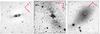 |
Fig. 3 Residual images after subtracting the best single Sérsic model, in z band: NGC 6482 (left), NGC 1132 (center), and ESO 306-017 (right). The galaxies are shown at the observed orientation. |
For ESO 306-017 we can see a feature around log 10(r) ~ 1.7, that might be stripped material from the second brightest galaxy in the image, resulting in an excess of light. Consequently, we reject the range 12.5′′ < r < 90′′ from the fit domain in both filters (gray dots in Fig. 2), whereupon we obtain a good fit. Nonetheless, Sun et al. (2004) reported a steeper profile over a larger spatial range using ground-based data in the R-band, with the profile declining more sharply than n = 4 at large radii. It would be unusual for a galaxy with such high luminosity to have n < 4. The inconsistency in n values at different radii in this galaxy reflects the peculiarity of its light profile, indicating that a single Sérsic model does not provide an adequate description. We therefore encourage the reader to be cautious in interpreting or using the fitted surface brightness parameters for this galaxy. For the more regular galaxy NGC 1132, Schombert & Smith (2012) reported n = 7.1 and a circular effective radius  , both of which are close to our fitted values. Table 2 lists our final best-fit Sérsic parameters and sky values.
Elliptical galaxies are well described by Sérsic profiles unless they are disturbed due to recent interaction (Ferrarese et al. 2006). To detect any signature of disturbances, we constructed galaxy models based on the Sérsic parameters obtained from fitting the bmodel profile. The best single Sérsic parameters were used to construct model images using the program BUDDA (de Souza et al. 2004). Because the fit we obtained is in one dimension, to construct the 2D model we needed to assign an ellipticity and positional angle (PA), which are taken from the ellipse fit. These values are nearly constant except in the very inner region (see Fig. 9), probably due to dust or inner structures. Thus, we chose the mean values of ellipticity and PA of the outer region isophotes (r > 30 arcsec). Afterwards, these models were subtracted from the original images. For NGC 1132 we see residuals with an appearance of shells; to rule out that these are caused by a bad choice of PA value, we constructed model images changing the PA; we recovered the shell-like structure in all cases.
The existence of dust lanes is evident in the inner regions of all three FGs (Fig. 4). Furthermore, the residual images (Fig. 3) show evidence of galactic interaction: apparent shells in NGC 1132, a tidal tail in ESO 306-017 and an inner disk in NGC 6482. It must be noted that these features contradict the claims of previous authors, who did not find signs of merger activity (Jones et al. 2003; Khosroshahi et al. 2004). This point shall be discussed in Sect. 5.
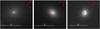 |
Fig. 4 Inner regions of g-band images: NGC 6482 (left), NGC 1132 (center), and ESO 306-017 (right). Dust is present in all cases. |
2.2. Globular cluster selection
Based on their recession velocities, NGC 6482, NGC 1132, and ESO 306-017 are located at 56, 99, and 155 Mpc, respectively (Table 1); GCs which have typical half-light radii of ~3 pc (Jordán et al. 2005), will be unresolved and appear as an excess of point sources over the foreground stars and small background galaxies. The number of these contaminants can be estimated using control fields.
The detection and photometry of GC candidates were done with SExtractor, using rms maps that indicate the weight of each pixel according to read noise, cosmic rays and saturated pixels. The confidence in the detections is naturally greater for brighter objects, but reaching fainter magnitudes allows a better sampling of the GCLF. Aiming at a compromise between GCLF completeness and good rejection of spurious detections, we chose a threshold of 1.5σ per pixel, and a minimum area for a positive detection MINAREA = 5 pixels; together, these constraints imply a minimum effective detection threshold of 3.35σ. An initial sample was constructed with objects detected independently in both g and z filters, with matching coordinates within a radius of 2 pixels, ellipticity lower than 0.3 and CLASS_STAR3 greater than 0.7.
We adopt the photometric AB system, for which the zero points are zpg = 26.081 and zpz = 24.8674. These values are valid for an infinite aperture; we use aperture photometry (with a 3 pixel radius), and apply an appropriate aperture correction (Sirianni et al. 2005). Magnitudes are corrected for foreground extinction using the reddening maps of Schlegel et al. (1998) for each field and filter. The extinction transformations to g and z are Ag = 3.634 E(B − V) and Az = 1.485 E(B − V). E(B − V) values for NGC 6482, NGC 1132, and ESO 306-017 are 0.099, 0.065, 0.0335, respectively.
Objects five magnitudes brighter than the expected turnover magnitude, m0, in both filters (mg,z < m0g,z − 5, see Table 1), were rejected from the GC sample as they are undoubtedly contaminants. With this cut we reject ≲ 0.02% of the brightest GCs, but we avoid foreground stars.
Objects with reddening-corrected color 0.5 < g − z < 2.0 were kept; single stellar populations with age in the range 2−15 Gyr and metallicity −2.25 < [Fe/H] < + 0.56 lie in this range (Côté et al. 2004). Finally, the selected sample of GC candidates was cleaned of objects with an uncertainty in magnitude larger than 0.2 mag in order to have objects with reliable magnitudes.
To determine the GC detection completeness as a function of magnitude, ~25 000 artificial stars were constructed based on the PSF of each image, with magnitudes in the interval 22 < mstar < 29, and color 0.7 < gstar − zstar < 1.7, where most GCs lie. This color range is slightly narrower than the color criteria for GCs because we needed to take into account the dispersion in the magnitude measurements (Fig. 5). Only ~100 stars were added randomly at a time, to avoid crowding and overlapping with original objects. Afterwards, each image was analyzed exactly the same way as the original data. Pritchet curve (Fleming et al. 1995) fitted to the fraction of recovered stars versus magnitude provides our completeness function (Fig. 6). Based on the completeness test we are confident that the detection is ≳ 90% complete at z = 24.7, 26.2 and 26.2 for NGC 6482, NGC 1132, and ESO 306-017, respectively. These values are not as deep as the expected turnover magnitudes (see Table 1), but we prefer to be cautious on the reliability rather than try to push the magnitude limit.
The upper limit in luminosity might still include some ultra-compact dwarfs (UCDs), but we assume that those are just the brightest GCs in the distribution. Their nature is not an issue for this paper (see Madrid 2011). The number of detected GCs by direct photometry, without any spatial, luminosity or contamination correction, are 369, 1410, and 1918 for NGC 6482, NGC 1132, and ESO 306-017, respectively. In Fig. 7 we show the color-magnitude diagram of all objects detected in both filters (black points), indicating the GC selected sample (blue points); there is a clear excess of point sources within the color range expected for GCs in all these fields.
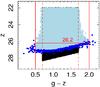 |
Fig. 5 Color–magnitude diagram of added stars. Black points: input values; dark-blue points: all recovered objects; light-blue points: applying same constraints as for selection of GC sample for ESO 306-017. |
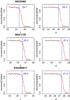 |
Fig. 6 Completeness tests. The dots are the fraction of recovered artificial stars as a function of magnitude. The solid red line in each panel shows the fitted Pritchet function. The blue line and number indicate where the data are nearly 100% complete. |
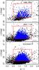 |
Fig. 7 Color–magnitude diagram of objects in the FG fields. The black dots are all the detected objects in the FOV. The thick gray lines show the error bars in color at different magnitudes. The blue dots framed within the red lines are the selected sample of GC candidates with color range 0.5 < g − z < 2.0. The bright magnitude limit is at |

As mentioned before, some contamination is expected due to foreground stars and unresolved background galaxies. To estimate the number of these contaminants, Ncont, the above detection procedure and selection criteria were applied to three “blank” background fields obtained from the HST archive that were chosen to have Galactic latitudes and exposure times in g and z similar to our two deeper fields (NGC 1132 andESO 306-017), but without any large galaxies present in the FOV.
To simulate the same detection conditions for the empty fields, we applied the rms maps of the FG fields to the background fields. The number of contaminants is taken to be the average of the three fields. We find Ncont = 7, 6 and 7 for NGC 6482, NGC 1132, and ESO 306-017, respectively; these values correspond to ~1% or less of the number of detected GC candidates, which is negligible. We note that NGC 6482 has Galactic latitude b ≈ 23°, about 10° less than that of the lowest latitude control field. Thus, its contamination may be somewhat higher, but not more than the few per cent level, as supported by the steep spatial distribution found below for the GC candidates in this galaxy.
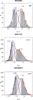 |
Fig. 8 Color histograms with the best GMM two-Gaussian fit. The individual Gaussians with their mean value are indicated with a blue or red number and solid curve; their sum is the black solid line. The hatched areas indicate the objects we include in the blue and red populations. The number of GCs is shown in the upper right of each panel. |
3. Analysis and results
3.1. Globular cluster color distribution
To detect and quantify the existence of color bimodality, the data were binned in (g − z) using an optimum bin size, Bopt (Izenman 1991; Peng et al. 2006), that depends on the sample size, n, and inter-quartile range, IQR which is a measure of the dispersion of the distribution:  (3)Afterwards, we used the algorithm Gaussian mixture modeling (GMM), which identifies Gaussian distributions with different parameters inside a dataset through the expectation maximization (EM) algorithm (Muratov & Gnedin 2010). GMM also performs independent tests of bimodality (measure of means separation and kurtosis), estimates the error of each parameter with bootstrapping, and estimates the confidence level at which a unimodal distribution can be rejected.
Figure 8 shows the (g − z) color distributions with the best fit Gaussians obtained with GMM. For NGC 6482 the best model is homoscedastic (same variance), while for NGC 1132 and ESO 306-017, a heteroscedastic (different variance) model provides a significantly better fit. The means, μcolor, and dispersions, σcolor, of the best fitting Gaussians are listed in Table 3; they are consistent with parameters in the literature (Peng et al. 2006). In Table 3, Cols. 9 and 10 we list the probability of obtaining the recovered values from a unimodal Gaussian distribution. Since these probabilities are small we are confident that the color distributions are bimodal relative to a null hypothesis of Gaussian unimodality.
3.2. Globular cluster spatial distribution
Harris (1991) noted that in general the GC systems are more extended than the starlight in their parent galaxies. Furthermore, it is known that the blue and red GCs have different spatial distribution, where the blue GCs have a more extended distribution than the red GCs (Geisler et al. 1996; Rhode & Zepf 2004). To see how the distributions compare in these FGs, we first need to select the blue and red GC subsamples.
In Fig. 8, we see that the two Gaussian components of the color distributions overlap; to avoid cross-contamination between the two populations, we reject objects in the overlapped regions, selecting blue and red population as indicated by the hatched regions. Because the mixed fraction are different for the three FGs color distributions, the cuts are different for each one: μblue + 0.1 for NGC 6482 and μblue for NGC 1132 and ESO 306-017; μred − 0.1 for NGC 6482 and NGC 1132 and μred for ESO 306-017 (see Fig. 8). Figure 9 shows the spatial distribution of blue and red GCs thus defined.
Parameters of the best GMM fit.
We measured the surface number density N of the blue and red populations by counting the number of GCs inside circular annuli with a width of  150 pixels. To compare the GC spatial distribution with the starlight profiles, we fitted Sérsic functions to the radial N profiles. The fitted function is:
 ![Mathematical equation: \begin{equation} N(r)= N_0\exp\left\{-b_n \left[ {\left( \frac{r}{{R_{\rm e}}^{\rm GC}}\right) }^{1/n_{\rm GC}}- 1\right] \right\} \end{equation}](/articles/aa/full_html/2012/10/aa19285-12/aa19285-12-eq135.png) (4)where
(4)where  is the effective radius, that contains half of the GC population; N0 is the surface number density at , nGC is the Sérsic index. We performed a second fit excluding the innermost point since the GCs closest to the galaxy center are more strongly affected by dynamical friction. In Fig. 10, we show the density profiles of all, blue, and red GCs, together with the best Sérsic fits. Table 4 shows the fitted parameters. As expected, the difference between both fits is larger for the closest system, NGC 6482 because we are looking at smaller physical scales than for NGC 1132 and ESO 306-017.
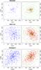 |
Fig. 9 Spatial distribution of blue and red populations selected from the color histograms (hatched regions in Fig. 8). Along with the red population, green ellipses show the starlight distribution. |
To compare the Sérsic profiles of the galaxy light (Fig. 10) with the GC number density (Fig. 2), in Fig. 11, we plot them together using an arbitrary relative scale. From this plot we can see that the GC distribution in each galaxy is more extended than its starlight. Nevertheless, we must remember that the comparison of Re is accurate only if the profiles have similar n.
We find that  is larger than
  , and Figs. 9 and 10 show that the blue populations are more extended than the red ones for these three FGs. Also, the distribution of the red populations are more elongated and seem to trace the shape of the galaxy.
3.3. Globular cluster luminosity function
To parameterize the GCLF, the GC magnitudes, m, were binned, again using an optimum bin size (Eq. (3)). Figure 12 show the GCLFs for NGC 6482, NGC 1132, and ESO 306-017, respectively. Because we are photometrically limited, we do not detect all the GCs in the FOV. The GCLFs that we recover are the convolution of the intrinsic GCLFs and the incompleteness functions. To get the total number of GCs in the FOV,  , we fit the product of a Gaussian and a Pritchet function to the GC magnitudes. The function we fit is:
 ![Mathematical equation: \begin{equation} f(m)=\frac{a_0}{\sqrt{2\pi\sigma_{\rm GCLF}^2}}{\rm e}^{\frac{-(m-m^0)}{2\sigma_{\rm GCLF}^2}}* \frac{1}{2}\left[1-\frac{\alpha(m-m_{\rm lim})}{\sqrt{1+\alpha^2(m-m_{\rm lim})^2}}\right]\cdot \end{equation}](/articles/aa/full_html/2012/10/aa19285-12/aa19285-12-eq143.png) (5)The values of the parameters α and mlim are obtained from the incompleteness test. We perform two fits. Firstly, we treat the mean value, m0, and amplitude, a0, of the Gaussian as free parameters, and fix the dispersion of the Gaussian to σGCLF = 1.4 (Jordán et al. 2006). Secondly, we fit for σGCLF and a0, and set m0. The fits were done by χ2 minimization using the Optim task (described in Sect. 2.1). The same procedure was performed independently in g and z band, obtaining better results in z band and fixing σGCLF. Table 5 shows the best fit values for σGCLF and m0 recovered and their estimated , respectively. From Fig. 12 we can see that the recovered values are consistent with the expected values for NGC 1132 and ESO 306-017, however for NGC 6482 the recovered m0 and σGCLF are shifted by ~ 0.5 and 0.2, respectively.
(5)The values of the parameters α and mlim are obtained from the incompleteness test. We perform two fits. Firstly, we treat the mean value, m0, and amplitude, a0, of the Gaussian as free parameters, and fix the dispersion of the Gaussian to σGCLF = 1.4 (Jordán et al. 2006). Secondly, we fit for σGCLF and a0, and set m0. The fits were done by χ2 minimization using the Optim task (described in Sect. 2.1). The same procedure was performed independently in g and z band, obtaining better results in z band and fixing σGCLF. Table 5 shows the best fit values for σGCLF and m0 recovered and their estimated , respectively. From Fig. 12 we can see that the recovered values are consistent with the expected values for NGC 1132 and ESO 306-017, however for NGC 6482 the recovered m0 and σGCLF are shifted by ~ 0.5 and 0.2, respectively.
3.4. Specific frequency
As noted previously, the specific frequency SN is the number of GCs per unit galaxy luminosity, defined such that  (6)where NGC is the number of GCs, MV is the absolute magnitude of the galaxy in V band, and both quantities measured over the same area. Although the parameters recovered from the GCLF fitting are consistent with expectations for NGC 1132 and ESO 306-017, they are not for NGC 6482. Thus, to estimate SN we use the expected turnover magnitudes (Col. 10 in Table 1) and fix σGCLF = 1.4 to calculate more conservative values of the total GC number,
  , for the three FGs. Although we do not fit for the GCLF parameters in this case, our error estimates for the total GC number include a contribution arising from the uncertainties in the GCLF parameters. The resulting values of and their uncertainties are listed in Col. 2 of Table 6 and are generally consistent with the values estimated previously as part of the GCLF analysis in Sect. 3.3.
Calculation of the specific frequency also requires knowledge of the galaxy luminosity. To estimate the absolute V-band magnitudes of the galaxies, we first calculate the g and z magnitudes from the counts in our 2D isophotal model images, subtracting the sky values estimated from the Sérsic fits. Then, we apply the transformation V = g + 0.320 − 0.399(g − z) given by Kormendy et al. (2009).
The specific frequencies and absolute magnitudes in the g, z and V bandpasses within the FOV are listed in Table 6. Both the GC population size and the SN increase with the galaxy luminosity for these three FGs. There is a range of more than a factor of 3 in SN, from ≲ 2 for NGC 6482 to ≳ 6 forESO 306-017. This spans the full range of values for normal bright ellipticals in the Virgo cluster, as we discuss in the following section.
We note that these results are largely independent of the galaxy profile fits, which are mainly used for estimating the sky background. In particular, although the unusually high Sérsic index n ≈ 11 for ESO 306-017 could in part result from the limited spatial range of the fitted profile, this would not affect the SN, as we do not directly use the Sérsic fit to calculate the galaxy luminosity. Sun et al. (2004) found from much lower resolution ground-based imaging that the n value is lower forESO 306-017 at radii beyond the ACS FOV. Adopting a Sérsic profile with a lower n would result in a larger sky estimate, slightly decreasing the luminosity estimate and increasing the SN value. However, if our estimated profile is accurate within the FOV, the estimated sky and SN should also be accurate.
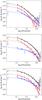 |
Fig. 10 Surface number density of GCs. The dots are the data and the lines show the best Sérsic fits including all the points (dashed lines) and excluding the innermost point (solid lines) for all the GCs detected (black), only blue GCs (blue), and only red GCs (red). Top to bottom: NGC 6482, NGC 1132 and ESO 306-017. |
Finally, we could extrapolate the GC radial density profiles and the galaxy surface brightness fits to estimate “global” SN values, but the extrapolated galaxy profiles are very sensitive to the sky levels, which we cannot measure directly for our larger galaxies. Moreover, as noted above, there is evidence from the literature that an extrapolation of our Sérsic fit forESO 306-017 would not accurately describe its outer profile. The GC number density profiles in Fig. 10 also become very uncertain at large radii. We therefore opt to report the more reliable, directly observed, values within the FOV. The general tendency of GC systems to be more extended than the galaxy light means that the global SN might be slightly higher.
4. Discussion
4.1. Comparison with cluster ellipticals
One of the most basic questions to address is whether the GC systems in these FG ellipticals differ from those of cluster ellipticals. To compare our results with the literature, we chose the ACS Virgo Cluster Survey (ACSVCS) sample of 100 early-type galaxies (Côté et al. 2004), comprising the largest and most homogeneous data set on the GC populations of cluster early-type galaxies. Moreover, the observations were taken with the same instrument and filters as the current study. The ACS Fornax Cluster Survey (Jordán et al. 2007a) targeted a sample of early-type galaxies in Fornax, but the complete results on the GC systems remain to be published. Cho et al. (2012) studied the GC systems in a smaller sample of elliptical galaxies in low-density environments, but the results were generally similar to those found for galaxies in Virgo.
GC surface density Sérsic parameters for all, red and blue populations.
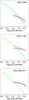 |
Fig. 11 Comparison of Sérsic profiles of the galaxy in the z band (green line), and of the surface number density of blue (blue line) and red (red line) GC populations, excluding the inner point in the fit. The relative scale of the galaxy and GC profiles is arbitrary. Top to bottom: NGC 6482, NGC 1132 and ESO 306017. |
Peng et al. (2006) found that the GC color distributions of the bright ACSVCS galaxies were essentially all bimodal, with both the red and blue peaks becoming redder for more luminous galaxies. Likewise, we find that the color distributions of the GCs in all three of our FG galaxies are bimodal. Given the small size of our sample and the large scatters in the relations between GC peak colors and galaxy luminosity, our measurements are generally consistent with those Peng et al. (2006). However, one surprising result is that the lowest luminosity FG galaxy NGC 6482 actually has the reddest mean GC color, ⟨ g − z ⟩ = 1.26 mag, equal to that of NGC 4649 (M60), the ACSVCS galaxy with the reddest mean GC color. We discuss this further in the following section.
The specific frequencies of the ACSVCS galaxies, and the implications for formation efficiencies, were investigated in detail by Peng et al. (2008). Even though the FOV encloses different physical scales due to different distances of the Virgo cluster and our FG galaxies, most of the ACSVCS galaxies are small enough to encompass the entire GC system in the FOV, while for the largest galaxies, an extrapolated value to large radius was reported. Although SN tends to increase with luminosity among giant ellipticals, the mean SN attains a minimum value of ~2 for early-type galaxies with MV ≈ − 20, then increases again, but with much larger scatter, at lower luminosities. Figure 13 (right panel) shows that the three FGs studied here follow the trend defined by the most luminous members of the 100 early-type ACSVCS galaxies. In particular, ESO 306-017 has the highest luminosity in the combined sample, and its value of SN = 6.3 is greater than that of all other 50 + galaxies with MV < −18 except for M 87, which is the extreme high-SN outlier in this plot. The left panel of Fig. 13 shows that the FGs also follow the tendency of higher luminosity ellipticals to have larger Sérsic indices (Ferrarese et al. 2006). Thus, it appears that the FG galaxies accord well with the general SN and surface brightness trends of normal giant ellipticals, and lack (at least in this limited sample) the anomalously large SN values seen in some cD galaxies such as M 87.
4.2. Comparisons with X-ray data
The definition of FG includes a minimum X-ray luminosity, thus, if an object is classified as FG, it must be detected in X-rays. It has been noted that the X-ray luminosities of the extended haloes of FGs are similar those of the intracluster media in galaxy clusters (Mendes de Oliveira et al. 2009; Fasano et al. 2010). For each FG studied here, we show in Table 7 the literature values for its X-ray luminosity, metal abundance of the intra-group gas, and M/L determined from X-ray data.
For NGC 6482, the luminosity was obtained from Khosroshahi et al. (2004) who analyzed Chandra data. They also noted a central point source, possibly an AGN. Yoshioka et al. (2004) analyzed ASCA data for NGC 1132 and classified it as an “isolated X-ray overluminous elliptical galaxy” (IOLEG). For ESO 306-017, we use the results from Sun et al. (2004), who analyzed Chandra and XMM-Newton data and averaged the results of these analyses. They also noted an X-ray finger emanating from the central X-ray peak to the brightest companion galaxy, similar in location to the tidal feature reported in the present study (see Sect. 2.1). The X-ray emission of this finger is 20–30% brighter than other regions at the same radius.
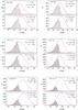 |
Fig. 12 GC luminosity functions in the g (left panel) and z (right panel) bands. The dashed lines show the best-fit Gaussian × Pritchet (completeness function) model, and the solid lines are the respective Gaussians. The numbers indicate the fixed and fitted parameters. Top to bottom: NGC 6482, NGC 1132 and ESO 306-017. |
Table 7 includes the literature values of the M/Ls. However, we must be cautious in comparing these values because of different assumptions made by different authors, mainly regarding the optical luminosity and because of the large uncertainties in mass estimates (see Khosroshahi et al. 2007, discussion). For instance, Yoshioka et al. (2004) assumed a much lower contribution for the non-brightest galaxies to the total optical luminosity, compared with Khosroshahi et al. (2006) and Sun et al. (2004), a fact that increases their M/L estimate. Thus, systematic uncertainties can make it difficult to determine whether or not there is any trend in GC properties with M/L.
While three objects are an insufficient sample for drawing general conclusions, we do see hints of interesting trends when comparing the properties of the X-ray gas and GC systems (Table 3). The results are consistent with positive correlations between X-ray luminosity, GC number, and SN, similar to the trends found for BCGs (e.g., Blakeslee 1999; West et al. 1995). There may also be a trend with optical luminosity. Intriguingly, the mean color of the GC population ( ⟨ g − z ⟩ = 1.26, 1.11 and 1.20 for NGC 6482, NGC 1132 and ESO 306-017, respectively) becomes redder as the metal abundance of the intra-group gas increases. The apparent correlations of the properties of the GC systems with X-ray intra-group gas abundance and galaxy luminosity suggest that these components might likely formed at similar epochs.
One might expect the systems with the highest X-ray luminosities and masses to possess the most metal-rich GC systems, but this is apparently not the case for this small sample of FGs. The mean color of the GC system does not correlate with X-ray luminosity, but interestingly, it does with X-ray metallicity. This could be an indication that the metal enrichment is not set mainly by the mass but by the concentration of the halo (Atlee & Martini 2012). The dark matter concentration, c, is measured as the ratio of the virial radius to the radius of a sphere enclosing 0.2 the virial mass (von Benda-Beckmann et al. 2008). Higher c values are associated with an earlier formation epoch (Khosroshahi et al. 2007; von Benda-Beckmann et al. 2008). Numerical simulations indicate that FGs have higher values of c than galaxy groups with similar masses but not classified as FGs (c = 6.4 for FGs and c = 5.5 for normal groups). The c values reported for NGC 6482, NGC 1132 and ESO 306-017 are 60, 38 and 8.5 (see Fig. 9 from Khosroshahi et al. 2007); all of these are high, with the value for NGC 6482 being quite extreme. However, the dark matter concentration on these scales is notoriously difficult to constrain observationally.
High concentrations can help fuel larger rates of star-formation, producing a higher proportion of massive stellar systems such as GCs (Larsen & Richtler 2000; Peng et al. 2008), as well as making self-enrichment more efficient. Thus, the possible link between dark matter halo concentration, X-ray gas metallicity, and GC mean color may be understood in the context of early and violent dissipative assembly, whereby a first generation of GCs contaminate the surrounding media from which the bulk of the stars formed. Eventually the feedback from star formation (and possibly AGN) heats the gas and suppresses subsequent star formation (see Johansson et al. 2012). Afterwards, the galaxy continues growing by non-dissipative minor mergers (De Lucia et al. 2006; Naab et al. 2009). Of course, a larger sample of FGs is needed to confirm these correlations before drawing more detailed conclusions on the star formation histories of FG galaxies.
GCLF fitted parameters.
Specific frequency.
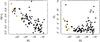 |
Fig. 13 Fossil groups in context: galaxy Sérsic index (left) and SN are plotted as a function of MV for the fossil groups studied here (orange triangles) and the ACS Virgo Cluster Survey galaxies (black circles). The Virgo data are from Ferrarese et al. (2006) and Peng et al. (2008). |
5. Conclusions
The main results of this study are:
-
1.
We detected 369, 1410 and 1918 GCs down to mag-nitude z = 24.7, 26.2 and 26.2 in NGC 6482,NGC 1132 and ESO 306-017, respectively; after completeness correction and assuminga Gaussian GCLF with expected
 and σGCLF = 1.4, the number of GCs ineach FOV are: 1140 ± 87,3613 ± 295 and 11[en-tity!#x2009!]577 ± 1046,respectively.
 -
2.
The GC color distributions for all three FGs are better described by a bimodal, rather than unimodal Gaussian model. For the heteroscedastic cases, NGC 1132 and ESO 306-017, the dispersion of the red population is wider than the blue. The mean g − z colors are: 1.26, 1.11 and 1.20 for NGC 6482, NGC 1132 and ESO 306-017, respectively. The mean color for NGC 6482 is unusually red; it is interesting that this is also the FG with the highest X-ray gas metallicity.
-
3.
For all three FGs, the spatial distribution of the starlight is more concentrated than that of the GCs, and the blue GCs are more extended than the red ones, similar to the case for other ellipticals.
-
4.
The derived values of SN are: 1.9 ± 0.1, 3.1 ± 0.3 and 6.3 ± 0.6 for NGC 6482, NGC 1132 and ESO 306-017, respectively. These span the full range for normal ellipticals in the Virgo cluster. The results are consistent with both the total number of GCs and SN increasing with the optical luminosity of the galaxy and the X-ray luminosity from the intra-group gas.
-
5.
From analysis of the surface brightness distributions, we found evidence of recent interactions, particularly in ESO 306-017, which shows a tidal feature coincident with the finger reported previously in X-rays, and NGC 1132, which has shell-like structure. While NGC 6482 is well-described by a standard Sérsic profile, the two brighter galaxies are better fitted by core-Sérsic models. All three galaxies contain central dust features. These observations are consistent with numerical simulations indicating that signs of recent merging should be fairly common in first-ranked FG galaxies (Díaz-Giménez et al. 2008), and they suggest that the paradigm of FGs as relaxed, undisturbed systems needs to be reconsidered.
X-ray properties.
Larger samples of GC systems in FGs are needed to make more definite conclusions. However, overall we conclude that the GC properties (colors, spatial distributions, specific frequencies) in FG central galaxies are generally similar to those seen in other giant ellipticals, which mainly reside in clusters. Although the environments differ, this study suggests that the GC systems formed under very similar conditions. These results might therefore be taken as a confirmation that the same basic formation processes are responsible for the buildup of massive early-type galaxies in all environments.
STSDAS is a product of the Space Telescope Science Institute, which is operated by AURA for NASA.
SExtractor parameter that classifies the objects according to their fuzziness; point sources have CLASS_STAR ~ 1, while for extended objects it is ~ 0.
Acknowledgments
We thank the anonymous referee for his/her helpful comments and suggestions that helped to improve the clarity of the manuscript. A.J. acknowledges support from Ministry of Economy ICM Nucleus P07-021-F, Anillo ACT-086 and BASAL CATA PFB-06. K.A.A.-M. acknowledges the support of ESO through a studenship and CONACyT (Mexico). Support for program #10558 was provided by NASA through a grant from the Space Telescope Science Institute, which is operated by the Association of Universities for Research in Astronomy, Inc., under NASA contract NAS 5-26555.
References
- Atlee, D. W., & Martini, P. 2012, ApJ, submitted [arXiv:1201.2957] [Google Scholar]
- Bertin, E., & Arnouts, S. 1996, A&AS, 117, 393 [NASA ADS] [CrossRef] [EDP Sciences] [Google Scholar]
- Blakeslee, J. P. 1999, AJ, 118, 1506 [NASA ADS] [CrossRef] [Google Scholar]
- Blakeslee, J. P., Tonry, J. L., & Metzger, M. R. 1997, AJ, 114, 482 [NASA ADS] [CrossRef] [Google Scholar]
- Blakeslee, J. P., Anderson, K. R., Meurer, G. R., et al. 2003, Astronomical Data Analysis Software and Systems XII, 295, 257 [Google Scholar]
- Blakeslee, J. P., Cho, H., Peng, E. W., et al. 2012, ApJ, 746, 88 [NASA ADS] [CrossRef] [Google Scholar]
- Brodie, J. P., & Huchra, J. P. 1991, ApJ, 379, 157 [NASA ADS] [CrossRef] [Google Scholar]
- Brodie, J. P., & Strader, J. 2006, ARA&A, 44, 193 [NASA ADS] [CrossRef] [Google Scholar]
- Byun, Y.-I., Grillmair, C. J., Faber, S. M., et al. 1996, AJ, 111, 1889 [NASA ADS] [CrossRef] [Google Scholar]
- Chies-Santos, A. L., Larsen, S. S., Cantiello, M., et al. 2012, A&A, 539, A54 [NASA ADS] [CrossRef] [EDP Sciences] [Google Scholar]
- Cho, J., Sharples, R. M., Blakeslee, J. P., et al. 2012, MNRAS, 422, 3591 [NASA ADS] [CrossRef] [Google Scholar]
- Cohen, J. G., & Côté, P. 2003, ApJ, 592, 866 [NASA ADS] [CrossRef] [Google Scholar]
- Cohen, J. G., Blakeslee, J. P., & Ryzhov, A. 1998, ApJ, 496, 808 [NASA ADS] [CrossRef] [Google Scholar]
- Côté, P., Marzke, R. O., & West, M. J. 1998, ApJ, 501, 554 [NASA ADS] [CrossRef] [Google Scholar]
- Côté, P., Blakeslee, J. P., Ferrarese, L., et al. 2004, ApJS, 153, 223 [NASA ADS] [CrossRef] [Google Scholar]
- Côté, P., Ferrarese, L., Jordán, A., et al. 2007, ApJ, 671, 1456 [NASA ADS] [CrossRef] [Google Scholar]
- Cui, W., Springel, V., Yang, X., De Lucia, G., & Borgani, S. 2011, MNRAS, 416, 2997 [NASA ADS] [CrossRef] [Google Scholar]
- Cypriano, E. S., Mendes de Oliveira, C. L., & Sodré, L., Jr. 2006, AJ, 132, 514 [NASA ADS] [CrossRef] [Google Scholar]
- Dariush, A., Khosroshahi, H. G., Ponman, T. J., et al. 2007, MNRAS, 382, 433 [NASA ADS] [CrossRef] [Google Scholar]
- De Lucia, G., Springel, V., White, S. D. M., Croton, D., & Kauffmann, G. 2006, MNRAS, 366, 499 [NASA ADS] [CrossRef] [Google Scholar]
- D’Onghia, E., Sommer-Larsen, J., Romeo, A. D., et al. 2005, ApJ, 630, L109 [NASA ADS] [CrossRef] [Google Scholar]
- Díaz-Giménez, E., Muriel, H., & Mendes de Oliveira, C. 2008, A&A, 490, 965 [NASA ADS] [CrossRef] [EDP Sciences] [Google Scholar]
- Díaz-Giménez, E., Zandivarez, A., Proctor, R., Mendes de Oliveira, C., & Abramo, L. R. 2011, A&A, 527, A129 [NASA ADS] [CrossRef] [EDP Sciences] [Google Scholar]
- Eigenthaler, P., & Zeilinger, W. W. 2012, A&A, 540, A134 [NASA ADS] [CrossRef] [EDP Sciences] [Google Scholar]
- Fall, S. M., & Rees, M. J. 1985, ApJ, 298, 1 [NASA ADS] [CrossRef] [Google Scholar]
- Fasano, G., Bettoni, D., Ascaso, B., et al. 2010, MNRAS, 404, 1490 [NASA ADS] [Google Scholar]
- Ferrarese, L., Côté, P., Jordán, A., et al. 2006, ApJS, 164, 334 [NASA ADS] [CrossRef] [Google Scholar]
- Fleming, D. E. B., Harris, W. E., Pritchet, C. J., & Hanes, D. A. 1995, AJ, 109, 1044 [NASA ADS] [CrossRef] [Google Scholar]
- Forbes, D. A., Franx, M., Illingworth, G. D., & Carollo, C. M. 1996, ApJ, 467, 126 [NASA ADS] [CrossRef] [Google Scholar]
- Forbes, D. A., Brodie, J. P., & Huchra, J. 1997, AJ, 113, 887 [NASA ADS] [CrossRef] [Google Scholar]
- Gebhardt, K., & Kissler-Patig, M. 1999, AJ, 118, 1526 [NASA ADS] [CrossRef] [Google Scholar]
- Geisler, D., Lee, M. G., & Kim, E. 1996, AJ, 111, 1529 [NASA ADS] [CrossRef] [Google Scholar]
- Graham, A. W., & Driver, S. P. 2005, PASA, 22, 118 [NASA ADS] [CrossRef] [Google Scholar]
- Graham, A., Lauer, T. R., Colless, M., & Postman, M. 1996, ApJ, 465, 534 [NASA ADS] [CrossRef] [Google Scholar]
- Harris, W. E. 1991, AJ, 102, 1348 [NASA ADS] [CrossRef] [Google Scholar]
- Harris, W. E. 1991, ARA&A, 29, 543 [NASA ADS] [CrossRef] [Google Scholar]
- Harris, W. E., & van den Bergh, S. 1981, AJ, 86, 1627 [NASA ADS] [CrossRef] [Google Scholar]
- Harris, W. E., & Harris, G. L. H. 2002, AJ, 123, 3108 [NASA ADS] [CrossRef] [Google Scholar]
- Izenman, A. J. 1991, Am. Stat. Assoc., 86, 205 [Google Scholar]
- Jedrzejewski, R. I. 1987, MNRAS, 226, 747 [Google Scholar]
- Johansson, P. H., Naab, T., & Ostriker, J. P. 2012, ApJ, 754, 115 [NASA ADS] [CrossRef] [Google Scholar]
- Jones, L. R., Ponman, T. J., Horton, A., et al. 2003, MNRAS, 343, 627 [NASA ADS] [CrossRef] [Google Scholar]
- Jordán, A., Côté, P., West, M. J., et al. 2004, AJ, 127, 24 [NASA ADS] [CrossRef] [Google Scholar]
- Jordán, A., Côté, P., Blakeslee, J. P., et al. 2005, ApJ, 634, 1002 [NASA ADS] [CrossRef] [Google Scholar]
- Jordán, A., McLaughlin, D. E., Côté, P., et al. 2006, ApJ, 651, L25 [NASA ADS] [CrossRef] [Google Scholar]
- Jordán, A., McLaughlin, D. E., Côté, P., et al. 2007a, ApJS, 171, 101 [NASA ADS] [CrossRef] [Google Scholar]
- Jordán, A., Blakeslee, J. P., Côté, P., et al. 2007b, ApJS, 169, 213 [NASA ADS] [CrossRef] [Google Scholar]
- Khosroshahi, H. G., Jones, L. R., & Ponman, T. J. 2004, MNRAS, 349, 1240 [NASA ADS] [CrossRef] [Google Scholar]
- Khosroshahi, H. G., Ponman, T. J., & Jones, L. R. 2006, MNRAS, 372, L68 [NASA ADS] [CrossRef] [Google Scholar]
- Khosroshahi, H. G., Ponman, T. J., & Jones, L. R. 2007, MNRAS, 377, 595 [NASA ADS] [CrossRef] [Google Scholar]
- Kormendy, J., Fisher, D. B., Cornell, M. E., & Bender, R. 2009, ApJS, 182, 216 [NASA ADS] [CrossRef] [Google Scholar]
- La Barbera, F., Paolillo, M., De Filippis, E., & de Carvalho, R. R. 2012, MNRAS, 422, 3010 [NASA ADS] [CrossRef] [Google Scholar]
- Larsen, S. S., & Richtler, T. 2000, A&A, 354, 836 [NASA ADS] [Google Scholar]
- Madrid, J. P. 2011, ApJ, 737, L13 [NASA ADS] [CrossRef] [Google Scholar]
- McLaughlin, D. E., & Fall, S. M. 2008, ApJ, 679, 1272 [NASA ADS] [CrossRef] [Google Scholar]
- Mendes de Oliveira, C. L., & Carrasco, E. R. 2007, ApJ, 670, L93 [NASA ADS] [CrossRef] [Google Scholar]
- Mendes de Oliveira, C. L., Cypriano, E. S., Dupke, R. A., & Sodré, L., Jr. 2009, AJ, 138, 502 [NASA ADS] [CrossRef] [Google Scholar]
- Méndez-Abreu, J., Aguerri, J. A. L., Barrena, R., et al. 2012, A&A, 537, A25 [NASA ADS] [CrossRef] [EDP Sciences] [Google Scholar]
- Muratov, A. L., & Gnedin, O. Y. 2010, ApJ, 718, 1266 [NASA ADS] [CrossRef] [Google Scholar]
- Naab, T., Johansson, P. H., & Ostriker, J. P. 2009, ApJ, 699, L178 [NASA ADS] [CrossRef] [Google Scholar]
- Nair, P., van den Bergh, S., & Abraham, R. G. 2011, ApJ, 734, L31 [NASA ADS] [CrossRef] [Google Scholar]
- Nelder, J. A., & Mead, R. 1965, The Comput. J., 308, 313 [Google Scholar]
- Peng, E. W., Jordán, A., Côté, P., et al. 2006, ApJ, 639, 95 [NASA ADS] [CrossRef] [Google Scholar]
- Peng, E. W., Jordán, A., Côté, P., et al. 2008, ApJ, 681, 197 [NASA ADS] [CrossRef] [Google Scholar]
- Ponman, T. J., Allan, D. J., Jones, L. R., et al. 1994, Nature, 369, 462 [NASA ADS] [CrossRef] [Google Scholar]
- Postman, M., & Lauer, T. R. 1995, ApJ, 440, 28 [NASA ADS] [CrossRef] [Google Scholar]
- Press, W. H., & Schechter, P. 1974, ApJ, 187, 425 [NASA ADS] [CrossRef] [Google Scholar]
- Proctor, R. N., de Oliveira, C. M., Dupke, R., et al. 2011, MNRAS, 418, 2054 [NASA ADS] [CrossRef] [Google Scholar]
- Puzia, T. H., Kissler-Patig, M., Thomas, D., et al. 2005, A&A, 439, 997 [NASA ADS] [CrossRef] [EDP Sciences] [Google Scholar]
- Rhode, K. L., & Zepf, S. E. 2004, AJ, 127, 302 [NASA ADS] [CrossRef] [Google Scholar]
- Sales, L. V., Navarro, J. F., Theuns, T., et al. 2012, MNRAS, 423, 1544 [NASA ADS] [CrossRef] [Google Scholar]
- Sérsic, J. L. 1968, Atlas de Galaxias Australes (Cordoba: Observatorio Astronomico) [Google Scholar]
- Schlegel, D. J., Finkbeiner, D. P., & Davis, M. 1998, ApJ, 500, 525 [NASA ADS] [CrossRef] [Google Scholar]
- Schombert, J., & Smith, A. K. 2012 [arXiv:1203.2578] [Google Scholar]
- Sirianni, M., Jee, M. J., Benítez, N., et al. 2005, PASP, 117, 1049 [NASA ADS] [CrossRef] [Google Scholar]
- de Souza, R. E., Gadotti, D. A., & dos Anjos, S. 2004, ApJS, 153, 411 [NASA ADS] [CrossRef] [Google Scholar]
- Stetson, P. B. 1987, PASP, 99, 191 [NASA ADS] [CrossRef] [Google Scholar]
- Sun, M., Forman, W., Vikhlinin, A., et al. 2004, ApJ, 612, 805 [NASA ADS] [CrossRef] [Google Scholar]
- Tody, D. 1986, Proc. SPIE, 627, 733 [NASA ADS] [CrossRef] [Google Scholar]
- Tovmassian, H. 2010, Rev. Mex. Astron. Astrofis., 46, 61 [NASA ADS] [Google Scholar]
- Trujillo, I., Erwin, P., Asensio Ramos, A., & Graham, A. W. 2004, AJ, 127, 1917 [NASA ADS] [CrossRef] [Google Scholar]
- van den Bergh, S. 1975, ARA&A, 13, 217 [NASA ADS] [CrossRef] [Google Scholar]
- Vikhlinin, A., McNamara, B. R., Hornstrup, A., et al. 1999, ApJ, 520, L1 [NASA ADS] [CrossRef] [Google Scholar]
- Villegas, D., Jordán, A., Peng, E. W., et al. 2010, ApJ, 717, 603 [NASA ADS] [CrossRef] [Google Scholar]
- von Benda-Beckmann, A. M., D’Onghia, E., Gottlöber, S., et al. 2008, MNRAS, 386, 2345 [NASA ADS] [CrossRef] [Google Scholar]
- West, M. J., Cote, P., Jones, C., Forman, W., & Marzke, R. O. 1995, ApJ, 453, L77 [NASA ADS] [CrossRef] [Google Scholar]
- West, M. J., Côté, P., Marzke, R. O., & Jordán, A. 2004, Nature, 427, 31 [NASA ADS] [CrossRef] [PubMed] [Google Scholar]
- Yoon, S.-J., Yi, S. K., & Lee, Y.-W. 2006, Science, 311, 1129 [NASA ADS] [CrossRef] [PubMed] [Google Scholar]
- Yoon, S.-J., Lee, S.-Y., Blakeslee, J. P., et al. 2011, ApJ, 743, 150 [NASA ADS] [CrossRef] [Google Scholar]
- Yoshioka, T., Furuzawa, A., Takahashi, S., et al. 2004, Adv. Space Res., 34, 2525 [NASA ADS] [CrossRef] [Google Scholar]
- Zepf, S. E., & Ashman, K. M. 1993, MNRAS, 264, 611 [NASA ADS] [CrossRef] [Google Scholar]
- Zinn, R. 1985, ApJ, 293, 424 [Google Scholar]
All Tables
Best galaxy surface brightness model parameters in g and z bands: single Sérsic for NGC 6484 and core-Sérsic for NGC 1132 and ESO 306-017.
All Figures
|
Fig. 1 ACS color images, FOV |
| In the text | |
|
Fig. 2 Galaxy surface brightness distribution as a function of the isophotal equivalent circular radius Rc. The dots are the data after subtraction of the fitted sky value. The solid red lines show the best fit profiles: single Sérsic for NGC 6482 and core-Sérsic for NGC 1132 and ESO 306-017. For the galaxies where the best fit is core-Sérsic, the dashed blue line shows the single Sérsic. Top to bottom: NGC 6482, NGC 1132 and ESO 306-017. The left and right panels are the g and z band, respectively. For ESO 306-017, the gray dots were not included in the fit. |
| In the text | |
|
Fig. 3 Residual images after subtracting the best single Sérsic model, in z band: NGC 6482 (left), NGC 1132 (center), and ESO 306-017 (right). The galaxies are shown at the observed orientation. |
| In the text | |
|
Fig. 4 Inner regions of g-band images: NGC 6482 (left), NGC 1132 (center), and ESO 306-017 (right). Dust is present in all cases. |
| In the text | |
|
Fig. 5 Color–magnitude diagram of added stars. Black points: input values; dark-blue points: all recovered objects; light-blue points: applying same constraints as for selection of GC sample for ESO 306-017. |
| In the text | |
|
Fig. 6 Completeness tests. The dots are the fraction of recovered artificial stars as a function of magnitude. The solid red line in each panel shows the fitted Pritchet function. The blue line and number indicate where the data are nearly 100% complete. |
| In the text | |
|
Fig. 7 Color–magnitude diagram of objects in the FG fields. The black dots are all the detected objects in the FOV. The thick gray lines show the error bars in color at different magnitudes. The blue dots framed within the red lines are the selected sample of GC candidates with color range 0.5 < g − z < 2.0. The bright magnitude limit is at |
| In the text | |
|
Fig. 8 Color histograms with the best GMM two-Gaussian fit. The individual Gaussians with their mean value are indicated with a blue or red number and solid curve; their sum is the black solid line. The hatched areas indicate the objects we include in the blue and red populations. The number of GCs is shown in the upper right of each panel. |
| In the text | |
|
Fig. 9 Spatial distribution of blue and red populations selected from the color histograms (hatched regions in Fig. 8). Along with the red population, green ellipses show the starlight distribution. |
| In the text | |
|
Fig. 10 Surface number density of GCs. The dots are the data and the lines show the best Sérsic fits including all the points (dashed lines) and excluding the innermost point (solid lines) for all the GCs detected (black), only blue GCs (blue), and only red GCs (red). Top to bottom: NGC 6482, NGC 1132 and ESO 306-017. |
| In the text | |
|
Fig. 11 Comparison of Sérsic profiles of the galaxy in the z band (green line), and of the surface number density of blue (blue line) and red (red line) GC populations, excluding the inner point in the fit. The relative scale of the galaxy and GC profiles is arbitrary. Top to bottom: NGC 6482, NGC 1132 and ESO 306017. |
| In the text | |
|
Fig. 12 GC luminosity functions in the g (left panel) and z (right panel) bands. The dashed lines show the best-fit Gaussian × Pritchet (completeness function) model, and the solid lines are the respective Gaussians. The numbers indicate the fixed and fitted parameters. Top to bottom: NGC 6482, NGC 1132 and ESO 306-017. |
| In the text | |
|
Fig. 13 Fossil groups in context: galaxy Sérsic index (left) and SN are plotted as a function of MV for the fossil groups studied here (orange triangles) and the ACS Virgo Cluster Survey galaxies (black circles). The Virgo data are from Ferrarese et al. (2006) and Peng et al. (2008). |
| In the text | |
Current usage metrics show cumulative count of Article Views (full-text article views including HTML views, PDF and ePub downloads, according to the available data) and Abstracts Views on Vision4Press platform.
Data correspond to usage on the plateform after 2015. The current usage metrics is available 48-96 hours after online publication and is updated daily on week days.
Initial download of the metrics may take a while.