| Issue |
A&A
Volume 546, October 2012
|
|
|---|---|---|
| Article Number | A111 | |
| Number of page(s) | 12 | |
| Section | Extragalactic astronomy | |
| DOI | https://doi.org/10.1051/0004-6361/201218783 | |
| Published online | 17 October 2012 | |
Lyman-α emission properties of simulated galaxies: interstellar medium structure and inclination effects
1
Oxford Astrophysics, University of Oxford,
Denys Wilkinson Building, Keble
Road, Oxford,
OX1 3RH,
UK
2
Université de Lyon, 69003 Lyon, France Université Lyon 1,
Observatoire de Lyon, 9 avenue Charles André, 69230 Saint-Genis Laval, France CNRS,
UMR 5574, Centre de Recherche
Astrophysique de Lyon, École Normale Supérieure de Lyon,
69007
Lyon,
France
e-mail: anne.verhamme@univ-lyon1.fr
3
Institut d’Astrophysique de Paris, 98bis boulevard Arago, 75014
Paris,
France
4
Centre for Astrophysics & Supercomputing, Swinburne
University of Technology, PO Box
218, Hawthorn,
VIC
3122,
Australia
Received: 6 January 2012
Accepted: 21 August 2012
Aims. This paper is the first in a series investigating Lyman-alpha (hereafter Lyα) radiation transfer through hydrodynamical simulations of galaxy formation. Its aim is to assess the impact of interstellar medium (ISM) physics on Lyα radiation transfer and to quantify how galaxy orientation alters observational signatures with respect to the line of sight.
Methods. We compare the results of Lyα radiation transfer calculations through the ISM of a couple of idealized galaxy simulations in a dark matter halo of ~1010 M⊙. In the first one, G1, this ISM is modeled using physics typical of large-scale cosmological hydrodynamics simulations of galaxy formation, where gas is prevented from radiatively cooling below 104 K. In the second one, G2, gas is allowed to radiate away more of its internal energy via metal lines and consequently fragments into dense star-forming clouds.
Results. First, as expected, the small-scale structuration of the ISM plays a determinant role in shaping a galaxy’s Lyα properties. The artificially warm, hence smooth, ISM of G1 yields an escape fraction of ~50% at the Lyα line center, and produces symmetrical double-peak profiles. In contrast, in G2, most young stars are embedded in thick star-forming clouds, and the result is a ~10 times lower escape fraction. G2 also displays a stronger outflowing velocity field, which favors the escape of red-shifted photons, resulting in an asymmetric Lyα line. Second, the Lyα properties of G2 strongly depend on the inclination at which it is observed: From edge-on to face-on, the line goes from a double-peak profile with an equivalent width (EW) of ~−5 Å to a 15 times more luminous, red-shifted asymmetric line with EW ~ 90 Å.
Conclusions. The remarkable discrepancy in the Lyα properties we derived for two ISM models raises a fundamental question. In effect, it demonstrates that Lyα radiation transfer calculations can only lead to realistic properties in simulations where galaxies are resolved into giant molecular clouds. Such a stringent requirement translates into severe constraints both in terms of ISM physics modeling and numerical resolution, putting these calculations beyond the reach of current large-scale cosmological simulations. Finally, we find inclination effects to be much stronger for Lyα photons than for continuum radiation. This could potentially introduce severe biases in the selection function of narrow-band Lyα emitter surveys and in their interpretation, and we predict that these surveys could indeed miss a significant fraction of the high-z galaxy population.
Key words: methods: numerical / radiative transfer / hydrodynamics / galaxies: ISM / ISM: kinematics and dynamics / ISM: structure
© ESO, 2012
1. Introduction
In the past decade, the Lyman-alpha (Lyα) emission line has become an observational tool of choice for detecting high-redshift galaxies via narrow-band surveys (e.g. Hu et al. 1998; Kudritzki et al. 2000; Shimasaku et al. 2006; Ouchi et al. 2008, 2010; Hu et al. 2010) or blind spectroscopic searches (e.g. van Breukelen et al. 2005; Rauch et al. 2008; Cassata et al. 2011). Today, the number of galaxies detected in this fashion (hereafter Lyman-Alpha Emitters, LAE) is becoming statistically significant, and LAEs play a major role in our census of high-z galaxies. At the same time, spectroscopic follow-ups of UV-selected galaxies shed more and more light on the physical nature of LAE and on their place in the cosmic history of galaxy formation (Shapley et al. 2003; Tapken et al. 2007; Bielby et al. 2011). One of the major challenges in the years to come, both theoretical and observational, will be to understand the details of the Lyα line profiles we observe: How do they relate (if they do) to any physical property of high-z galaxies?
Although several semi-analytic models for Lyman-alpha Emitting galaxies (LAEs) have been published (e.g. Le Delliou et al. 2006; Orsi et al. 2008; Dayal et al. 2008, 2009; Orsi et al. 2012; Dayal et al. 2011; Garel et al. 2012), the complete radiation transfer through the interstellar medium (ISM) of Lyα emitting galaxies has been taken into account in only a handful of previous studies (Tasitsiomi 2006; Laursen et al. 2009; Barnes et al. 2011; Yajima et al. 2012a,b, see Table 1 for a summary.).
Comparison of the four published studies of Lyα radiation transfer through the interstellar medium of galaxies with this study.
In Tasitsiomi (2006), Lyα radiation transfer is post-processed in the brightest Lyα emitter of a gas-dynamics + N-body adaptive refinement tree (ART, Kravtsov & Gnedin 2005) simulation at z ~ 8, in order to investigate its detectability. Laursen et al. (2009) considered nine galaxies sampled in mass at z = 3.6 taken from cosmological N-body/hydrodynamical TreeSPH simulations (Sommer-Larsen 2006). The main result of the paper is an anticorrelation between Lyα escape fraction and the mass of the galaxy. In Barnes et al. (2011), three halos at z = 3 are selected in cosmological hydrodynamic simulations (GADGET-2) aimed at reproducing the physical properties of the host galaxies of DLAs at z ~ 3 (Tescari et al. 2009). In Yajima et al. (2012a,b), the same halo is followed at different redshifts to study the evolution of the Lyα properties of their galaxies with time.
These previous studies were done through a warm interstellar medium in which the gas is cooled down to T ~ 104 K, with the consequence that the formation of small-scale structures is not modeled. Indeed, the pressure support of this warm gas prevents it from collapsing on scales smaller than its Jeans length, explaining the difference in spatial resolution between the different experiments (see Sect. 2 for more details). However, theoretical expectations suggest a strong dependance of the Lyα transfer on the structure and geometry of the interstellar medium of galaxies, and the main goal of our study is to investigate this point. Furthermore, two studies are dust-free, which prevent them from studying the Lyα escape fraction from their configurations. Finally, monochromatic approaches of the problem do not allow Lyα equivalent widths (EWs) to be derived, and compare the transfer of continuum versus line photons.
To overcome these limitations, we post-process hydrodynamical simulations of galaxy formation described in Dubois & Teyssier (2008) performed with the RAMSES code (Teyssier 2002), with McLya (Verhamme et al. 2006), including Lyα+continuum radiation transfer in a dusty medium, for two different ISM models: 1/ the reference model G1, comparable to previous studies, where the gas is cooled down to 104 K; 2/ a more realistic ISM model G2, where the gas is allowed to cool down to 100 K. And the formation of small-scale structures is followed.
The plan of this paper is the following. We start by describing the hydrodynamical simulations used to post-process Lyα radiation transfer. Then, we describe the radiative transfer of Lyα photons in the hydrodynamical simulations with McLya. The fourth part presents a comparison of the Lyα properties for the two ISM models. In the fifth part, we discuss the effect of orientation on the Lyα properties of G2, which appears as an interesting bonus result of this work. The sixth part describes the diffuse Lyα halo around G2. The last part summarizes the main conclusions.
2. Description of the hydrodynamical simulations
The results presented in this paper are based on the analysis of a couple of idealized high-resolution hydrodynamical simulations that follow the formation and evolution of an isolated disk galaxy embedded in a live dark matter (DM) halo. Both simulations were run with RAMSES (Teyssier 2002), using subgrid physics modules described in Rasera & Teyssier (2006) and Dubois & Teyssier (2008).
2.1. Initial conditions
We choose to follow the formation of a galaxy embedded in a halo of total mass (dark matter plus gas) M200 = 1010 M⊙. The choice of this rather low halo mass is motivated by the expectation that most low-mass halos host LAEs, while only a fraction of massive galaxies emit Lyman-alpha at all (see e.g. Garel et al. 2012, and references therein).
We assume an NFW density profile (Navarro et al. 1996) with concentration parameter c = 10 for the DM halo. The “virial” radius R200 ~ 35 kpc of this latter is defined so that it encloses an average density equal to 200 times the mean matter density of the Universe at z = 0, assuming Ωm = 1 and h = 1. With the currently favored cosmology (e.g. Komatsu et al. 2011), this value of R200 corresponds to a z ~ 1 halo of the same mass.
We follow Dubois & Teyssier (2008) by generating our idealized initial conditions, and sample the DM halo with particles instead of using a static gravitational potential. This is necessary to allow gas and stars to exchange angular momentum with the DM. This process is particularly important in simulations where gas fragmentation occurs in the disk because the resulting star-forming and gravitationally bound clouds should be driven to the bottom of the potential well by dynamical friction. In practice, we sample our halo out to a radius of 3.2 × R200 with 105 DM particles of mass ~1.8 × 10⁵ M⊙.
To form a centrifugally supported gas disk, we give this distribution of DM particles a specific angular momentum profile j(r) = jmax × M(<r)/M200, where r is the distance to the halo center. The normalization jmax is fixed by setting the dimensionless spin parameter of the halo to λ = 0.04 (see e.g. Bullock et al. 2001). The initial gas density profile is obtained by scaling that of the DM by the universal baryonic fraction fb = 0.15. The gas velocity field is chosen to be identical to that of the DM. We enforce hydrostatic equilibrium, which uniquely defines the gas initial temperature (or pressure) profile, and its chemical composition is pristine (76% hydrogen and 24% helium in mass).
The simulated volume is a cubic box of size Lbox = 300 kpc on a side, large enough to self-consistently follow the collapse of the gaseous halo for up to 6 Gyr. Open boundary conditions let the galactic wind stream out of the box freely. The snapshots are chosen at the time when the galactic wind is reaching the virial radius, i.e. after 3 Gyr for G1 and 1 Gyr for G2. Although ages are different, Mgas and Mdust are comparable for G1 and G2 (see Table 2). The adaptive mesh refinement (AMR) grid is composed of 643 cells on the coarsest level, which corresponds to a cell size of ~4.7 kpc. Levels of refinement are triggered when at least one of the two following criteria is fulfilled:
-
1.
The total baryonic mass in a cell becomes higher than6 × 104 M⊙, or a cell contains at least 8 DM particles.
-
2.
A cell size becomes larger than 0.25λJ (Truelove et al. 1997).
Refinement is allowed up to a maximum level that depends on the simulation. In our G1 (resp. G2) simulation (see Table 1 and Sect. 2.2), the maximum level allowed is 11 (resp. 14), which corresponds to a spatial resolution of 147 pc (resp. 18 pc).
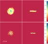 |
Fig. 1 Left: G1 run galaxy seen face-on. Right: G1 run galaxy seen edge-on. The upper panels show the distribution of the gas density (in log cm-3 units), and the bottom panels the distribution of stellar density for stars younger than 10 Myr (in arbitrary log units). |
2.2. Physics of galaxy formation
In this section, we briefly discuss how the physics (besides gravity and hydrodynamics) relevant to galaxy formation are modeled in the simulations. Table 2 summarizes the general properties of G1 and G2.
Comparison of the physical properties of G1 and G2.
Cooling: radiative energy losses, assuming gas is in collisional ionization equilibrium (CIE), are computed in each grid cell using the metallicity-dependent cooling functions tabulated in Sutherland & Dopita (1993). This allows the gas to cool down to 104 K in runs G1 and G2. In G2, we also account for the extra loss of energy provided by metal line cooling, following the prescription of Rosen & Bregman (1995). This allows the temperature of the gas to drop further, down to 100 K in this run.
Interstellar medium: to prevent numerical fragmentation, we assume the ideal gas transitions to a polytropic equation of state (EoS) in high-density regions  (1)where p is the polytropic index, ρ0 the gas density above which the polytropic law applies, and T0 the minimum temperature of the gas due to cooling. We adopt a p = 2 polytropic index that ensures that the Jeans length is independent of the gas density for densities above ρ0. For run G1, T0 = 104 K and ρ0 = 0.1 H cm-3, and the Jeans length of the gas is λJ ≃ 5.8 kpc, comparable to the size of the entire galactic disk. This means that the ISM gas does not fragment, but instead is smoothly distributed throughout the disk (see Fig. 1). For run G2, T0 = 100 K, and ρ0 = 10 H cm-3, so the constant Jeans length given by the polytropic EoS is λJ = 58 pc, which we resolve with around three cells of size Δx = 18 pc. This choice of T0 and ρ0 creates a multiphase medium with cold and dense bounded regions of size ~100 pc similar to the large giant molecular clouds (GMCs) of the Milky Way, and a low-density warm medium with strong turbulent motions (see Fig. 2).
Star formation: star formation is modeled as in Rasera & Teyssier (2006), with a random Poisson process spawning star cluster particles according to a classic Schmidt law. In other words, the star formation rate  scales with the local gas density ρ as
  (2)where tff is the free fall time and ϵ∗ is the star formation efficiency. We adopt ϵ∗ = 1% in runs G1 and G2, which is in fair agreement with observations over the gas density range we span (Krumholz & Tan 2007). Star formation is only permitted to occur in grid cells where the gas density is more than ρ0. Each star-cluster particle created is given a mass which is an integer multiple of the minimal mass m∗ = ρ0 × Δx3, where Δx is the size of a cell at the highest level of refinement. Therefore, our stellar mass resolution is m∗ ≃ 1.4 × 10³ M⊙ for the G2 simulation (and m∗ ≃ 7.7 × 10³ M⊙ for the G1 simulation). We forbid the star formation process to consume more than 90% of the gas mass in the cell where it takes place during a time step.
Feedback: we model supernovae (SN) feedback as in Dubois & Teyssier (2008); i.e., we deposit kinetic energy in a sphere centered on the explosion, along with mass and momentum distributed according to a Sedov-Taylor blast-wave profile. This kinetic approach ensures the formation of large-scale galactic winds in low-mass halos, and galactic fountains in the most massive ones even at low resolution (Dubois & Teyssier 2008). Such a precaution is necessary since it is well known that spurious thermal energy losses are catastrophic (Navarro & White 1993). We assume a standard Salpeter (1955) initial mass function (IMF), with ηSN = 10% (in mass) of the newly formed stars finishing their ~10 Myr lives as type II SN. We further assume that 1051 ergs of energy are released by each individual SN explosion with a typical ejected mass of 10 M⊙. Supernovae are also responsible for releasing metals into their surroundings with a constant yield y = 0.1. These metals are passively advected.
3. Lyα transfer
We use an improved version of the Monte Carlo radiation transfer code McLya of Verhamme et al. (2006) to post-process the two simulations G1 and G2 described in Sect. 2. The most notable technical improvement over the original McLya is that it now fully exploits the AMR grid structure of RAMSES, which allows us to perform the radiative transfer at the same spatial resolution than our hydrodynamics simulations. The new version of McLya also features more detailed physics of the Lyα line and UV continuum transfer, which include (see Schaerer et al. 2011): angular redistribution functions taking quantum mechanical effects for Lyα into account (Dijkstra & Loeb 2008; Stenflo 1980), frequency changes of Lyα photons from the recoil effect (e.g. Zheng & Miralda-Escudé 2002), the presence of deuterium (assuming a canonical abundance of D/H = 3 × 10⁻⁵, Dijkstra et al. 2006), and anisotropic dust scattering using the Henyey-Greenstein phase function (using parameters adopted in Witt & Gordon 2000).
Before McLya can be used to process our simulations, we have to extract a set of gas properties for each cell that are not directly predicted by RAMSES: the gas velocity dispersion due to temperature and small-scale turbulence (the macroscopic velocity and temperature of each cell are known), the ionization state (or equivalently the neutral hydrogen density), and the dust content. We discuss how we computed these quantities in the following sections, and then explain our strategy for sampling Lyα emission.
3.1. Ionization state of the gas
The simulation outputs provide us with the total density ρ of gas in each cell, including H, He, and metals. We derive the numerical density of H as nH = XHρ/mH, where XH = 0.76 is the mass fraction of H, and mH the mass of an H atom. Lyα photons, however, only scatter onto neutral hydrogen atoms (Hi), the numerical density of which we compute as nHI = x nH, where the neutral fraction x is evaluated assuming CIE, hence only depends on temperature T.
Using the polytropic equation of state (Eq. (1)) to prevent artificial fragmentation in the dense ISM unfortunately makes the gas temperature in these regions unknown. In all polytropic cells, we therefore set the temperature of the gas to T0 (=104 K in G1 and 102 K in G2). Since we are assuming CIE, these temperatures imply that all the polytropic gas is neutral.
3.2. Velocity dispersion of the gas
The transfer of Lyα photons through a parcel of gas depends on the velocity distribution of the neutral hydrogen atoms in that gas. This dependence appears in the Voigt profile through the Doppler parameter b. In the case of purely thermal motion, b = vth = (2kBT/mH)1/2. In the presence of small-scale turbulence, one has to quadratically add the turbulent velocity (vturb) contribution and write  .
.
In practice, we set vturb = 10 km s-1 in both G1 and G2 simulations. This value is the mean value of turbulent velocities computed in simulations of SN-driven turbulence by Dib et al. (2006). We tested the robustness of our results against this assumption by repeating the calculations presented in this paper with vturb = 0 or vturb = vth. We found no impact on the Lyα escape fractions.
3.3. Dust distribution
In our simulations, gas metallicity is self-consistently calculated from the release of metals in the ISM by SN explosion. The dust distribution is derived from the metallicity distribution by assuming a galactic value for the dust-to-metal (mass) ratio Rdust/metal = 0.3 (Inoue 2003). We further assume that dust is present only in neutral (i.e. T ≲ 104 K) media, and write  (3)where Z is the metallicity, mH/md = 5 × 10⁻⁸ the proton to dust particle mass ratio (Draine & Lee 1984), and nHI is the numerical density of neutral hydrogen derived in Sect. 3.1.
3.4. The Lyα sources
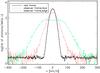 |
Fig. 3 Number of photons emitted per unit velocity bin. The black histogram shows the frequency distribution in the sources frame, as sampled by all photons used in our G2 experiment. This line profile is the one we use as a model for Hii regions (Sect. 3.4). The dotted red (resp. dashed blue) histograms show how these photons are distributed in the observer frame when the galaxy is seen face-on (resp. edge-on). |
In the present work, the only mechanism that produces Lyα photons and that we take into account is the recombination of photo-ionized gas surrounding massive stars (Kennicutt 1998). In practice, given our resolution, we are effectively using young star particles as a proxy for Hii regions and shooting photons from their locations. We only consider star particles younger than 10 Myr since they are the only ones producing significant amounts of ionizing photons (e.g. Charlot & Fall 1993).
Each one of these young star particles emits on average Nphot/N ⋆ photons1, where Nphot is the total number of photons in the experiment, and N ⋆ is the number of young stellar particles in the simulation. In our G1 simulation, we fix Nphot = 6.4 × 10⁵, and since this simulation has N⋆ ~ 103, this implies an average of 640 photons per source. In our G2 simulation, we pick Nphot ~ 5.1 × 10⁶, and since G2 contains N⋆ ~ 3 × 10⁴, this yields an average of 170 photons per source.
In the rest-frame of a star particle, the photons are emitted so as to sample a profile defined by a flat continuum plus a Gaussian line of full-width at half maximum of 20 km s-1, and of equivalent width EW(Lyα) = 200 Å (as suggested by, e.g., Charlot & Fall 1993; Valls-Gabaud 1993; Schaerer 2003). The continuum extends from −20 000 km s-1 to 20 000 km s-1 around the Lyα line in the star particle rest-frame, which is way beyond any resonant transfer effect. As an illustration, we show in Fig. 3 the source frame emission profile (black histogram) along with the emitted spectrum (emission from all star particles) of the face-on and edge-on G2 galaxy in the observer frame.
4. How the ISM structure affects Lyα transfer
The different temperature floors of the cooling functions used in G1 (104 K) and G2 (100 K) result in strikingly different structurations of the ISM. While the gas in G2 is able to fragment into small star-forming clumps, the thermal pressure support in G1 yields a rather smooth ISM with homogeneous star formation. In the present section, we investigate the influence of these structures on the Lyα escape fractions and line profiles.
4.1. Escape fractions
We first look at the escape fraction as a function of emission frequency fesc(vem), defined as the fraction of photons emitted at a frequency vem (in the source restframe) which eventually escape the galaxy (i.e. which are not absorbed by dust), whatever their observed frequency. The black curves in Fig. 4 show fesc as a function of vem for G1 (top panel) and G2 (bottom panel).
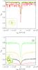 |
Fig. 4 Escape fraction as a function of emitted frequency vem (in the source restframe) for simulation G1 (top) and G2 (bottom). The black curves show the spatially integrated escape fractions, i.e. escape fractions averaged over all sources in the galaxy. The red (resp. yellow, green) curves show the escape fractions for sources in the high (resp. average, low) density regions. Thumbnails in the lower-left corner of each panel indicate the face-on position of sources contributing to each of the three curves of the same color. |
Before we discuss these curves in more detail, we can partially compare our results to those of Laursen et al. (2009). The simulations of these authors are relatively similar to our G1 simulation in the sense that their cooling curve also stops at 104 K (Sommer-Larsen et al. 2003) and therefore their ISM is unstructured on small-scales. As Laursen et al. (2009) only propagate Lyα photons emitted exactly at the Lyα frequency, we have to compare their escape fractions to our value at vem = 0, which is about 55%. This is broadly consistent with their results (their Fig. 9, at Mvir = 1010 M⊙).
We now turn to the comparison of the escape fractions predicted for G1 and G2 (black curves in Fig. 4). The first remarkable difference is seen in the continuum escape fractions2, which are ~95% in G1 versus ~22% in G2. This difference has a double origin. The first is the very different ISM structures found in G1 and G2. Since gas in G2 is able to cool to lower temperatures, it fragments into large starforming clouds within which most young stellar particles are buried. Instead, gas in G1 has stronger pressure support, star formation is more diffuse, and young stars end up being distributed in a rather low density environment. Indeed gas density in G1 does not reach values above ten atoms per cm3, while gas in G2 reaches 104 atoms per cm3. The second origin is that dust, which we model to scale with the density of metals (and neutral hydrogen) naturally follows star formation. Although it mixes on large scales with time, the dense star-forming clouds of G2 turn out to be more dust-rich than the diffuse (well mixed) ISM of G1. This produces more extinguished young stellar populations in G2, in agreement with e.g. Charlot & Fall (2000).
The second, more subtle point to take from Fig. 4 is that the escape fraction of Lyα photons is also less in G2 than in G1, even when normalized to that of the continuum. Indeed, the ratio of line center to continuum escape fractions in G1 and G2 are ~54% and ~20% respectively. We interpret this as a natural effect of resonant scattering of Lyα photons. In the dense clumps of G2 where most photons are emitted, the effect of dust is enhanced by the high Hi column densities that increase the path of photons, hence the likeliness of their hitting a dust grain. The Lyα escape fractions at the line center vary by an order of magnitude between our two simulated galaxies, from ~50% in G1 to ~5% in G2. Our simulations do not include ionizing radiation from the stellar sources (or from a UV background). This missing ingredient could increase the escape fractions, and possibly reduce the difference between G1 and G2. We plan to address this issue in a forthcoming paper.
Figure 4 also shows color histograms in each panel. These represent the escape fraction distributions for different populations of stars. The red (resp. yellow, green) curves show the escape fractions for photons emitted in high (resp. medium, low) density environments3. Thumbnail images in the lower lefthand corner of each panel show where the sources contributing to each curve are located in the galaxies (see Figs. 1 and 2 for comparison). The very strong variation of escape fractions with environment in G2, as opposed to the very small variation in G1, is the key to the difference between these two galaxies, and it explains our disagreement with the results of Laursen et al. (2009). This different behavior was expected, since the ISM in G1 (along with most simulations in the literature) is artificially smoothed on small-scales by the unrealistically high pressure support associated with 104 K gas. As a result, the weak radial variation in the escape fraction of G1 simply reflects the gas density gradient in that direction. In G2, however, most young stars lie within very dense and dusty clouds, as expected from, e.g., Charlot & Fall (2000), and consequently their Lyα radiation is heavily absorbed. These results demonstrate the necessity to resolve (at least some of) the ISM structure of galaxies with hydrodynamical simulations before postprocessing them with Lyα radiative transfer codes in order to make more realistic predictions for the Lyα escape fraction.
It may seem surprising that our results show the opposite trend as that expected in the scenario advocated by Neufeld (1991): we find that a clumpy ISM reduces the escape fraction of Lyα photons relatively to continuum photons instead of enhancing it. The reason for this behavior is that our G2 simulation predicts a configuration which is quite different from that assumed by Neufeld (1991). Whereas this author studies the propagation of photons through a clumpy medium, we find that our photons are actually mostly emitted within the clumps, and it is their (in)ability to escape from these clumps that dominates the results. Clearly, our G2 simulation still suffers from limitations, both in terms of the simplified assumptions we make to describe the ISM physics (no UV RT but CIE) and in terms of the resolution, which is insufficient for fully resolving Hii regions. Bearing these caveats in mind, we find no support for the “Neufeld scenario”. We plan to return to this issue with improved simulations in future work.
4.2. Lyα spectra
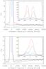 |
Fig. 5 Top: emergent spectra from G1 along 3 lines of sight (θ = 0 in magenta, θ = π/4 in green, θ = π/2 in blue). All spectra are spatially integrated, i.e. they are emergent spectra along a given direction, but from the whole galaxy. Bottom: same as top panel but for G2. |
We now turn to our predicted spectra, i.e. the distribution of observer-frame frequencies of photons that escape G1 and G2. We show these spectra in Fig. 5 for three different inclinations: face-on (magenta curves), edge-on (blue curves), and seen from 45 degrees (green curves). Thanks to the symmetry of the problem, we checked that the emergent spectra in all azimuthal directions are the same. The emergent spectra escaping at inclinations ± cosθ are also identical. To increase the statistics, we then sum all photons escaping with |cosθ| in the bin corresponding to the chosen inclination, regardless of its azimuthal angle φ. The spectra presented in Fig. 5 are built by collecting photons within cosθ bins large enough to a robust signal, but small enough to keep all the angular variations (e.g. |cosθ |> 0.95 face-on and |cosθ |< 0.05 edge-on). Our spectra are spatially integrated; i.e., they are emergent spectra along a given direction but from the whole galaxy.
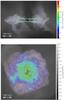 |
Fig. 6 Edge-on (top) and face-on (bottom) views of G1. In both panels, the gray scale indicates the density of neutral hydrogen (maximum value in a slice of thickness 8 high-resolution cells). The arrows indicate the velocity field of the gas at the location where photons last scatter before they are observed (the double sided arrow in the bottom left corner of each panel gives the scale), and their color scales with the log10 of the number of photons seen from each cell (red: lots of photons; blue: small number of photons). |
Looking at the spectra emerging from G1 in the top panel of Fig. 5, we see that they are all double-peaked, and roughly symmetrical about the line center. The overall intensity (and the equivalent width) decreases regularly from the face-on to the edge-on view. This is expected since the typical optical depth from the sources to the observer varies in the same way. The double-peaked symmetrical line resembles that expected from transfer through a static homogeneous medium. This is not surprising, since the ISM of G1 is rather homogeneous with a velocity field typical of a globally rotating disk with little internal motions (cf. Fig. 6, bottom panel). The somewhat higher intensity in the blue peak (at negative velocities) is the result of transfer effects through the gaseous halo, which is in part falling in towards the galaxy (cf. Fig. 6, top panel). Indeed, we checked that the spectrum of photons emerging face-on and for which the last scattering is in the halo (above the disk plane) is more asymmetric than that of photons emerging directly from the disk.
The emergent spectrum from G2 (bottom panel of Fig. 5) is also double-peaked edge-on, but clearly asymmetric face-on. The enhancement of the red peak compared to the blue peak is a signature of Lyα diffusing in an outflowing medium, and indeed, gas in G2 is flowing out at much higher velocities (a few 100 km s-1) than in G1 (where velocities are close to zero or infalling, see Figs. 6 and 7, top panels). We checked that if we set the velocity field to 0 km s-1 in each cell of the simulation, the spectrum of G2 seen in any direction becomes symmetric about the line center (v = 0 km s-1). We also reversed the vertical component of the velocity field, vz, and checked that in this case, the emergent spectrum is reversed, with a more prominent blue peak. Although a very strong large-scale galactic wind is present in G2, this outflowing material is mostly ionized and tenuous, conditions that render it transparent to Lyα photons. As can be seen from Fig. 2 (bottom left panel), SN feedback also pushes cold neutral gas outside the disk, albeit not very far. However, even such a small-scale kinematic feature is enough to produce the asymmetry observed in Fig. 5, because the kinematic energy transferred to this neutral gas is significant (cf. Fig. 7, top panel).
Even if the asymmetry of the G2 spectra qualitatively compares well to observations (e.g. Kulas et al. 2012, Fig. 10), the shift of the peak and the extension of the red tail are less important than in most observed spectra (e.g. Steidel et al. 2010, Fig. 1). We attribute (at least part of) this discrepancy to the mass of the galaxy we simulated. The latter is about two orders of magnitude less than typical Lyman-break galaxies, and therefore we can hardly expect its kinematics to have the same amplitude. A wrong implementation of the wind mechanism could cause the same mismatch. The simplified assumptions used to describe the ionization state of the interstellar gas, i.e. CIE, can also lead to an overestimate of the neutral fraction of the interstellar medium, especially in G2, and affect the spectral shapes. However, investigating different feedback recipes and following UV ionizing radiation transfer is beyond the scope of this paper.
5. Orientation effects
We discussed above the impact of the small-scale ISM structure on the propagation and escape of Lyα photons. In the present section, we inspect the global effect of inclination on the observed Lyα properties of our simulated galaxy G2. Indeed, orientation effects were predicted by Charlot & Fall (1993) and Chen & Neufeld (1994) and pointed out by recent studies (Laursen & Sommer-Larsen 2007; Laursen et al. 2009; Zheng et al. 2010; Barnes et al. 2011; Yajima et al. 2012b).
5.1. Angular escape fraction and angular redistribution
We begin by noting that the observed Lyα properties of G2 are, as expected, invariant around the axis of rotation of the disk, i.e. they do not depend on the azimuthal angle. They do, however, strongly depend on the inclination angle θ, which we define here as the angle from the rotation axis of the disk (θ = 0 face-on and θ = π/2 edge-on).
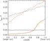 |
Fig. 8 Comparison between the distributions of escape directions in orange and emission directions in gray, for line (solid lines) and continuum (dashed lines) escaping photons. See the text for a detailed explanation of the shapes of these distributions. The y axis has two different meanings, fesc for the distribution of emission directions, and P for the normalized distribution of escape directions. |
The gray curves in Fig. 8 show the angular escape fractions of continuum (dashed line) and line (solid line) photons4. These escape fractions are computed as a function of the inclination at which photons are emitted. The flat solid gray line thus tells us that the escape fraction of line photons is isotropic: whatever direction they are emitted in, only about 5% will escape. In contrast, continuum photons tend to escape more easily when emitted perpendicular to the disk. Their escape fraction varies from 17% when emitted in the plane to 26% when emitted face-on. The difference between these behaviors is due to resonant scattering. Most line photons scatter a huge number of times (70% scatter more than 106 times, less than 10% scatter fewer than 10 times), enough to forget their initial direction. In contrast, continuum photons which escape do so without scattering (about 65% escape directly, and all escape with less than 8 scatterings).
The orange curves in Fig. 8 show the distributions of the inclinations with which the photons escape, i.e. the observed inclination angle distribution, again for continuum (dashed line) and line (solid line) photons. The solid orange curve of Fig. 8 shows a strong angular redistribution of line photons: although they are emitted isotropically and have an isotropic escape fraction, the probability (per unit solid angle) of one escaping face-on is about 15 times higher than that of one escaping edge-on. Similarly, albeit with a much lower amplitude, continuum photons are also redistributed in direction, so that they have a probability three times higher of coming out face-on than edge-on.
To understand this angular redistribution better, we show in Fig. 9 the relation between observed (y-axis) and emitted (x-axis) inclinations of the photons that escape. The top panel of Fig. 9 shows that, indeed, most continuum photons are observed with the same inclination as they were emitted with. This panel also shows that a small fraction of continuum photons emitted edge-on are scattered and observed as coming from any direction. The lower panel of Fig. 9 shows that the situation is quite different for line photons. Here, photons only have a marginal chance to escape in the same direction as they were emitted in, provided they were emitted almost face-on, and the overall redistribution is almost independent on the emission inclination. This is due, of course, to the very large number of scatterings that line photons undergo in general.
An early prediction of such orientation effect (favoring face-on escape) was made by Charlot & Fall (1993), by analogy with the stellar limb-darkening effect. However, the enhancement factor that we get (~15) is much higher than their prediction (~2.3).
This idealized simulation of galaxy formation may be a much more symmetrical configuration than galaxy formation in a cosmological context. However, if still relevant for real galaxies, the strong orientation effect we find has important observational implications. In particular, our results suggest that an LAE survey, which introduces a Lyα luminosity selection, will be biased towards face-on objects, and much more so than, e.g., Lyman break surveys that rely on a (UV continuum) broad-band selection. Hence the LAE may represent only an incomplete survey of star-forming objects at high redshifts. Also, we expect inclination to introduce a significant scatter in correlations between, e.g., SFR and observed Lyα luminosity.
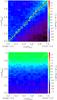 |
Fig. 9 Angular redistribution of continuum (top panel) and line (bottom panel) photons. The x-axis gives the emission direction (as the cosine of the inclination angle), and the y-axis gives the direction along which the photons escape. The color-coding scales logarithmically with the number of photon per unit area in the plot, as indicated by the color tables. The white lines on both panels, show the escape fraction as a function of the emission direction. |
5.2. Lyα equivalent widths
The inclination effect discussed above also manifests itself in the form of a strong correlation between the observed equivalent width and the inclination at which the galaxy is observed. In Fig. 10, we show the EW as a function of the inclination angle, each point corresponding to a random direction of observation. The tight correlation is well fit by a polynomial of the form EW(μ) = −8 + 80.7 μ − 393.1 μ2 + 798.2 μ3 − 387.4 μ4, where μ = cos(θ). This fit is shown with the solid black line. The scatter across the relation is due to variations in the azimuthal angle (φ). The EWs we compute here only take continuum radiation from stars younger than 10 Myr (the same that are used as sources for Lyα photons) into account, which is good approximation.
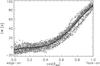 |
Fig. 10 Lyα equivalent widths as a function of the (cosine of the) inclination at which our simulated galaxy is seen. Each point marks one of 5000 mock observations. The solid line is a simple polynomial fit (see text). |
The strong dependency of the EW on μ illustrates the differential effect introduced by resonant scattering and discussed with Fig. 8. It shows the complexity of the possible bias introduced by EW selections in narrow-band5 LAE samples: not only does the Lyα luminosity of our simulated galaxy strongly vary with inclination, but the EW of its emission line does too, and as strongly. For example, with a typical selection at EW > 20 Å, our simulated galaxy would be found as an LAE only if observed with an inclination |μ| ≳ 0.6, i.e. with ~40% chance assuming a random inclination. In other words, if real galaxies behave like our simulation, LAE narrow-band surveys could be missing ~60% of the faint galaxy population at high redshifts. Even if this number is probably an upper limit, given the symetry of our idealized galaxy, it calls for observational studies that could assess the effect of inclination on the Lyα properties of real galaxies.
5.3. Line profile
As presented in Fig. 5, the emergent spectrum from our realistic ISM model G2 shows a transition in its shape with inclination: the edge-on profile is a double peak symmetrical around the line center, and the face-on spectrum has a very attenuated blue peak. The origin of this behavior is illustrated mainly in Fig. 7 and is as follows. Lyα photons seen escaping edge-on have scattered through an extremely thick medium, with low radial velocities, and the line they produce thus resembles the double peak of a static medium in which photons scatter until they are shifted far enough from the line center to escape. Lyα photons seen face-on, in contrast, traverse a much lower column density with a much more pronounced velocity field, with gas flowing out at velocities of several 100 km s-1, which favors the escape of red-shifted photons.
This evolution of the line profile suggests that the integrated spectral shapes of galaxies may reflect their inclination to some extent, as much as their internal structure and kinematics. Clearly, one would need a larger sample of simulated galaxies to draw robust conclusions here. However, this trend in our results does hint towards yet another selection effect: our simulation predicts a correlation between the EW and the line profile, thanks to the strong correlation that both these quantities have with inclination. This implies that an EW selection will favor asymmetric line profiles and tend to exclude double peaks, which we find to be associated to low inclinations.
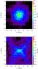 |
Fig. 11 Face-on (top) and edge-on (bottom) views of simulated galaxy G2 in Lyα. The color-coding shows surface brightness in arbitrary units, with the same scale in the two panels. |
6. Lyα halo
In Fig. 11, we present face-on (top panel) and edge-on (bottom panel) images6 of the galaxy G2 in the Lyα line. Scattering of Lyα photon through the tenuous intrahalo medium produces a diffuse Lyα halo that is clearly visible from both angles. The face-on view only includes photons with |cos(θ) |> 0.95. The edge-on view includes all photons with escaping |cos(θ) |< 0.2 so as to have enough statistics, and its surface brightness was renormalized accordingly, so that both panels in Fig. 11 are directly comparable. The observed Lyα luminosity face-on is 15% of the intrinsic luminosity (cf. Fig. 8, L(Lyα)obs = 0.15 × L(Lyα)int ~ 1.8 × 1041 erg s-1), whereas it is only a few percent in the edge-on sightline (~1–2 × 1040 erg s-1). Such a faint galaxy can be observed from z = 0 (Östlin et al. 2009, Lyman Alpha Reference Sample) until z ~ 3 (Rauch et al. 2008; Garel et al. 2012). As can be seen from the edge-on view, most of the extended emission comes from scattering on the envelope of the galactic wind produced by G2, and the hot wind itself is mostly transparent.
This picture is qualitatively comparable to observations by e.g. Hayes et al. (2005); Östlin et al. (2009) or Steidel et al. (2011). Quantitatively, we find that about 40% of Lyα photons come from the central region (within 1.5 kpc), and the rest is diffuse. This does not fit well with the results of Steidel et al. (2011), who find about five times more luminosity in the extended halo than in the central region. There are however a small number of likely explanations for this apparent disagreement. First, our simulated galaxy is about two orders of magnitude less massive than a typical LBG. Sect.nd, and probably more important, our simulation is idealized, and the circumgalactic medium does not feature cold streams or tidal tails, which would enhance the effect of scattering. Third, our calculations do not include in-situ emission from cold gas in the halo, either from cooling radiation or UV background fluorescence, and this may play a dominant role here (e.g. Rosdahl & Blaizot 2012).
7. Summary and conclusion
In this paper, we have studied the Lyα properties of a couple of high-resolution simulated dwarf galaxies forming in an idealized dark matter halo. Our two simulations assumed different temperature floors of the cooling function (104 K for G1, 100 K for G2), which result in strikingly different structurations of the ISM. While the gas in G2 is able to fragment into small star-forming clumps, the thermal pressure support in G1 yields a rather smooth ISM with homogeneous star formation. We have post-processed these galaxies with McLya in order to follow the resonant scattering of Lyα photons through their ISM and to predict their resulting observational properties. Our main results are as follows.
-
1.
As expected, the small-scale structure of the ISM plays adetermining role in shaping a galaxy’s Lyα properties. Inthe G2 simulation, where gas isallowed to cool down to temperatures ≪ 104 K, most young stars are embedded in thick, dusty, star-forming clouds, and the photons they emit are strongly attenuated. As opposed to the “Neufeld scenario”, the clumpiness of the ISM here enhances the destruction of Lyα photons relative to continuum photons, because photons are emitted within the dense clouds, à la Charlot & Fall (2000), rather than outside, as assumed in Neufeld (1991). In the G1 simulation, with an artificially warm ISM, young stars are found in much lower density environments and their photons escape more easily. This simulation is comparable to the previous studies in the literature that also include dust (Laursen et al. 2009; Yajima et al. 2012a,b), and our results are indeed similar to these studies. Such simulations do not capture the enhancement of Lyα extinction relative to continuum in star-forming regions that we find in G2, simply because they do not form such dense star-forming regions. Another important feature is the kinematic structure of the ISM. Because G2 develops a genuine multiphase medium, with very dense star-forming clouds and a tenuous diffuse component, supernovae explosions are able to push gas to high velocities (see Fig. 7). Instead, the rather homogeneous ISM of G1 is overall denser than the diffuse medium of G2, and resists supernovae explosions better. It thus displays a rather static velocity field (see Fig. 6). As shown in Sect. 4.2, these different velocity fields have a strong impact on the shape of Lyα lines.
-
2.
The analysis of Lyα emission from G27 demonstrates the existence of a strong inclination effect. Due to the numerous scatterings that line photons undergo, the probability of their escaping does not depend on the direction towards which they were emitted. Instead, they tend to systematically escape face-on, following the path of least opacity. Because continuum photons do not display such a strong angular redistribution, this effect is directly seen on the Lyα equivalent width, which we find to vary from ~− 5 Å edge-on to ~90 Å face-on. We also find that this inclination effect is seen in the shape of the Lyα line emerging from our simulated galaxy. When seen edge-on, our galaxy has a double-peak line, which is associated with a low EW. When seen face-on, our galaxy has an enhanced red peak and a high EW. These results suggest there are possibly strong observational biases in LAE surveys that necessarily rely on Lyα luminosity and EW selections and could thus tend to select face-on objects. As an example, a survey with an EW cut at 20 Å would select our galaxy only 40% of the time, assuming it has a random inclination.
-
3.
Scattering of galactic Lyα photons through the circumgalactic medium do produce an extended Lyα halo. We find that about a third of Lyα photons escaping G2 contribute to this diffuse component. This is somewhat at odds with the results of Steidel et al. (2011), though the comparison should be taken with caution given that our simulated galaxy has a much lower mass than the galaxies analyzed by these authors. Also, our simulation is idealized, and the CGM of G2 is not a good representation of what one finds in cosmological simulations at high redshift (Rosdahl & Blaizot 2012; Dubois et al. 2012).
Although our quantitative results are clearly limited by much that is missing in the physics, we believe that this work demonstrates the two main following points. (1) Resolving the ISM is mandatory if we want to understand the escape fraction of Lya from galaxies. It does not matter here if we have the correct solution: we show how widely the results vary when we change the ISM physics. And this definitely shows that we should go further). (2) For an ideal disk galaxy, we find that the escape fraction is a strong function of inclination, and we argue that this effect is quite possibly present in real galaxies (even though their morphologies are known to be more complex). Both results call for more work, both theoretically and observationally. From the theoretical viewpoint, we plan to make progress in forthcoming papers by (i) including the transfer of ionizing photons through a resolved ISM; and (ii) embedding our galaxy in the full complexity of its cosmological context.
The cuts in local stellar density that we used vary from G1 to G2, and are defined arbitrarily to capture the different regimes illustrated in Fig. 4.
We define line photons as having |vem| < 100 km s-1 in the frame of the sources (see black curve of Fig. 3). For continuum photons, we take photons with |vem| > 7000 km s-1.
Acknowledgments
A.V. was supported by a Fellowship for prospective researchers of the Swiss National Science Foundation to start this project in Oxford, and by a Marie Curie Intra European Fellowship within the 7th European Community Framework Program in Lyon. Y.D. is supported by an STFC Postdoctoral Fellowship. The simulations presented here were run on the TITANE cluster at the Centre de Calcul Recherche et Technologie of the CEA Saclay on allocated resources from the GENCI grant c2009046197. J.B. acknowledges support from the ANR BINGO project (ANR-08-BLAN-0316-01). We also acknowledge computing resources from the CC-IN2P3 Computing Center (Lyon/Villeurbanne – France), a partnership between CNRS/IN2P3 and CEA/DSM/Irfu.
References
- Barnes, L. A., Haehnelt, M. G., Tescari, E., & Viel, M. 2011, MNRAS, 416, 1723 [NASA ADS] [CrossRef] [Google Scholar]
- Bielby, R. M., Shanks, T., Weilbacher, P. M., et al. 2011, MNRAS, 414, 2 [NASA ADS] [CrossRef] [Google Scholar]
- Bullock, J. S., Dekel, A., Kolatt, T. S., et al. 2001, ApJ, 555, 240 [NASA ADS] [CrossRef] [Google Scholar]
- Cassata, P., Le Fèvre, O., Garilli, B., et al. 2011, A&A, 525, A143 [NASA ADS] [CrossRef] [EDP Sciences] [Google Scholar]
- Charlot, S., & Fall, S. M. 1993, ApJ, 415, 580 [NASA ADS] [CrossRef] [Google Scholar]
- Charlot, S., & Fall, S. M. 2000, ApJ, 539, 718 [NASA ADS] [CrossRef] [Google Scholar]
- Chen, W. L., & Neufeld, D. A. 1994, ApJ, 432, 567 [NASA ADS] [CrossRef] [Google Scholar]
- Dayal, P., Ferrara, A., & Gallerani, S. 2008, MNRAS, 389, 1683 [NASA ADS] [CrossRef] [Google Scholar]
- Dayal, P., Ferrara, A., Saro, A., et al. 2009, MNRAS, 400, 2000 [NASA ADS] [CrossRef] [Google Scholar]
- Dayal, P., Maselli, A., & Ferrara, A. 2011, MNRAS, 410, 830 [NASA ADS] [CrossRef] [Google Scholar]
- Dib, S., Bell, E., & Burkert, A. 2006, ApJ, 638, 797 [NASA ADS] [CrossRef] [Google Scholar]
- Dijkstra, M., & Loeb, A. 2008, MNRAS, 386, 492 [NASA ADS] [CrossRef] [Google Scholar]
- Dijkstra, M., Haiman, Z., & Spaans, M. 2006, ApJ, 649, 14 [NASA ADS] [CrossRef] [Google Scholar]
- Draine, B. T., & Lee, H. M. 1984, ApJ, 285, 89 [Google Scholar]
- Dubois, Y., & Teyssier, R. 2008, A&A, 477, 79 [NASA ADS] [CrossRef] [EDP Sciences] [Google Scholar]
- Dubois, Y., Pichon, C., Haehnelt, M., et al. 2012, MNRAS, 423, 3616 [NASA ADS] [CrossRef] [Google Scholar]
- Garel, T., Blaizot, J., Guiderdoni, B., et al. 2012, MNRAS, 422, 310 [NASA ADS] [CrossRef] [Google Scholar]
- Hayes, M., Östlin, G., Mas-Hesse, J. M., et al. 2005, A&A, 438, 71 [NASA ADS] [CrossRef] [EDP Sciences] [Google Scholar]
- Hu, E. M., Cowie, L. L., & McMahon, R. G. 1998, ApJ, 502, L99 [NASA ADS] [CrossRef] [Google Scholar]
- Hu, E. M., Cowie, L. L., Barger, A. J., et al. 2010, ApJ, 725, 394 [NASA ADS] [CrossRef] [Google Scholar]
- Inoue, A. K. 2003, PASJ, 55, 901 [NASA ADS] [CrossRef] [Google Scholar]
- Kennicutt, Jr., R. C. 1998, ApJ, 498, 541 [NASA ADS] [CrossRef] [Google Scholar]
- Komatsu, E., Smith, K. M., Dunkley, J., et al. 2011, ApJS, 192, 18 [NASA ADS] [CrossRef] [Google Scholar]
- Kravtsov, A. V., & Gnedin, O. Y. 2005, ApJ, 623, 650 [NASA ADS] [CrossRef] [Google Scholar]
- Krumholz, M. R., & Tan, J. C. 2007, ApJ, 654, 304 [NASA ADS] [CrossRef] [Google Scholar]
- Kudritzki, R.-P., Méndez, R. H., Feldmeier, J. J., et al. 2000, ApJ, 536, 19 [NASA ADS] [CrossRef] [Google Scholar]
- Kulas, K. R., Shapley, A. E., Kollmeier, J. A., et al. 2012, ApJ, 745, 33 [NASA ADS] [CrossRef] [Google Scholar]
- Laursen, P., & Sommer-Larsen, J. 2007, ApJ, 657, L69 [NASA ADS] [CrossRef] [Google Scholar]
- Laursen, P., Sommer-Larsen, J., & Andersen, A. C. 2009, ApJ, 704, 1640 [NASA ADS] [CrossRef] [Google Scholar]
- Le Delliou, M., Lacey, C. G., Baugh, C. M., & Morris, S. L. 2006, MNRAS, 365, 712 [NASA ADS] [CrossRef] [Google Scholar]
- Navarro, J. F., & White, S. D. M. 1993, MNRAS, 265, 271 [NASA ADS] [Google Scholar]
- Navarro, J. F., Frenk, C. S., & White, S. D. M. 1996, ApJ, 462, 563 [NASA ADS] [CrossRef] [Google Scholar]
- Neufeld, D. A. 1991, ApJ, 370, L85 [NASA ADS] [CrossRef] [Google Scholar]
- Orsi, A., Lacey, C. G., Baugh, C. M., & Infante, L. 2008, MNRAS, 391, 1589 [NASA ADS] [CrossRef] [Google Scholar]
- Orsi, A., Lacey, C. G., & Baugh, C. M. 2012, MNRAS, 425, 87 [NASA ADS] [CrossRef] [Google Scholar]
- Östlin, G., Hayes, M., Kunth, D., et al. 2009, AJ, 138, 923 [NASA ADS] [CrossRef] [Google Scholar]
- Ouchi, M., Shimasaku, K., Akiyama, M., et al. 2008, ApJS, 176, 301 [NASA ADS] [CrossRef] [Google Scholar]
- Ouchi, M., Shimasaku, K., Furusawa, H., et al. 2010, ApJ, 723, 869 [NASA ADS] [CrossRef] [Google Scholar]
- Rasera, Y., & Teyssier, R. 2006, A&A, 445, 1 [NASA ADS] [CrossRef] [EDP Sciences] [Google Scholar]
- Rauch, M., Haehnelt, M., Bunker, A., et al. 2008, ApJ, 681, 856 [NASA ADS] [CrossRef] [Google Scholar]
- Rosdahl, J., & Blaizot, J. 2012, MNRAS, 423, 344 [NASA ADS] [CrossRef] [Google Scholar]
- Rosen, A., & Bregman, J. N. 1995, ApJ, 440, 634 [NASA ADS] [CrossRef] [Google Scholar]
- Salpeter, E. E. 1955, ApJ, 121, 161 [Google Scholar]
- Schaerer, D. 2003, A&A, 397, 527 [NASA ADS] [CrossRef] [EDP Sciences] [Google Scholar]
- Schaerer, D., Hayes, M., Verhamme, A., & Teyssier, R. 2011, A&A, 531, A12 [NASA ADS] [CrossRef] [EDP Sciences] [Google Scholar]
- Shapley, A. E., Steidel, C. C., Pettini, M., & Adelberger, K. L. 2003, ApJ, 588, 65 [NASA ADS] [CrossRef] [Google Scholar]
- Shimasaku, K., Kashikawa, N., Doi, M., et al. 2006, PASJ, 58, 313 [NASA ADS] [Google Scholar]
- Sommer-Larsen, J. 2006, ApJ, 644, L1 [NASA ADS] [CrossRef] [Google Scholar]
- Sommer-Larsen, J., Götz, M., & Portinari, L. 2003, ApJ, 596, 47 [NASA ADS] [CrossRef] [Google Scholar]
- Steidel, C. C., Erb, D. K., Shapley, A. E., et al. 2010, ApJ, 717, 289 [NASA ADS] [CrossRef] [Google Scholar]
- Steidel, C. C., Bogosavljević, M., Shapley, A. E., et al. 2011, ApJ, 736, 160 [NASA ADS] [CrossRef] [Google Scholar]
- Stenflo, J. O. 1980, A&A, 84, 68 [NASA ADS] [Google Scholar]
- Sutherland, R. S., & Dopita, M. A. 1993, ApJS, 88, 253 [NASA ADS] [CrossRef] [Google Scholar]
- Tapken, C., Appenzeller, I., Noll, S., et al. 2007, A&A, 467, 63 [NASA ADS] [CrossRef] [EDP Sciences] [Google Scholar]
- Tasitsiomi, A. 2006, ApJ, 645, 792 [NASA ADS] [CrossRef] [Google Scholar]
- Tescari, E., Viel, M., Tornatore, L., & Borgani, S. 2009, MNRAS, 397, 411 [NASA ADS] [CrossRef] [Google Scholar]
- Teyssier, R. 2002, A&A, 385, 337 [NASA ADS] [CrossRef] [EDP Sciences] [Google Scholar]
- Truelove, J. K., Klein, R. I., McKee, C. F., et al. 1997, ApJ, 489, L179 [NASA ADS] [CrossRef] [Google Scholar]
- Valls-Gabaud, D. 1993, ApJ, 419, 7 [NASA ADS] [CrossRef] [Google Scholar]
- van Breukelen, C., Jarvis, M. J., & Venemans, B. P. 2005, MNRAS, 359, 895 [NASA ADS] [CrossRef] [Google Scholar]
- Verhamme, A., Schaerer, D., & Maselli, A. 2006, A&A, 460, 397 [NASA ADS] [CrossRef] [EDP Sciences] [Google Scholar]
- Witt, A. N., & Gordon, K. D. 2000, ApJ, 528, 799 [Google Scholar]
- Yajima, H., Li, Y., Zhu, Q., & Abel, T. 2012a, MNRAS, 424, 884 [NASA ADS] [CrossRef] [Google Scholar]
- Yajima, H., Li, Y., Zhu, Q., et al. 2012b, ApJ, 754, 118 [NASA ADS] [CrossRef] [Google Scholar]
- Zheng, Z., & Miralda-Escudé, J. 2002, ApJ, 578, 33 [NASA ADS] [CrossRef] [Google Scholar]
- Zheng, Z., Cen, R., Trac, H., & Miralda-Escudé, J. 2010, ApJ, 716, 574 [NASA ADS] [CrossRef] [Google Scholar]
All Tables
Comparison of the four published studies of Lyα radiation transfer through the interstellar medium of galaxies with this study.
All Figures
|
Fig. 1 Left: G1 run galaxy seen face-on. Right: G1 run galaxy seen edge-on. The upper panels show the distribution of the gas density (in log cm-3 units), and the bottom panels the distribution of stellar density for stars younger than 10 Myr (in arbitrary log units). |
| In the text | |
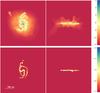 |
Fig. 2 Same as Fig. 1 for the G2 run. |
| In the text | |
|
Fig. 3 Number of photons emitted per unit velocity bin. The black histogram shows the frequency distribution in the sources frame, as sampled by all photons used in our G2 experiment. This line profile is the one we use as a model for Hii regions (Sect. 3.4). The dotted red (resp. dashed blue) histograms show how these photons are distributed in the observer frame when the galaxy is seen face-on (resp. edge-on). |
| In the text | |
|
Fig. 4 Escape fraction as a function of emitted frequency vem (in the source restframe) for simulation G1 (top) and G2 (bottom). The black curves show the spatially integrated escape fractions, i.e. escape fractions averaged over all sources in the galaxy. The red (resp. yellow, green) curves show the escape fractions for sources in the high (resp. average, low) density regions. Thumbnails in the lower-left corner of each panel indicate the face-on position of sources contributing to each of the three curves of the same color. |
| In the text | |
|
Fig. 5 Top: emergent spectra from G1 along 3 lines of sight (θ = 0 in magenta, θ = π/4 in green, θ = π/2 in blue). All spectra are spatially integrated, i.e. they are emergent spectra along a given direction, but from the whole galaxy. Bottom: same as top panel but for G2. |
| In the text | |
|
Fig. 6 Edge-on (top) and face-on (bottom) views of G1. In both panels, the gray scale indicates the density of neutral hydrogen (maximum value in a slice of thickness 8 high-resolution cells). The arrows indicate the velocity field of the gas at the location where photons last scatter before they are observed (the double sided arrow in the bottom left corner of each panel gives the scale), and their color scales with the log10 of the number of photons seen from each cell (red: lots of photons; blue: small number of photons). |
| In the text | |
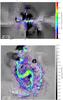 |
Fig. 7 Same as Fig. 6, for G2. Note the much more pronounced vertical motions in the top panel. |
| In the text | |
|
Fig. 8 Comparison between the distributions of escape directions in orange and emission directions in gray, for line (solid lines) and continuum (dashed lines) escaping photons. See the text for a detailed explanation of the shapes of these distributions. The y axis has two different meanings, fesc for the distribution of emission directions, and P for the normalized distribution of escape directions. |
| In the text | |
|
Fig. 9 Angular redistribution of continuum (top panel) and line (bottom panel) photons. The x-axis gives the emission direction (as the cosine of the inclination angle), and the y-axis gives the direction along which the photons escape. The color-coding scales logarithmically with the number of photon per unit area in the plot, as indicated by the color tables. The white lines on both panels, show the escape fraction as a function of the emission direction. |
| In the text | |
|
Fig. 10 Lyα equivalent widths as a function of the (cosine of the) inclination at which our simulated galaxy is seen. Each point marks one of 5000 mock observations. The solid line is a simple polynomial fit (see text). |
| In the text | |
|
Fig. 11 Face-on (top) and edge-on (bottom) views of simulated galaxy G2 in Lyα. The color-coding shows surface brightness in arbitrary units, with the same scale in the two panels. |
| In the text | |
Current usage metrics show cumulative count of Article Views (full-text article views including HTML views, PDF and ePub downloads, according to the available data) and Abstracts Views on Vision4Press platform.
Data correspond to usage on the plateform after 2015. The current usage metrics is available 48-96 hours after online publication and is updated daily on week days.
Initial download of the metrics may take a while.