| Issue |
A&A
Volume 546, October 2012
|
|
|---|---|---|
| Article Number | A102 | |
| Number of page(s) | 12 | |
| Section | Planets and planetary systems | |
| DOI | https://doi.org/10.1051/0004-6361/201118451 | |
| Published online | 12 October 2012 | |
Wind mapping in Venus’ upper mesosphere with the IRAM-Plateau de Bure interferometer
1
National Radio Astronomy Observatory, Charlottesville
VA-22902,
USA
e-mail: This email address is being protected from spambots. You need JavaScript enabled to view it.
2
Harvard-Smithsonian Center for Astrophysics,
Cambridge
MA-02138,
USA
3
LESIA-Observatoire de Paris, 5 place J. Janssen, 92195
Meudon Cedex,
France
4
National Institute of Information and Communications
Technology, 4-2-1 Nukui-kita,
Koganei, Tokyo,
Japan
Received: 14 November 2011
Accepted: 16 February 2012
Abstract
Context. The dynamics of the upper mesosphere of Venus (~85–115 km) have been characterized as a combination of a retrograde superrotating zonal wind (RSZ) with a sub-solar-to-antisolar flow (SSAS). Numerous mm-wave single-dish observations have been obtained and been able to directly measure the mesospheric line-of-sight winds by mapping the Doppler shifts of CO rotational lines, but their limited spatial resolution makes their interpretation difficult.
Aims. By using interferometric facilities, one can achieve a higher resolution in Doppler-shift maps, allowing us in particular to place firmer constraints on the respective contributions of the SSAS and RSZ circulations to the global mesospheric wind field.
Methods. We report on interferometric observations of the CO(1-0) line obtained with the IRAM-Plateau de Bure interferometer in November 2007 and June 2009, which was able to map the upper mesosphere dynamics on the morning hemisphere with a high spatial resolution (3.5–5.5′′).
Results. All the obtained measurements show, with a remarkably high temporal stability, that the wind globally flows in the (sky) east-west direction, corresponding in the observed geometry to either an unexpected prograde zonal wind or a SSAS flow. A very localized inversion of the wind direction, which could correspond to a RSZ wind, is also repeatedly detected in the night hemisphere. The presence of significant meridional winds is not evidenced. Using models with different combinations of zonal and SSAS winds, we find that the data is most accurately reproduced by a dominant SSAS flow with a maximal velocity at the terminator of ~200 m/s, displaying large diurnal and latitudinal asymmetries, combined with an equatorial RSZ wind of 70–100 m/s. Overall, this is indicative of a wind-field structure consistent with but much more complex than the usual representation of the mesospheric dynamics.
Key words: planets and satellites: atmospheres / planets and satellites: individual: Venus / instrumentation: interferometers
© ESO, 2012
1. Introduction
The bulk of Venus’ atmosphere is usually described as the superposition of three different regions presenting significantly different thermal structures and dynamical regimes. The troposphere is the deepest region and extends up to the top of the cloud deck (~65 km altitude). This region displays a global strong retrograde superrotating zonal wind (RSZ), whose centrifugal force is believed to balance the latitudinal temperature gradient, thus maintaining a planet-wide cyclostrophic equilibrium. The Pioneer and Venera probes revealed that there is a significant increase in the wind velocity with altitude in the troposphere, equatorial velocities Veq of up to ~100 m/s being reached in the cloud deck (Gierasch et al. 1997), a result that has been confirmed by the tracking of ultraviolet cloud features performed by Mariner, Pioneer, and Galileo spacecrafts (see review in Limaye 2007) and, later, the VMC monitoring camera and VIRTIS imaging spectrometer on board Venus Express (Markiewicz et al. 2007; Sánchez-Lavega et al. 2008).
Above 115 km lies the thermosphere, where the temperature distribution is mainly controlled by the solar EUV heating. As a consequence, the very steep temperature gradient between the night and day hemispheres (up to 150 K, see Kasprzak et al. 1997) should drive a strong sub-solar to anti-solar (SSAS) wind. Models of the thermospheric SSAS wind (Bougher et al. 1986) have predicted that the flow should be symmetric around the sub-solar/anti-solar line, and that its velocity should increase almost linearly with the solar incidence angle, to reach a maximum velocity Vter near the terminator of up to 230 m/s above 150 km. The possibility of a SSAS wind in the thermosphere is supported by the spatial distribution of light species and NO airglows, which are concentrated at post-midnight local times (Bougher et al. 1997; Gérard et al. 2008) and indicative of the coexistence of an highly temporally variable RSZ wind. The main mechanism invoked to maintain the RSZ wind in the thermosphere is the breaking of gravity waves generated in the cloud deck (Bougher et al. 1997).
Observational parameters of Venus at the observation dates.
In-between these layers lies the mesosphere (65–115 km). Dynamically, this region is viewed as a transition zone, where both SSAS and RSZ winds coexist, as confirmed by numerous observations. At the lower boundary of the mesosphere, corresponding to the top of the cloud deck (~68 km), the winds’ line-of-sight projection can be directly measured from the Doppler shifts of the reflected solar Fraunhofer lines on the day-side. Examples of these observations by Widemann et al. (2007, 2008) revealed a strong and dominant RSZ wind with Veq ~ 100 m/s and possibly meridional winds (on the order of 10 m/s), as well as large temporal variations, although the latter are not seen in cloud tracking observations sounding just a few kilometers below (Moissl et al. 2009).
Between 85 km and 110 km (upper mesosphere), Doppler-shift measurements can be obtained from mm-wave CO rotational lines or infrared (IR) CO2 emission lines outside local thermal equilibrium observed by heterodyne spectroscopy. Most results have been interpreted as a combination of SSAS and RSZ winds (see e.g. Lellouch et al. 1994; Clancy et al. 2008; Lellouch et al. 2008; Sornig et al. 2008), with variable relative contributions: Vter is usually inferred to be on the order of 100 m/s, while Veq varies between 0 and 200 m/s, and may not be sufficient to maintain cyclostrophic equilibrium (Piccialli et al. 2008; Piccialli 2010). Poleward meridional winds may also have been marginally detected (Lellouch et al. 1994, 2008). In addition to large temporal variations over timescales as short as a few hours (Clancy et al. 2011), modifications of the SSAS and RSZ wind-fields with latitude (Sornig et al. 2008; Lellouch et al. 2008), as well as variations in the wind velocity with altitude (Lellouch et al. 2008; Clancy et al. 2011) have also been observed. Prograde zonal winds were also recently suggested based on some day-side measurements of the CO(2–1) line by Lellouch et al. (2008). The possible driving mechanism for a prograde zonal wind is unknown. Furthermore, based on an analysis of a large number of night-side observations, Clancy et al. (2011) suggested the existence of large-scale circulations, that cannot be explained by a combination of RSZ and SSAS winds.
The interpretation of Doppler shifts in terms of wind field is complex owing to the difficulty in distinguishing between he RSZ and SSAS winds depending on the observing geometry and, for mm-wave observations, the lack of spatial resolution available using single-dish facilities. In the 95–115 km altitude region, an indirect way of characterizing winds consists in mapping O2, NO, and OH airglows (see e.g. Gérard et al. 2008). As in the thermosphere, their post-midnight concentration indicates the dominance of the SSAS wind with respect to the RSZ wind. Using the VIRTIS imaging spectrometer on board the European Venus Express spacecraft, Hueso et al. (2008) were able to track O2 airglows confirming the dominant SSAS wind, but also displaying additional features interpreted as highly spatially variable retrograde zonal and meridional winds, as well as prograde zonal winds.
More recently Hueso et al. (2008); Lellouch et al. (2008) and Clancy et al. (2011) accumulated evidence of spatial and temporal variations in the upper mesosphere wind field, hence supporting a more complicated picture of the mesospheric circulation than a simple combination of SSAS and RSZ winds.
One key factor in improving the knowledge and understanding of the upper mesosphere dynamics is to increase the spatial resolution when mapping mm-wave Doppler shifts. Currently available single-dish facilities can offer at best a resolution of 8′′ at 345 GHz and 21′′ at 115 GHz (with the IRAM-30 m telescope), while Venus’ disk size varies between 8′′ and 58′′. In addition to smoothing out the information over relatively large spatial scales, single-dish observations typically require multiple pointings to reconstruct the wind field across Venus’ disk, at the expense of integration time per pointing. The interferometric mapping of Doppler shifts performed by antenna arrays provides higher spatial resolution data than single-dish observations, which is especially necessary to map the disk at maximal elongations and superior conjunction geometries, during which the day-side of Venus is observable. A resolution better than 3′′ was for example reached in the only previously published Venus’ interferometric Doppler-shift maps (Shah et al. 1991), obtained at the Owens Valley Radio Observatory (OVRO) array.
This paper presents interferometric observations of the CO(1–0) (115 GHz) rotational line obtained at the Institut de Radio-Astronomie Millimétrique Plateau de Bure Interferometer (IRAM-PdBI) in November 2007 and June 2009, in two consecutive days in each of these months. All observations were performed near the maximum western elongation of Venus, mapping the morning hemisphere with a spatial resolution of between 3.5′′ and 5.5′′. We present our Doppler-shift maps and their possible interpretation in terms of wind field using different combinations of SSAS and zonal winds, along with the determination of the sounded altitudes, to provide the most possible complete snapshot view of the upper mesosphere dynamics on Venus.
2. Observations
2.1. November 2007
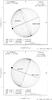 |
Fig. 1 Aspect of Venus on November 16, 2007 (top) and June 12, 2009 (bottom). The black dot next to the eastern limb represents the sub-solar point. The small circle at the center represents the sub-earth point. Coordinates of the sub-earth and sub-solar points are indicated in the east longitude convention, along with the pole axis tilt angle. From http://www.imcce.fr |
The first set of observations was performed on 16 and 17 November 2007, with the IRAM-Plateau de Bure Interferometer, located in the southern French Alps. Observational parameters and ephemeris are gathered in Table 1. At the time, Venus was close to its maximum western elongation, corresponding to the morning hemisphere view, such that both the day-side and the night-side could be observed (see Fig. 1, top panel). This geometry is the most appropriate to directly measure the zonal wind contribution near the limbs, where, according to the Bougher et al. (1986) model, the contribution of SSAS wind should be minimal.
The array, with five operating antennas of 15 m diameter each, was in the C configuration with maximum baseline length (distance between antennae projected in a plane perpendicular to the line-of-sight) of 180 m in the east-west direction. The obtained coverage of the Fourier plane, as determined from the relative positions of the antennae and the track of the source in the sky, is represented in Fig. 2 (top-right panel). The Fourier-plane filling appears to be very poor, especially in what corresponds to the north-south direction in the image plane, owing to the low declination of Venus at the time of the observations (~1°).
After merging the two datasets, the synthesized beam obtained, which corresponds to the spatial resolution of the final map, is a very elongated ellipse with a half-power beam width (HPBW) of ~5 × 2′′ at 115 GHz. Figure 2 (top-left panel) shows the amplitude of the obtained data (i.e., complex visibilities in the Fourier plane) as a function of the projected baseline length. The observed shape roughly corresponds to the Fourier transform of a disk and the multiple nulls illustrate the high spatial resolution achieved. The primary beam of the antennae (44.5′′) is so large that it cannot resolve Venus’ disk (~20′′ diameter). Nonetheless, this convolution by the primary beam is taken into account in the models presented in the following sections.
The CO(1–0) line at 115.271 GHz was observed in the upper sideband (USB) of the tuned receivers in a 20 MHz-wide spectral window with a 39 kHz spectral resolution (corresponding to a velocity resolution of 101 m/s at 115 GHz), while the continuum was simultaneously integrated on three spectral windows totalling 940 MHz of bandwidth. The data were measured simultaneously using two cross-polarized receivers that, assuming the source emission is unpolarized, can be assumed to be equivalent but independent, thus effectively doubling the amount of collected data with respect to a single-receiver system.
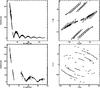 |
Fig. 2 Continuum visibilities obtained in November 2007 (top panels, merged data from the two observing dates) and June 2009 (bottom panels, data from June 13). Left panels: amplitude (in Jy) of the visibilities, plotted against projected baseline length (in meters). Right panels: corresponding Fourier-plane coverage. The units correspond to the component of the projected baselines in the east-west (U) and north-south (V) directions (in m). |
The calibration of the obtained raw data (visibilities) was performed with the GILDAS-CLIC data reduction package developed at IRAM1. Temporal gain calibration of the phase and amplitude of the visibilities was achieved by using as a point-source reference the quasar 1055+018, which was observed every 35 min. The atmospheric phase calibration provided by the 22 GHz water vapor radiometers was also applied. The spectral bandpass response was determined using the quasars 3c454.3 and 3c273, allowing correction down to the 0.5% level.
To increase the quality of the high spectral resolution data (CO line data), assuming that the continuum distribution is known to a high precision level, we were able to self-calibrate the data phase using a continuum model (see Sect. 3.1 for details). The calibrated visibilities were then imaged by applying both an inverse fast Fourier transform and deconvolution of the secondary lobes. This was particularly difficult to achieve because of the incompleteness of the Fourier-plane filling. Our most robust results were obtained by combining the two datasets (accounting for the change in the apparent size of Venus by accordingly changing the Fourier-plane scale) and tapering the visibilities, i.e., decreasing the contribution from the longest baselines. After deconvolution using the HOGBOM method (Högbom 1974), the synthesized beam size was 5.7 × 3.6′′.
The final output of these observations consists of interferometric maps of the continuum emission, and of interferometric maps of the CO(1–0) line (datacubes) obtained from the high spectral resolution window. The noise rms of ~0.7 Jy/beam on each 39 kHz-wide spectral channel is mainly determined by the imaging dynamic range, and corresponds to a signal-to-noise ratio (S/R) of 100 per beam at most.
2.2. June 2009
During the June 2009 observations, Venus was in a similar observing geometry as in 2007 (morning hemisphere view, see Fig. 1, bottom panel).
The array was this time in the D configuration (with maximum projected baseline length of 95 m), and the half-power beam width at 115 GHz was 4.1 × 4.1′′ on June 12 and 5.7 × 3.4′′ on June 13, allowing us to resolve Venus’ disk (~22′′ diameter) in up to six independent points across.
The same spectral setup as in 2007 was used to target the CO(1–0) line. The phase and amplitude temporal gain calibration was performed in the same manner as in 2007, using the quasars 0119+115 and 0235+164 as gain calibrators, and the strong quasar 3c454.3 for bandpass calibration down to a 1% level.
Thanks to a much better Fourier-plane filling than in 2007 (see Fig. 2, bottom-right panel), the imaging, performed using the SDI deconvolution method (Steer et al. 1984), was much more satisfactory. The June 13 data was eventually tapered, so as to obtain a synthesized beam degraded to a HPBW of 5.7 × 5.3′′, ensuring a higher S/R per beam.
The final noise rms reached in the interferometric map is approximately 0.2 Jy/beam in each 39 kHz-wide spectral channel on June 12 (resp. 0.5 Jy/beam on June 13), still mainly limited by the imaging dynamic range. This corresponds to a S/R in the map of 350 per beam at most (resp. 230).
3. Data analysis
3.1. Continuum-based phase self-calibration
To obtain satisfactory imaging quality, we choose to self-calibrate the phase of the obtained data visibilities, i.e. to force the continuum data phase to follow a model. This procedure is commonly performed for interferometric datasets (see e.g. Moullet et al. 2008; Moreno et al. 2009), and can significantly improve the phase calibration, provided that the continuum brightness distribution is well-known a priori.
On Venus, the continuum emission at 115 GHz corresponds to the CO2-CO2 collision-induced pseudo-continuum formed in the cloud deck around 1 bar (40–50 km altitude, see e.g. Gurwell et al. 1995). To model this emission, we use a radiative transfer code adapted from Lellouch et al. (1994), assuming standard temperature/pressure profiles, and accounting for curvature at the limb. Minor species SO2 and H2SO4, which produce additional opacity around 115 GHz, are included in the models with a typical content of 130 ppm SO2 and 5 ppm H2SO4 at 40 km. Although some observers have suggested that spatial variations in the continuum level of up to 10% may be present (de Pater et al. 1991), possibly owing to the distribution of absorbers or strong horizontal temperature gradients, we assume that the continuum-emission spatial distribution corresponds to a limb-darkened disk, owing to the smooth variation with airmass in the CO2-CO2 opacity. The continuum model produced by our radiative transfer code is used as the reference model for phase self-calibration. The corresponding visibilities phases are computed using the same Fourier-plane coverage as the data. Once corrections from the continuum data to the model are derived for each antenna pair (baseline), they are applied to the phase of the CO line data. We note that the choice of absorber content, within a reasonable range, does slightly change the limb-darkening profile of the model, but has very little influence on the result of the self-calibration.
The assumed continuum model produces a disk-averaged brightness temperature of 330 K at 115 GHz, which is used as the reference to assess the absolute flux scale of the data.
3.2. CO line maps
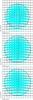 |
Fig. 3 Maps of Venus’ CO(1–0) spectra (in Jy/beam), for different observing dates. The location of each spectrum with respect to the disk center is indicated in parenthesis (in arcseconds). The velocity scale for each individual spectrum goes from −2 to + 2 km s-1. The continuum level is represented by the blue background. In each panel, Venus’ disk is represented by the centered circle, the synthesized beam by the ellipse in the bottom left hand corner, and the terminator by the vertical arc. The maps were rotated so that the pole axis is vertical in the figure. Top panel: 2007 observations (merged data from the two observing dates). The flux scale goes from 0 to 75 Jy/beam. Middle panel: June 12, 2009 observations. The flux scale goes from 0 to 75 Jy/beam. Bottom panel: June 13, 2009 observations. The flux scale goes from 0 to 120 Jy/beam. |
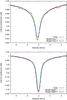 |
Fig. 4 CO(1–0) lines measured on June 12, 2009, plotted against synthetic lines computed assuming adjusted atmospheric models. Model 1 (for day and night conditions) corresponds to a model where only the temperature profile is adjusted, while the CO mixing profile is fixed to the reference profile. Model 2 (for day and night conditions) corresponds to a model where only the CO mixing profile is adjusted, while the temperature profile is fixed to the reference profile. Top: day-side spectra measured on the equator at 8′′ from the sub-earth point (9.3 am local time). Bottom: night-side spectra measured on the equator at 8′′ from the sub-earth point (3.1 am local time). |
The CO(1–0) line datacubes are represented in Fig. 3 as maps of spectra sampled on a grid with 2′′ resolution, where each spectrum corresponds to the local, beam-convolved spectrum. These maps illustrate the final imaging quality that can be achieved. All maps display absorption lines all over the disk, with the expected characteristic profile, i.e. Lorentzian-shaped broad wings and a Doppler-broadened core of ~1 km s-1 width. One day-side line and one night-side line are plotted with an expanded scale in Fig. 4, showing the excellent quality of the individual spectra obtained in 2009.
Since, within the CO line, the brightness temperature at a given frequency is controlled by the atmospheric structure (temperature and CO mixing ratio vertical profiles, and the airmass at Venus) in the sounded atmospheric levels, a qualitative assessment of the variation in the CO(1–0) line-to-continuum ratio across Venus’ disk can give an indication of the horizontal distribution of temperature and/or CO mixing ratio in the upper mesosphere.
Previous mm-wave observations indicate deeper CO line absorptions on the night-side than on the day-side (see e.g. Clancy & Muhleman 1985). The present observations qualitatively confirm these findings. In 2007, the line-to-continuum ratio at the equator varied from 11% to 48% from the sky-east (noon) to sky-west limb (midnight), with a maximum depth near 1 am local time. In 2009, the ratio varied from 19% to 47% on June 12, (respectively 12% to 47% on June 13), and the maximum depth was measured near 3 am local time. The variation in the CO line depth has been interpreted as the signature of a steeper thermal gradient on the night-side compared to the day side and/or a higher mixing ratio of CO (Clancy & Muhleman 1985, by a factor up to four), resulting from a strong SSAS wind displacing the CO away from the day-side (where it is produced by CO2 photolysis). With only one line available in our dataset, we cannot distinguish between the two hypotheses.
3.3. Doppler-shift maps
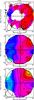 |
Fig. 5 Maps of the Doppler shifts (in m/s) measured in the core of the CO(1–0) lines, for different observing dates. Regions where Doppler shifts could not be retrieved appear as blank. In each panel, Venus’ disk is represented by the centered circle, the synthesized beam by the ellipse in the bottom left-hand corner, and the terminator by the vertical arc. The contour step corresponds to 20 m/s. The maps were rotated to ensure that the pole axis is vertical in the figure. Top panel: 2007 observations (merged data from the two observing dates). Doppler-shift errors are on the order of 25–35 m/s on the day-side and 15–20 m/s on the night-side. Middle panel: June 12, 2009 observations. Errors are on the order of 10 m/s on the day-side and 6 m/s on the night-side. Bottom panel: June 13, 2009 observations. Errors are on the order of 15–22 m/s on the day-side and 7 m/s on the night-side. |
Measurements of the Doppler shifts of the CO lines (i.e. offsets from the CO(1–0) line rest frequency) were performed across the spectral maps. Specifically, the data cubes were sampled on a spatial grid with one arcsecond wide cells, and each spectrum from each cell was analyzed, using the GILDAS-CLASS line analysis package. To take into account only the inner Doppler-broadened line core in the fit, the outer Lorentzian profile was fitted by a seventh order polynomial. The fitted spectral baseline was then removed from the full spectrum, so as to extract only the core (± 0.5 km s-1). This procedure affected neither the shape of the line core nor its Doppler shift. The obtained line core was finally fit by a Gaussian profile. Even if the line core does not have a perfectly Gaussian profile, if its profile is symmetric, the results for the central frequency fit are insensitive to the fitting profile. Only Gaussian fits performed on lines detected with a confidence higher than 5σ were considered for the analysis. The Doppler-shift maps obtained by this technique are represented in Fig. 5.
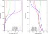 |
Fig. 6 Atmospheric models adjusted to the CO(1–0) lines represented in Fig. 4. Left: CO mixing ratio profiles. Right: temperature profiles. |
In the 2007 data (Fig. 5, top panel), owing to the very low quality of the data imaging, even after merging the datasets from the two consecutively observed days Doppler shifts cannot be measured over a significant fraction of the disk. In particular, in regions where the CO lines are very shallow and the imaging quality is as its worst, CO lines could not be detected with sufficiently high confidence. The uncertainties in each measurement are also very high. Globally, we note that blue-shifts (corresponding to approaching winds) are dominant on the day-side, with values of 50 m/s at most and measurement errors on the order of 25–35 m/s. On the night-side measurement errors are lower (15–20 m/s), and mostly red-shifts (corresponding to receding winds) are measured with values up to 50 m/s. At southern latitudes near the western limb (~1 am local time), the Doppler shifts display a sign inversion, with blue shifts values of −30 m/s ± 15 m/s. Analyzing separately the data of the two observed days, even fewer Doppler-shift measurements can be performed, but the Doppler-shift pattern derived is globally the same, suggesting the stability of the wind large scale characteristics over the 24 h span between the observations, and altogether arguing in favor of the reality of the global wind pattern observed. However, the relatively low significance (2–3σ) of the individual Doppler shifts obtained does not justify further analysis or accurate modeling of the 2007 data.
On the 2009 data (Fig. 5, middle and bottom panels), the uncertainties obtained are much lower, on the order of 10 m/s on June 12 on the day-side (resp. 15–22 m/s on June 13), and of 6 m/s on the night-side (resp. 7 m/s). A more detailed analysis of the Doppler-shift maps can then be performed.
We observe that the Doppler-shift maps acquired during the two consecutive days in 2009 have a very similar pattern, with little variations in the measured values, characterized by:
-
blue-shifts on the day-side, with velocities up to70 m/s on June 12 (resp. 90 m/s onJune 13).
-
red-shifts on the night-side with velocities up to 60 m/s on June 12 (resp. 100 m/s on June 13), and significant variations with latitude.
-
blue-shifts in a small region located on the night-side near the equator and at low southern latitudes, hereafter referred to as the blue-night (BN) region, with values up to −50 m/s on June 12 (resp. −30 m/s on June 13).
We also note that the pattern observed in 2009 globally corresponds to the pattern tentatively observed in 2007, although the similarity is difficult to assess quantitatively.
The measured Doppler shifts correspond to beam-convolved velocities projected along the line-of-sight (LOS), and differ from the actual atmospheric wind velocities by a projection factor depending on the position on the disk, the flow direction, and the beam profile. Therefore a wind field cannot directly be proposed based on the LOS winds but requires deconvolution of the various components.
3.4. Estimation of probed altitude
To give a sense of the atmospheric region that is sounded by the CO(1–0) line, we performed an approximate modeling of the line emission. The contribution of each atmospheric level is determined by the opacity function of the line, which can be calculated using a radiative transfer model and assuming the atmospheric temperature and CO mixing ratio profiles. When multiple transitions with different opacities are available, it is possible to independently retrieve the temperature and CO mixing ratio profiles by performing a simultaneous fitting of the line shapes (see e.g. Clancy et al. 2008), and in turn calculating the contribution from each altitude. However, it is impossible to assess unequivocally the temperature and mixing ratio profiles from a single transition dataset. In our case, since we did not know a priori the appropriate temperature and CO mixing ratio profiles, we used an alternative, approximate approach, by considering, for both day and night conditions, two very different atmospheric models that can reproduce the line profiles, in order to estimate a plausible range for the contribution functions.
To determine the two atmospheric profiles considered for this analysis, we used standard profiles for the temperature, pressure, and CO mixing ratio for both day and night conditions, taken from Clancy et al. (2003), and modify either the temperature (T) or CO mixing ratio (q) profile to fit the line-to-continuum ratio of the observations. Using a radiative transfer code adapted from the work of Lellouch et al. (1994), and assuming the same continuum model as presented in Sect. 3.1, we obtain synthetic datacubes that are transformed into synthetic visibilities with the same Fourier-plane coverage as the data, and are then imaged using the same procedure, so as to ensure the optimal comparison to the observations.
We used this method to fit the lines measured at the equator at 9.3 am (day) and 3.1 am (night) local time on June 12, 2009. The synthetic lines obtained from the best-fit models are plotted in Fig. 4, where the model with modified T profile is referred to as model 1 and the model with modified q profile as model 2. The corresponding temperature and CO mixing-ratio vertical profiles are presented in Fig. 6. We note that these models reproduce reasonably well the line profiles measured at other positions on the disk, indicating that the atmospheric structure may not change significantly across each (day and night) hemisphere (not shown).
To estimate the altitudes sounded by the Doppler shifts measured in Sect. 3.3, we computed the wind weighting functions (WWFs), corresponding to the weight functions integrated over the fitted part of the line core (± 0.5 km s-1), weighted by the local slope of the spectrum (Lellouch et al. 1994). The WWFs for day and night conditions, represented in Fig. 7, show that, at 8′′ from the sub-earth point, the measured winds probe altitudes of 83–104 km on the day-side and 91–108 km on the night-side, peak respectively near ~96–97 km and 97–101 km, and overlap substantially. At the limb, the WWFs peak respectively near ~98 km and ~104 km. Between day and night conditions, the altitude difference of the layer of maximum contribution is thus at most ~6 km, which corresponds to approximately 1.5 scale heights.
4. Interpretation of the Doppler-shift field
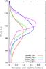 |
Fig. 7 Wind weighting functions computed assuming the adjusted atmospheric models described in Fig. 6, for a point on the equator at 8′′ from the sub-Earth point. |
We investigate here possible interpretations of the 2009 measurements in terms of wind field. The Doppler-shift maps (Fig. 5, middle and bottom panels) show a consistent pattern that is indicative of the main wind characteristics. The flow appears to globally circulate from sky-east to west, mimicking a zonal prograde wind that has seldom been observed on Venus and is unexpected from a physical point of view. Given the observing geometry, this could also correspond to a circulation from the day-side to the night-side, i.e. a SSAS wind. In the BN region, the flow direction is inverted, and corresponds to that of a retrograde zonal wind (RSZ). Along the central meridian longitude, the measured Doppler shifts are either very low or not significant, which argues for the absence of a measurable meridional wind. We therefore chose to only explore combinations of zonal and SSAS winds, using a single wind-field for the entire sounded altitude range. This approximate approach is motivated by the relatively low variation in the sounded altitude range across the disk (see Fig. 7). We did not try to adjust a given model for each individual Doppler-shift measurement but rather to build a global wind-field model capable of reproducing the observed Doppler-shift distribution as a whole.
To compute synthetic Doppler-shift maps for comparison to the observed data, we proceeded as follows: wind models were added to the radiative transfer model, by applying a Doppler shift (corresponding to the local line-of-sight projected wind) to the opacity spectra computed at every position on Venus’ disk for each altitude level. The planet’s own solid rotation (1.8 m/s at the equator) was neglected. The obtained models were transformed into synthetic visibilities with the same Fourier-plane coverage as the data. The models were then imaged and the line cores fitted using the procedure described in Sect. 3.3. In this manner, the synthetic models were produced and analyzed in precisely the same way as the data.
4.1. Zonal wind model
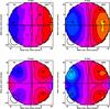 |
Fig. 8 Maps of synthetic Doppler shifts (in m/s), computed assuming different wind models. In each panel, Venus’ disk is represented by the centered circle, the synthesized beam by the ellipse in the bottom left hand corner, and the terminator by the vertical arc. The contour step corresponds to 20 m/s. The Fourier-plane coverage of June 12, 2009, was used to simulate the observations. Top-left panel: prograde zonal wind model with Veq = 69 m/s. Top-right panel: Bougher et al. (1986) SSAS wind model with Vter = 200 m/s. Bottom-left panel: Bougher et al. (1986) SSAS wind model with Vter = 200 m/s, combined with a Veq = 100 m/s RSZ wind, localized in an equatorial band. Bottom-right panel: same model as in bottom-left panel, but with a modified SSAS wind velocity field in the day-side varying as |
![Mathematical equation: \hbox{$V=V_{\rm ter}*\left(1-\big[\frac{\left|(90-sza)\right|}{90}\big]^5\right)$}](/articles/aa/full_html/2012/10/aa18451-11/aa18451-11-eq38.png)
Zonal winds are characterized as a longitudinal circulation at constant velocity for a given latitude, that can display variations with latitude and altitude.
We implemented a zonal prograde wind model, assuming that the wind mimics a solid rotation, i.e. with a velocity maximal at the equator and varying as cos(latitude) but no variation with altitude. We found that a 69 ± 14 m/s equatorial velocity for June 12 (75 ± 20 m/s respectively for June 13) can approximately match the observed limb-to-limb Doppler-shift difference, with the exception of the blue-night (BN) region (see Fig. 8, top-left panel). As discussed in Sect. 3.3, the 2007 data quality is insufficient to perform this analysis with the same confidence, but we note that the 2007 Doppler-shift pattern can be most accurately reproduced with a similar prograde zonal-wind speed (~85 m/s).
In the context of a zonal wind model, the approaching winds seen in the BN region can be interpreted as the signature of a localized retrograde zonal wind in an equatorial band between approximately 10° and −20° of latitude. The only possible explanation for this feature would be a change in the sounded altitude between the day-side and the night-side, which would also correspond to a change in the zonal wind direction. However, the altitude sounding estimates discussed in Sect. 3.4 show that the WWF for day and night conditions substantially overlap, and display a difference of 5 km at most for the maximal contribution layer. A radical change in the zonal wind direction in just over a scale height is unlikely, thus a combination of purely zonal winds is not a suitable hypothesis to explain the flow inversion in the BN region.
Even away from the BN region, the adjusted prograde zonal wind models are not entirely satisfactory. In these models, the increase in Doppler shift with longitude from sky-east to west is only due to the change in the projection factor, but the variation observed in the data on the day-side is more abrupt than the models near the central longitudes and shallower near the limbs. This indicates that the wind velocity on the day-side is not constant for a given latitude, but most likely increases from the limb to the central meridian (i.e. from the sub-solar region to the terminator). This argument again confirms that zonal winds alone are inappropriate to describe the observed wind field.
4.2. Sub-solar to anti-solar wind: model from Bougher et al. (1986)
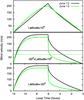 |
Fig. 9 Wind velocity as a function of local time for the best-fit parametrized wind models for different latitudinal regions (see Sect. 4.3 for details). The thick lines represent the SSAS wind velocity (plotted for an equivalent equator latitude), and the thin lines represent the RSZ wind velocity. Upper panel: models for latitudes >10°. Middle panel: models for latitudes between −20° and 10°. Lower panel: models for latitudes <–20°. |
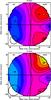 |
Fig. 10 Maps of synthetic Doppler shifts (in m/s) computed assuming the best-fit parametrized wind models, combining a modified SSAS wind-field and a localized RSZ wind. See Sect. 4.3 for a detailed description of these models. Top: model for June 12, 2009. Bottom: model for June 13, 2009. |
The thermospheric SSAS wind was modeled by Bougher et al. (1986) as a flow originating from the sub-solar point and following radial paths that are symmetric with respect to the SSAS line. The corresponding wind field is hence composed of both zonal and non-zonal components. The wind velocity, expressed as ![Mathematical equation: \hbox{$V=V_{\rm ter}*\left(1-[\frac{|(90-sza)|}{90}]\right)$}](/articles/aa/full_html/2012/10/aa18451-11/aa18451-11-eq45.png) , increases linearly with solar zenith angle (sza), being maximal at the terminator with velocity Vter. This model is commonly used as a tool to interpret mm-wave single-dish Doppler-shift data (see e.g. Lellouch et al. 2008; Sornig et al. 2011).
, increases linearly with solar zenith angle (sza), being maximal at the terminator with velocity Vter. This model is commonly used as a tool to interpret mm-wave single-dish Doppler-shift data (see e.g. Lellouch et al. 2008; Sornig et al. 2011).
We implemented this model taking into account the projection of the wind along the line of sight as presented in Shah et al. (1991) and Goldstein et al. (1991), and assuming no variations with altitude. If, as the model proposes, the SSAS wind velocity at the sub-solar and anti-solar longitudes is null, then the significant Doppler shifts measured at the limbs in these observations can only be explained by the combined effect of spatial beam convolution and a significant SSAS wind velocity at low solar zenith angle (solar incidence), implying very high maximal velocity at the terminator. By adjusting the maximal velocity, we find that assuming Vter = 200 ± 20 m/s for June 12 and Vter = 225 ± 25 m/s for June 13, SSAS wind models can globally reproduce the Doppler-shift maps far more accurately than zonal wind models (see Fig. 8, top-right panel). However they do not produce the flow inversion observed in the BN region. This feature could be interpreted as the signature of the return branch of the thermospheric SSAS wind that is expected to be present at lower altitudes than the SSAS flow, but was never unambiguously identified in previous observations. However, as shown in Fig. 7, the CO lines on the night-side tend to sound higher altitudes than on the day-side, which argues against this hypothesis. Hence the flow inversion cannot be explained in the context of a purely SSAS wind field.
Elsewhere, the match between the datasets and the models is similarly imperfect. In particular, the Bougher et al. (1986) SSAS model predicts a north-south and day-night symmetry of the wind-field, that is not observed. At southern latitudes (~40°), the best-fit model presented in Fig. 8 (top-right panel) indeed underestimates the Doppler shifts measured on the day-side, and overestimates Doppler shifts on the night-side, by a factor of up to four.
A SSAS wind is then mostly supported by the observations, but the multiple discrepancies between the model and the datasets show that the model proposed by Bougher et al. (1986) is, by itself, insufficient.
4.3. Descriptive model: SSAS wind and RSZ localized wind
As we have described in the two previous subsections, we inferred by using standard wind models to compare with the data, the following characteristics of the observed wind-field:
-
in the BN region, the flow inversion can be explained by a localRSZ wind;
-
the observations are globally consistent with a SSAS wind, but are also indicative of significant day-night and north-south asymmetries.
We explore hereafter combinations of RSZ localized winds with different SSAS wind models, assuming no variations with altitude.
Figure 8 (bottom-left panel) shows the example of a simple combination of a SSAS wind (Vter = 200 m/s, following the Bougher et al. (1986) model), with a RSZ wind (Veq = 100 m/s) limited to an equatorial band between −20° and 10° of latitude. This model succeeds in reproducing the wind inversion in the BN region, but, as the model is symmetric with respect to the terminator, also displays a wind inversion feature near the sub-solar region, that is at odds with the observations. The zonal wind velocity being, by definition, constant with longitude, the only way to get around this is to introduce day/night asymmetries in the SSAS wind field. More precisely, near the equator, the SSAS wind needs to be stronger in the sub-solar region than in the anti-solar region. In this manner, the SSAS wind (resp. RSZ) dominates in the sub-solar region (resp. anti-solar region).
We introduce this asymmetry by modifying the SSAS wind-field on the day hemisphere. The proposed model is identical to the previous model with the exception that, on the day hemisphere, the SSAS wind velocity varies as ![Mathematical equation: \hbox{$V=V_{\rm ter}*\left(1-[\frac{|(90-sza)|}{90}]^5\right)$}](/articles/aa/full_html/2012/10/aa18451-11/aa18451-11-eq48.png) . This allows the SSAS wind velocity to drop less quickly away from the terminator, such that the SSAS wind is still significant even close to the eastern limb (sub-solar region). As a result, as shown in Fig. 8 (bottom-right panel), the wind inversion is now detected only near the anti-solar region, as in the observations. However satisfying, this model can still be adjusted so as to account for the remaining discrepancies to the data, that are mainly associated with observed asymmetries between northern and southern hemispheres.
. This allows the SSAS wind velocity to drop less quickly away from the terminator, such that the SSAS wind is still significant even close to the eastern limb (sub-solar region). As a result, as shown in Fig. 8 (bottom-right panel), the wind inversion is now detected only near the anti-solar region, as in the observations. However satisfying, this model can still be adjusted so as to account for the remaining discrepancies to the data, that are mainly associated with observed asymmetries between northern and southern hemispheres.
To provide the closest match to the data, we added to the previous model a latitudinal asymmetry in the SSAS wind-field, and used a parametrized expression to describe the SSAS wind velocity as ![Mathematical equation: \hbox{$V=V_{\rm ter}*\left(1-[\frac{|(90-sza)|}{90}]^X\right)$}](/articles/aa/full_html/2012/10/aa18451-11/aa18451-11-eq49.png) . At latitudes higher than 10° north, the best-fit SSAS wind model appears to be very similar to the Bougher et al. (1986) model, with only little day/night asymmetry. For June 12, the best results are obtained with X = 1 on the day-side and X = 0.8 on the night-side (resp. X = 1.5 and X = 1 on June 13). In contrast, for latitudes below 10° north, the best-fit SSAS wind model flows quickly on the day-side hemisphere, even close to the sub-solar region, and sharply slows down past the terminator on the night-side hemisphere. This translates into a large variation in the X parameter between the day and night hemispheres. The best-fit results for June 12 are obtained for X = 5 on the day-side and X = 0.45 on the night-side (resp. X = 5 and X = 0.15 on June 13). The best-fits for the SSAS terminator velocity are obtained for Vter = 220 m/s (resp. Vter = 200 m/s), and, for the equatorial RSZ wind velocity, Veq = 100 m/s (resp. Veq = 70 m/s). The best-fit wind models are graphically summarized in Fig. 9, and the corresponding Doppler-shift maps are represented in Fig. 10.
. At latitudes higher than 10° north, the best-fit SSAS wind model appears to be very similar to the Bougher et al. (1986) model, with only little day/night asymmetry. For June 12, the best results are obtained with X = 1 on the day-side and X = 0.8 on the night-side (resp. X = 1.5 and X = 1 on June 13). In contrast, for latitudes below 10° north, the best-fit SSAS wind model flows quickly on the day-side hemisphere, even close to the sub-solar region, and sharply slows down past the terminator on the night-side hemisphere. This translates into a large variation in the X parameter between the day and night hemispheres. The best-fit results for June 12 are obtained for X = 5 on the day-side and X = 0.45 on the night-side (resp. X = 5 and X = 0.15 on June 13). The best-fits for the SSAS terminator velocity are obtained for Vter = 220 m/s (resp. Vter = 200 m/s), and, for the equatorial RSZ wind velocity, Veq = 100 m/s (resp. Veq = 70 m/s). The best-fit wind models are graphically summarized in Fig. 9, and the corresponding Doppler-shift maps are represented in Fig. 10.
These models provide a very close match to the observed Doppler-shift distribution, but a global circulation modeling would be required to check whether these spatial variations are theoretically possible and justified. In addition, these are certainly not the unique wind-field solution that could reproduce the observations. It is then difficult to quantify the temporal variations that can be derived from the observations. It is safe to say that, in the context of the proposed models, the velocity of the winds (both RSZ and SSAS) varies by as much as 30 m/s, although the wind-field structure does not change in the 24 h separating the two observations.
5. Summary and discussion
We have presented observations of the CO(1–0) line on Venus obtained at the IRAM-Plateau de Bure interferometer in November 2007 and June 2009. Our measurements of the Doppler shifts in the line core have enabled us to map the upper mesosphere wind field on the morning hemisphere with a spatial resolution (3.5–5.5′′), which is much higher than those reached with single-dish facilities. Using atmospheric models based on line-shape fitting, we have determined that the winds detected primarily sound altitudes between 96 km and 101 km.
The Doppler-shift maps obtained reveal that the wind mostly follows a sky-east to west direction, corresponding in the observed geometry to the SSAS wind direction. No significant meridional winds could be detected. In addition, an inversion of the flow direction was measured on the night-side near the equator. In 2009, the remarkable temporal stability between the two observing dates and the very high data quality helps us to have strong confidence in these results. The observations obtained in 2007 are of much lower quality mainly because of their poor imaging quality related to the near 0° declination of the target, and could not be analyzed in detail. The obtained wind pattern however suggests some similarities with the 2009 data.
To provide the most accurate description of the wind field observed in 2009, we compared our results to a series of wind models. The best results were obtained with a global, dominant SSAS wind combined with an equatorial localized RSZ wind. Our proposed SSAS wind model includes significant asymmetries between the day and night hemispheres, as well as latitudinal variations. In particular, at latitudes lower than 10°, the SSAS wind velocity decreases slowly across the disk from the terminator to the sub-solar region (day hemisphere), but decreases quickly from the terminator to the anti-solar region (night hemisphere). Analyses of observations by Lellouch et al. (2008) and Clancy et al. (2011) also found evidence of latitudinal variations in the SSAS wind-field but in a very different, latitudinally symmetric form, while our models appear to provide evidence of significant north/south asymmetries.
Our SSAS wind model thus differs from the most commonly used model of Bougher et al. (1986), which proposes a linear variation in the wind velocity with solar incidence all over the disk. We note that, although the wind model of Bougher et al. (1986) is based on the observational constraints of composition and temperature distribution measured by Pioneer above 100 km, this model has never been directly observationally confirmed. Airglow tracking (Hueso et al. 2008) and mm-wave Doppler-shift mapping (Clancy et al. 2011) also revealed significant discrepancies between the observed wind field and the Bougher et al. (1986) model.
The best-fit models were found for maximal SSAS wind velocities at the terminator of 200–220 m/s, which are comparable to the sound speed (200 m/s) but higher than most velocities estimated by previous works at this altitude, usually of the order of ~100 m/s. However, the same previous studies did also find very large temporal variations in the SSAS wind velocity. Very high terminator velocities (290–322 m/s at 102 km) are compatible with the data presented in Lellouch et al. (2008), although they were not the favored solution. The SSAS modified wind model presented by Clancy et al. (2011) is also characterized by low-latitude terminator velocities of ~200 m/s at 108 km altitude. The velocities derived from this paper therefore seem plausible in the context of previous studies.
Finally, our models propose the coexistence of a RSZ wind localized in an equatorial band (at latitudes between −20° and 10°), whose velocity at the equator varies between 70–100 m/s. The presence of a RSZ wind agrees with most observations of the upper mesosphere dynamics (mm-wave and IR Doppler-shift mapping, airglow and minor species distribution), where the SSAS wind is dominant and coexists with a very temporally variable RSZ wind. However, the RSZ wind detected here is very spatially localized, a result that has never been derived from other observations. Only moderate variations in the zonal wind velocity with latitude have been previously observed, for example in Sornig et al. (2008, 2011).
Small temporal variations in the winds velocity by ~30 m/s were also detected in both the SSAS wind and the RSZ wind in the 24-h time span between the two 2009 observations, which is remarkably stable, since very large variations (of up to 140 m/s for the RSZ wind and 60 m/s for the SSAS wind) could be observed on a similar timescale by Clancy et al. (2011), and even more radical changes in the wind structure can be monitored on longer timescales.
Although not unambiguous, our interpretation of the wind field observed in 2009 agrees with the usual picture of the upper mesosphere dynamics (combination of SSAS and RSZ winds), but at the same time clearly indicates that the wind field structure is more complicated than the usual adopted models. This work demonstrates the ability of mm-wave interferometry to characterize a wind field, on a larger spatial scale and with an easier interpretation than the airglow tracking method. To describe the wind field on a planet-wide scale and constrain the long-term stability of the wind structures, observations at other Venusian phases will be needed, especially near superior conjunction, when the entire day-side disk is sampled and Venus’ apparent size is minimal (~10′′). Future studies accessible with
the Atacama Large Millimeter Array (ALMA) may include both high spatial resolution mapping (~1′′), which would permit us to explore the dynamics in the high latitude regions, and short timescale (~1 h) monitoring to detect quick changes in the wind structure and velocity.
Acknowledgments
Arielle Moullet is a Jansky Fellow of the National Radio Astronomy Observatory. The National Radio Astronomy Observatory is a facility of the National Science Foundation operated under cooperative agreement by Associated Universities, Inc. We thank T. Clancy for providing us with the reference atmospheric profiles. We acknowledge the commitment of the staff at IRAM-PdBI in performing these challenging observations. IRAM is supported by INSU/CNRS (France), MPG (Germany), and IGN (Spain).
References
- Bougher, S. W., Dickinson, R. E., Ridley, E. C., et al. 1986, Icarus, 68, 284 [NASA ADS] [CrossRef] [Google Scholar]
- Bougher, S. W., Alexander, M. J., & Mayr, H. G. 1997, in Venus II: Geology, Geophysics, Atmosphere, and Solar Wind Environment, eds. S. W. Bougher, D. M. Hunten, & R. J. Phillips, 259 [Google Scholar]
- Clancy, R. T., & Muhleman, D. O. 1985, Icarus, 64, 157 [NASA ADS] [CrossRef] [Google Scholar]
- Clancy, R. T., Sandor, B. J., & Moriarty-Schieven, G. H. 2003, Icarus, 161, 1 [NASA ADS] [CrossRef] [Google Scholar]
- Clancy, R. T., Sandor, B. J., & Moriarty-Schieven, G. H. 2008, Planet. Space Sci., 56, 1344 [NASA ADS] [CrossRef] [Google Scholar]
- Clancy, T., Sandor, B., & Moriarty-Schieven, G. 2011, Icarus, accepted [Google Scholar]
- de Pater, I., Schloerb, F. P., & Rudolph, A. 1991, Icarus, 90, 282 [NASA ADS] [CrossRef] [Google Scholar]
- Gérard, J., Saglam, A., Piccioni, G., et al. 2008, Geophys. Res. Lett., 35 [Google Scholar]
- Gierasch, P. J., Goody, R. M., Young, R. E., et al. 1997, in Venus II: Geology, Geophysics, Atmosphere, and Solar Wind Environment, eds. S. W. Bougher, D. M. Hunten, & R. J. Phillips, 459 [Google Scholar]
- Goldstein, J. J., Mumma, M. J., Kostiuk, T., et al. 1991, Icarus, 94, 45 [NASA ADS] [CrossRef] [Google Scholar]
- Gurwell, M. A., Muhleman, D. O., Shah, K. P., et al. 1995, Icarus, 115, 141 [NASA ADS] [CrossRef] [Google Scholar]
- Högbom, J. A. 1974, A&AS, 15, 417 [NASA ADS] [Google Scholar]
- Hueso, R., Sánchez-Lavega, A., Piccioni, G., et al. 2008, J. Geophys. Res. (Planets), 113 [Google Scholar]
- Kasprzak, W. T., Keating, G. M., Hsu, N. C., et al. 1997, in Venus II: Geology, Geophysics, Atmosphere, and Solar Wind Environment, eds. S. W. Bougher, D. M. Hunten, & R. J. Phillips, 225 [Google Scholar]
- Lellouch, E., Goldstein, J. J., Rosenqvist, J., Bougher, S. W., & Paubert, G. 1994, Icarus, 110, 315 [NASA ADS] [CrossRef] [Google Scholar]
- Lellouch, E., Paubert, G., Moreno, R., & Moullet, A. 2008, Planet. Space Sci., 56, 1355 [NASA ADS] [CrossRef] [Google Scholar]
- Limaye, S. S. 2007, J. Geophys. Res. (Planets), 112, 4 [CrossRef] [Google Scholar]
- Markiewicz, W. J., Titov, D. V., Limaye, S. S., et al. 2007, Nature, 450, 633 [NASA ADS] [CrossRef] [Google Scholar]
- Moissl, R., Khatuntsev, I., Limaye, S. S., et al. 2009, J. Geophys. Res. (Planets), 114 [Google Scholar]
- Moreno, R., Lellouch, E., Forget, F., et al. 2009, Icarus, 201, 549 [NASA ADS] [CrossRef] [Google Scholar]
- Moullet, A., Lellouch, E., Moreno, R., Gurwell, M. A., & Moore, C. 2008, A&A, 482, 279 [NASA ADS] [CrossRef] [EDP Sciences] [Google Scholar]
- Piccialli, A. 2010, Ph.D. Thesis, ESA, ESTEC [Google Scholar]
- Piccialli, A., Titov, D. V., Grassi, D., et al. 2008, J. Geophys. Res. (Planets), 113 [Google Scholar]
- Sánchez-Lavega, A., Hueso, R., Piccioni, G., et al. 2008, Geophys. Res. Lett., 35 [Google Scholar]
- Shah, K. P., Muhleman, D. O., & Berge, G. L. 1991, Icarus, 93, 96 [NASA ADS] [CrossRef] [Google Scholar]
- Sornig, M., Livengood, T., Sonnabend, G., et al. 2008, Planet. Space Sci., 56, 1399 [NASA ADS] [CrossRef] [Google Scholar]
- Sornig, M., Livengood, T., Sonnabend, G., Stupar, D., & Kroetz, P. 2011, Icarus, accepted [Google Scholar]
- Steer, D. G., Dewdney, P. E., & Ito, M. R. 1984, A&A, 137, 159 [NASA ADS] [Google Scholar]
- Widemann, T., Lellouch, E., & Campargue, A. 2007, Planet. Space Sci., 55, 1741 [NASA ADS] [CrossRef] [Google Scholar]
- Widemann, T., Lellouch, E., & Donati, J. 2008, Planet. Space Sci., 56, 1320 [NASA ADS] [CrossRef] [Google Scholar]
All Tables
All Figures
|
Fig. 1 Aspect of Venus on November 16, 2007 (top) and June 12, 2009 (bottom). The black dot next to the eastern limb represents the sub-solar point. The small circle at the center represents the sub-earth point. Coordinates of the sub-earth and sub-solar points are indicated in the east longitude convention, along with the pole axis tilt angle. From http://www.imcce.fr |
| In the text | |
|
Fig. 2 Continuum visibilities obtained in November 2007 (top panels, merged data from the two observing dates) and June 2009 (bottom panels, data from June 13). Left panels: amplitude (in Jy) of the visibilities, plotted against projected baseline length (in meters). Right panels: corresponding Fourier-plane coverage. The units correspond to the component of the projected baselines in the east-west (U) and north-south (V) directions (in m). |
| In the text | |
|
Fig. 3 Maps of Venus’ CO(1–0) spectra (in Jy/beam), for different observing dates. The location of each spectrum with respect to the disk center is indicated in parenthesis (in arcseconds). The velocity scale for each individual spectrum goes from −2 to + 2 km s-1. The continuum level is represented by the blue background. In each panel, Venus’ disk is represented by the centered circle, the synthesized beam by the ellipse in the bottom left hand corner, and the terminator by the vertical arc. The maps were rotated so that the pole axis is vertical in the figure. Top panel: 2007 observations (merged data from the two observing dates). The flux scale goes from 0 to 75 Jy/beam. Middle panel: June 12, 2009 observations. The flux scale goes from 0 to 75 Jy/beam. Bottom panel: June 13, 2009 observations. The flux scale goes from 0 to 120 Jy/beam. |
| In the text | |
|
Fig. 4 CO(1–0) lines measured on June 12, 2009, plotted against synthetic lines computed assuming adjusted atmospheric models. Model 1 (for day and night conditions) corresponds to a model where only the temperature profile is adjusted, while the CO mixing profile is fixed to the reference profile. Model 2 (for day and night conditions) corresponds to a model where only the CO mixing profile is adjusted, while the temperature profile is fixed to the reference profile. Top: day-side spectra measured on the equator at 8′′ from the sub-earth point (9.3 am local time). Bottom: night-side spectra measured on the equator at 8′′ from the sub-earth point (3.1 am local time). |
| In the text | |
|
Fig. 5 Maps of the Doppler shifts (in m/s) measured in the core of the CO(1–0) lines, for different observing dates. Regions where Doppler shifts could not be retrieved appear as blank. In each panel, Venus’ disk is represented by the centered circle, the synthesized beam by the ellipse in the bottom left-hand corner, and the terminator by the vertical arc. The contour step corresponds to 20 m/s. The maps were rotated to ensure that the pole axis is vertical in the figure. Top panel: 2007 observations (merged data from the two observing dates). Doppler-shift errors are on the order of 25–35 m/s on the day-side and 15–20 m/s on the night-side. Middle panel: June 12, 2009 observations. Errors are on the order of 10 m/s on the day-side and 6 m/s on the night-side. Bottom panel: June 13, 2009 observations. Errors are on the order of 15–22 m/s on the day-side and 7 m/s on the night-side. |
| In the text | |
|
Fig. 6 Atmospheric models adjusted to the CO(1–0) lines represented in Fig. 4. Left: CO mixing ratio profiles. Right: temperature profiles. |
| In the text | |
|
Fig. 7 Wind weighting functions computed assuming the adjusted atmospheric models described in Fig. 6, for a point on the equator at 8′′ from the sub-Earth point. |
| In the text | |
|
Fig. 8 Maps of synthetic Doppler shifts (in m/s), computed assuming different wind models. In each panel, Venus’ disk is represented by the centered circle, the synthesized beam by the ellipse in the bottom left hand corner, and the terminator by the vertical arc. The contour step corresponds to 20 m/s. The Fourier-plane coverage of June 12, 2009, was used to simulate the observations. Top-left panel: prograde zonal wind model with Veq = 69 m/s. Top-right panel: Bougher et al. (1986) SSAS wind model with Vter = 200 m/s. Bottom-left panel: Bougher et al. (1986) SSAS wind model with Vter = 200 m/s, combined with a Veq = 100 m/s RSZ wind, localized in an equatorial band. Bottom-right panel: same model as in bottom-left panel, but with a modified SSAS wind velocity field in the day-side varying as |
| In the text | |
|
Fig. 9 Wind velocity as a function of local time for the best-fit parametrized wind models for different latitudinal regions (see Sect. 4.3 for details). The thick lines represent the SSAS wind velocity (plotted for an equivalent equator latitude), and the thin lines represent the RSZ wind velocity. Upper panel: models for latitudes >10°. Middle panel: models for latitudes between −20° and 10°. Lower panel: models for latitudes <–20°. |
| In the text | |
|
Fig. 10 Maps of synthetic Doppler shifts (in m/s) computed assuming the best-fit parametrized wind models, combining a modified SSAS wind-field and a localized RSZ wind. See Sect. 4.3 for a detailed description of these models. Top: model for June 12, 2009. Bottom: model for June 13, 2009. |
| In the text | |
Current usage metrics show cumulative count of Article Views (full-text article views including HTML views, PDF and ePub downloads, according to the available data) and Abstracts Views on Vision4Press platform.
Data correspond to usage on the plateform after 2015. The current usage metrics is available 48-96 hours after online publication and is updated daily on week days.
Initial download of the metrics may take a while.