| Issue |
A&A
Volume 544, August 2012
|
|
|---|---|---|
| Article Number | A139 | |
| Number of page(s) | 6 | |
| Section | The Sun | |
| DOI | https://doi.org/10.1051/0004-6361/201219670 | |
| Published online | 14 August 2012 | |
X-ray emitting hot plasma in solar active regions observed by the SphinX spectrometer
1
Dipartimento di FisicaUniversità di Palermo,
Piazza del Parlamento 1,
90134
Palermo,
Italy
e-mail: This email address is being protected from spambots. You need JavaScript enabled to view it.
2
INAF – Osservatorio Astronomico di Palermo, Piazza del Parlamento
1, 90134
Palermo,
Italy
3
Space Research Centre, Polish Academy of Sciences,
51-622, Kopernika
11, Wrocław,
Poland
Received: 24 May 2012
Accepted: 17 July 2012
Abstract
Aims. The detection of very hot plasma in the quiescent corona is important for diagnosing heating mechanisms. The presence and the amount of such hot plasma is currently debated. The SphinX instrument on-board the CORONAS-PHOTON mission is sensitive to X-ray emission of energies well above 1 keV and provides the opportunity to detect the hot plasma component.
Methods. We analysed the X-ray spectra of the solar corona collected by the SphinX spectrometer in May 2009 (when two active regions were present). We modelled the spectrum extracted from the whole Sun over a time window of 17 days in the 1.34−7 keV energy band by adopting the latest release of the APED database.
Results. The SphinX broadband spectrum cannot be modelled by a single isothermal component of optically thin plasma and two components are necessary. In particular, the high statistical significance of the count rates and the accurate calibration of the spectrometer allowed us to detect a very hot component at ~7 million K with an emission measure of ~2.7 × 1044 cm-3. The X-ray emission from the hot plasma dominates the solar X-ray spectrum above 4 keV. We checked that this hot component is invariably present in both the high and low emission regimes, i.e. even excluding resolvable microflares. We also present and discuss the possibility of a non-thermal origin (which would be compatible with a weak contribution from thick-target bremsstrahlung) for this hard emission component.
Conclusions. Our results support the nanoflare scenario and might confirm that a minor flaring activity is ever-present in the quiescent corona, as also inferred for the coronae of other stars.
Key words: Sun: corona / methods: observational / techniques: spectroscopic
© ESO, 2012
1. Introduction
The solar corona is X-ray bright. The bulk of its emission is thermal, and its spectrum is made of a multitude of emission lines, e.g. of iron, overlapping a bremsstrahlung continuum, which is characteristic of an optically thin plasma at 1−3 MK. Most of the emission comes from plasma confined in closed magnetic tubes anchored in the photosphere, the so-called coronal loops. Hotter plasma, with temperatures well above 10 MK, is typically detected during very impulsive flare events occurring in localized coronal regions.
The high sensitivity of new imaging and spectral instrumentation has recently allowed us to refine the investigation of the thermal structure of the corona. One question is whether there is a very hot component at temperatures above 6−8 MK, even outside macroscopic flare events. This question is linked to the more basic question of whether there is flaring activity down to very small scales, that constitutes a major steady component of the heating, extending into the entire solar corona. Although very faint, such a component has been recently detected in active regions both with either filter ratios or differential emission measure (DEM) reconstruction performed by imaging broad-band instruments (Hinode/XRT, e.g., Reale et al. 2009a,b; McTiernan 2009; Schmelz et al. 2009) and spectroscopic line analyses (single-line or DEM reconstruction, e.g., Ko et al. 2009; Patsourakos & Klimchuk 2009; Shestov et al. 2010; Sylwester et al. 2010). More solid confirmation has very recently been found (Testa & Reale 2012). The weight of this very hot component has been estimated to be a few percent at most of the major component around 3 MK in an active region (Reale et al. 2009a). However, there are reasons to believe that the amount of very hot plasma may vary from one active region to another and that it may be smaller in less prominent active regions (e.g. Testa et al. 2011).
Another poorly constrained quantity is the weight of this hot component over long timescales and relative to the global coronal budget. Some hints were provided by the Sun-as-a-star analysis with Yohkoh data (Argiroffi et al. 2008), which, however, had large uncertainties in the emission measure of the hotter plasma. Tighter constraints are therefore needed in the hot tail.
The Solar PHotometer IN X-rays (SphinX; Sylwester et al. 2008; Gburek et al. 2011), which was part of the THESIS package on-board the CORONAS-PHOTON solar mission, is appropriate for investigating this issue: it was a broad-band spectrometer (1−15 keV), with moderate spectral resolution but sensitive up to high energies,which is enough to detect any small hot components. Sylwester et al. (2012; hereafter SKG12) analysed coronal spectra measured with SphinX at the last solar minimum, finding that they are well-described by a thermal spectrum at about 1.7−1.9 MK, with significant flux only in the 1−3 keV range.
Here we analyse the full-disk unresolved corona during a low solar-activity period but in the presence of active regions, to search for any minor hot component. In this analysis, we take advantage of our ability to integrate over several observation days. This allows us to achieve a very high signal-to-noise ratio and access the high energy band (>3 keV), where the steep coronal spectrum has a very low count rate, but which is crucial to detect any hot component.
Although we include active regions in the analysis, we address the non-flaring corona and we exclude any major flare event in the data selection. We discuss the role of any minor, still resolved, flaring components (microflares).
Going to these high energies, one may wonder about the possible role of non-thermal emission. High-energy spectral components are for instance typically detected during flares with RHESSI (e.g. Veronig et al. 2006; Krucker et al. 2008). In the case of lower activity, we may hope in principle to detect non-thermal emission in the SphinX spectral range. We therefore investigate also this issue.
The paper is organized as follows: in Sect. 2, we describe the data and the data analysis procedure; in Sect. 3, we show the results of the spectral analysis (and of the count-rate resolved spectral analysis). Our conclusions are discussed in Sect. 4.
2. Data analysis
The spectra presented in this paper were collected by the D1 detector of the SphinX spectrometer. The detector energy range is 1.2−14.9 keV and the spectral resolution is ~460 eV. Further details on the instrumental characteristics can be found in Gburek et al. (2011) and SKG12.
We considered all the observations between 2009 May 7 and 2009 May 241. The choice of this time window was dictated by the relatively high solar X-ray flux (associated with active regions) and the lack of significant flaring events. The active region AR11017 (hereafter AR1) was visible between May 7 and 22, while a second, dimmer, active region (hereafter AR2) was visible from May 15 to the end of our time window. Figure 1 shows the Hinode/XRT synoptic images of the Sun (Ti-poly filter) on May 7, May 15, and May 23, together with the corresponding positions of AR1 and AR2.
To reduce any contamination from solar flares, we carefully inspected the light-curves of all the observations and excluded observations SPHINX_090509_192730_254950 and SPHINX_090514_062135_064952 to remove a B1.0 and a A5.9 flare, respectively.
 |
Fig. 1 Hinode/XRT synoptic images of the solar corona (Ti-poly filter) in 2009 May 7 (upper panel), 2009 May 15 (central panel), and 2009 May 23 (lower panel). The position of active regions AR1 and AR2 is marked. |
For each event file, we extracted the corresponding spectrum by applying a very conservative screening criterium to remove particle-related events, spurious mesurements, and non-GTI events. Namely, we selected FLAG = 0 events only (see the SphinX web site for a detailed description of individual flags). We then summed the single spectra to obtain a total spectrum with more than 3.9 × 10⁷ counts and 57 ks of filtered exposure time.
We adopted the response matrix SPHINX_RSP_256_nom_ D1.fts and performed spectral analysis by using XSPEC V12.7 (Arnaud 1996). We performed gain fits within Xspec to account for possible weak variations in the response gain produced by fluctuations in the detector temperature during the 17 days spanned by our observations. This procedure shifts the energies E for which the response matrix is defined according to the formula E′ = (E/g1) − g2, where (g1,g2) are free parameters in the fit. For all the models described below, we found that g1 ~ 1.025, and g2 ~ −0.03, in agreement with expectations for small variations in the response matrix.
Spectral analysis was performed in the 1.34−7 keV energy band (i. e. instrument channels 24−121) to minimize calibration issues (1.2−1.34 keV) and contaminations from the electronic noise (7−14.9 keV). The total spectrum was modelled by adopting the APEC spectral code (optically thin coronal plasma in collisional ionization equilibrium, Smith et al. 2001) based on the 2.0 release of the AtomDB database2. Because of the relatively limited SphinX spectral resolution, it was impossible to clearly identify line emission features in the spectra and perform accurate diagnostics of the abundances. We therefore set the abundance table in the spectral model to that reported by Feldman (1992) for the solar upper atmosphere. We added a systematic 5% error term in our spectral fittings to account for the estimated uncertainties in the calibration of the spectrometer.
3. Results
We first verified that the total SphinX broad-band spectrum cannot be properly described by a single isothermal component. A fit of this simple model to the spectrum provides an unacceptable reduced χ2 = 7.06 (with 93 d.o.f.) and significant residuals are visible in the high-energy tail of the spectrum, as shown in the upper panel of Fig. 2.
The SphinX spectrum can be well-fitted by adding a second thermal component (see middle panel of Fig. 2). The model with two components provides a reduced χ2 = 1.07 (with 91 d.o.f.) and a null hypothesis probability >30%. The 1−8 Å X-ray flux is 1.4 × 10⁻⁵ erg/s/cm2 and the 1−15 keV luminosity is 4.7 × 10²³ erg/s. Table 1 shows the best-fit parameters obtained with one and two thermal components. We did not obtain significant improvements to the quality of the fits by adding a further thermal component. In particular, according to the F-test, the probability that the improvement in the fit is insignificant is more than three times higher than our threshold at 0.1% and the error bars in the best-fit parameters are larger. We therefore conclude that the broadband modelling of the SphinX spectrum requires two thermal components, a warm component at ~2.7 × 10⁶ K and a hot one ~7 × 10⁶ K (hereafter 2T model).
Best-fit parameters obtained by modelling the SphinX spectrum with one (1T) and two (2T) isothermal components of optically thin plasma, and with one thermal component plus a power-law (1T-Pow).
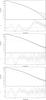 |
Fig. 2 Upper panel: SphinX spectrum of the solar corona collected between 2009 May 7 and 2009 May 24, together with its best-fit model consisting of one isothermal component and residuals. Middle panel: same as upper panel with a two-component thermal model. The contribution of each component is shown. Lower panel: same as middle panel with the 1T-Pow model. |
The high-energy tail of the SphinX spectrum can also be fitted by a non-thermal component. A model with a (warm) thermal component plus a power-law (1T-Pow model, see lower panel of Fig. 2) provides a χ2 = 94.0 (with 91 d.o.f.) that is even lower than that obtained with the 2T model. In this case, the values of T1 and EM1 are consistent with those obtained with the 2T model, while for the non-thermal component we obtain a quite steep photon index Γ, as shown in Table 1. Therefore, with the available data it is impossible to exclude that the hard X-ray emitting component is associated with non-thermal processes and/or is a combination of thermal and non-thermal emission.
SKG12 analysed SphinX spectra extracted from the lowest-activity periods of the 2009 solar minimum and characterized by a lack of major active regions. They found that in time intervals of exceptionally low X-ray flux, SphinX spectra can be modelled by a single thermal component at 1.7−1.9 × 10⁶ K with emission measure ranging between 4 × 1047 cm-3 and 1.1 × 1048 cm-3. We note that in the spectra studied by SKG12 the 1−15 keV X-ray luminosity is a factor of 6−10 lower than that in our spectrum. The differences in the X-ray luminosity, plasma temperature, and spectral model can be related to active regions AR1 and AR2 in our observations. We examined the Hinode/XRT synoptic images of the Sun in the thin−Be filter, whose bandwidth is approximatively 0.9−2.5 keV (three observations being available in our time window for May 16, 19, and 20) and found that the contribution (in terms of Digital Numbers, DN, detected by XRT) of AR1 and AR2 is only ~6−9% of the total. Therefore, the contribution of the active regions to the total flux dominates only at high energy.
In principle, it is possible to ascertain the contribution of AR1 and AR2 by assuming that the spectrum of the underlying corona is described by the model adopted by SKG12. Under this assumption, one can add a third, cooler, component to the 2T model (by forcing in the fitting process that its temperature, T0, and its emission measure, EM0, are in the ranges derived by SKG12). Unfortunately, this approach is unfeasible since, as explained above, the addition of a new component leads to less precise measures of the best-fit parameters. Nevertheless, this 3T model yields T0 ~ 1.9 × 10⁶ K and EM0 ~ 1 × 1048 cm-3, while T1, T2, EM1, and EM2 are all consistent with those reported in Table 1 to within one sigma (but with much larger uncertainties).
The upper panel of Fig. 3 shows the 68%, 90%, and 99% confidence contour levels of the emssion measure of the warm component, EM1, versus the emission measure of the hot component EM2. The contours indicate that the ratio EM1/EM2 is almost constant at ~2500. The best-fit value of T2 is entangled with EM2, as shown by the 68%, 90%, and 99% confidence contour levels in the lower panel of Fig. 3.
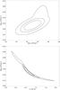 |
Fig. 3 Upper panel: the 68%, 90%, and 99% confidence contour levels of the emssion measure of the hot component, EM2, versus the emission measure of the warm component EM1 obtained with the 2T model. Lower panel: same as upper panel for EM2 and T2. |
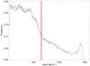 |
Fig. 4 Distribution of the X-ray count-rate observed by SphinX between 2009 May 7 and 2009 May 24. The red vertical line indicates the threshold chosen to extract the low count-rate spectrum and the high count-rate spectrum (see text). |
3.1. Count-rate resolved spectral analysis
Figure 4 shows the distribution of the X-ray count-rate observed by SphinX in our 17 day time window. The average count-rate is a few hundreds of counts s-1, but a peak at ~1400 counts s-1 is also visible. The peak at high count-rate may be associated with microflares not directly visible through a simple inspection of the light curve. These microflares may also be responsible for the hot component detected in the solar spectrum. To investigate this issue, we performed a count-rate resolved spectral analysis by extracting the spectrum of all the events detected at low count-rate (<650 s-1, hereafter LR spectrum) and the spectrum of all the events detected at high count-rate (>650 s-1, HR spectrum). Figure 5 shows the LR and HR spectra.
 |
Fig. 5 SphinX spectrum of all the events detected at low count-rate (<650 s-1, black crosses) and at high count-rate (>650 s-1 red crosses) between 2009 May 7 and 2009 May 24. |
We found a clear relationship between count-rate and spectral hardness, with the HR spectrum being significantly harder than the LR spectrum. In particular, the soft (1.34−3 keV) to hard (3−7 keV) flux ratio is ~1000 in the LR spectrum and ~500 in the HR spectrum. This result supports a possible link between high count-rate and microflare activity. Nevertheless, though the LR spectrum is softer than the HR spectrum, the former cannot be modelled by a single thermal component (reduced χ2 = 3.57 with 93 d.o.f.) and a proper fit still requires either an additional hot component (reduced χ2 = 0.98 with 91 d.o.f.) or a power-law (reduced χ2 = 1.01 with 91 d.o.f.). This clearly proves that the hot component cannot be only an effect of microflares, since it is present even in regimes of low count-rate, where any contamination from microflares is removed.
Table 2 shows the best-fit parameters obtained by fitting the LR and HR spectra with one and two thermal components, and with one thermal component plus a power-law. Because of the lower statistical significance of the count rates, error bars are somehow larger than those obtained for the total spectrum and we still found an entanglement between the best-fit values of EM2 and T2 (similar as shown in Fig. 3). Table 2 shows that the best-fit temperatures obtained for the HR spectrum are higher than those obtained for the LR spectrum (and from those obtained for the total spectrum, see Table 1). This is coherent with the HR spectrum having harder X-ray emission.
Best-fit parameters obtained by modelling the LR and HR spectra (see text) with one (1T) and two (2T) isothermal components of optically thin plasma, and with one thermal component plus a power-law (1T-Pow).
4. Discussion and conclusions
We have illustrated the analysis of full-disk X-ray data collected with the SphinX spectrometer over a two-week period when one or two active regions were present on the solar disk. Although SphinX has no spatial resolution, its wide energy coverage and sensitivity up to high X-ray energies (>10 keV) make it suited to investigating the presence and role of high temperature plasma components in the solar corona.
Although the solar X-ray spectrum is quite steep, integrating over two weeks allowed us to reach a very high signal-to-noise ratio well above 3 keV. This represented a significant improvement on previous studies. We analysed such a broad-band spectrum, with one and two-thermal component models, finding that the spectrum is not well-described by a single thermal component and that a second hotter component improves the fitting at a high significance level. In addition to the large warm component previously found in the very quiet Sun, which we confirm exists here (T ≈ 2.7 MK), our analysis has detected a minor hot component (T ≈ 7 MK) at extremely high significance. The X-ray emission from the hot plasma dominates the solar X-ray spectrum above 4 keV and is clearly associated with the active regions, which were absent in the analysis of SKG12. The temperature of this hot component is compatible with that found in other studies of active regions (Reale et al. 2009a; Testa et al. 2011). The results of present investigations also agree with the multitemperature analysis (DEM reconstruction) based on the 15 line fluxes observed by the RESIK spectrometer in the range 3.5−6 Å (Sylwester et al. 2010): the examination of non-flaring periods (activity classes from A9 to B5) at the beginning of 2003 indicated that the temperatures of hot DEM component are between 6 MK and 9 MK and that its emission measure is three orders of magnitude smaller than that of the cooler component.
Our fittings show that the emission measure of the hotter component is <0.1% of the other cooler one. As mentioned in Sect. 1, in other active regions there was evidence of a hot component with emission measure of the order of a few percent of that of the main warm one. Although this evidence was subject to large uncertainties and needed quantitative confirmations, it is possible to understand this amount of discrepancy. The active regions studied previously were quite intense ones. Less intense active regions did not show this amount of hot plasma, and might be more compatible with the amount that we find (Testa et al. 2011). Similarly, here we are close to the solar minimum, and these active regions are not very intense. In addition, here we analyse full-disk observations, including the quiet Sun emission. This emission may contribute significantly to the detected warm emission and much less to the hot one, making the ratio of hot to warm emission decrease. Finally, we integrated our observations over two weeks and therefore we average both spatially and over a very long time baseline, which may include periods when the hot component is relatively bright and periods when it is faint. In other words, we provided the time-average of the hot component, whereas the other measurements were snapshots. This time-averaged value might be interesting when evaluating the importance of heating mechanisms that involve the systematic presence of hot plasma, such as nanoflare theory (Parker 1988; Cargill 1994; Klimchuk 2006).
In any case, although present in such small amounts, the hot plasma detected by our analysis is of extremely high significance and shows that the data collected with SphinX are highly sensitive to this component.
One important question about the hot component is whether it might be due to minor, still resolvable, microflares or to continuous, widespread, and very small nanoflares. The Soft X-ray Telescope (SXT) on Yohkoh found microflares to occur in active regions in the 0.25−4 keV band (Shimizu 1995). In addition, RHESSI observes microflares exclusively in active regions, although with different rates and in the hard X-rays. Microflares observed systematically with RHESSI typically have similar spectral features as those reported in Figs. 2 and 5, although in a harder energy band (Hannah et al. 2008, 2011). The different energy bands correspond to different fitting parameters, as expected from experimental bias (Hannah et al. 2011). We can equally attempt a comparison if we consider microflares either included in or excluded from our data. The microflares analysed by Lin et al. (1984) show nonthermal emission with Γ = 4−6 above 30 keV, i.e. at considerably higher energies than the SphinX energy band. The electron spectrum can be assumed to exist above some “cutoff” energy EC, which means that the accelerated electron population appears abruptly at energies where the thermal spectrum is negligible. For microflares, the observed break continues down to very low energies where there are multiple emission lines in the thermal spectra. This makes it very difficult to determine both EC accurately and the energy in a microflare’s nonthermal electrons, and this holds also for our analysis. A systematic analysis of a large sample of microflares observed with RHESSI has shown an average power-law index Γ = 6.9, with most events being in the range 4 < Γ < 10 (Hannah et al. 2008). Our nonthermal fitting falls in the right tail of this distribution, i.e. in the low-energy tail. The microflare spectra collected by RHESSI are often so steep that they are difficult to distinguish from the thermal emission (Hannah et al. 2008), as we indeed found in our analysis. Thermal fittings yield temperatures above 10 MK with an average of about 13 MK (Hannah et al. 2008). These temperatures are significantly higher than those obtained for the hot component in our analysis. Part of this discrepancy might be explained by the different sensitivity of the instruments, due to the different spectral band, that would lead the instruments to be sensitive to different parts a broad emission measure distribution (Peres et al. 2000; Hannah et al. 2011). The average emission measure obtained from thermal fitting of RHESSI microflares is about 2−3 × 1046 cm-3, which is much larger than the emission measure of the hot components that we obtain. We should consider that our value was obtained as an average value over a long time baseline. Since the microflaring is not continuous, for a sound comparison we should scale the values to include the microflare duty cycle. If we assume a 10% duty cycle (Hannah et al. 2011), our value still remains quite lower than expected when microflares are included.
Nevertheless, we have tried to disentangle a possible contribution from microflare activity with an independent approach, namely we analysed separately the spectra obtained from the low and high count-rate periods. We obtained a very robust answer: the hot component is confirmed at high significance in both regimes, with the only difference being noticeably different temperature values and emission measures, which, however, do not affect our general results. Therefore, we detect this hot component at any level of emission intensity.
Finally, we have also examined the possibility that this hot component could be instead due to non-thermal emission. Although on the basis of other previous studies the expectation that the emission is thermal is solid, the data do not allow us to exclude that the excess in the hard energy tail is due to non-thermal emission. Fitting with a non-thermal component provided sound results, i.e. we were able to fit a power-law with quite a steep spectral index, that is still compatible with a weak contribution from thick-target bremsstrahlung (Veronig et al. 2006). Nevertheless, the 1T-Pow framework
would imply that there is the lack of hot X-ray emitting plasma from active regions, which is at odds with previous studies. Discriminating between thermal and non-thermal emission requires at the same time high sensitivity and good spectral resolution, to resolve possible high-energy lines such as the Fe XXV 6.7 keV line. Even in that case, we probably could not exclude the simultaneous presences of thermal and non-thermal spectral components. We point out that if part of the hard X-ray emission that we detected has a non-thermal origin, the EM values for the hot component reported in Tables 1 and 2 might be considered as upper limits. In both cases of thermal and non-thermal emission, this invariably indicates that steady impulsive heating occurs in active regions.
In conclusion, this analysis of SphinX data confirms the presence of a minor yet steady very hot component in coronal active regions, therefore supporting an important role of impulsive processes in bright plasma heating. Future higher resolution and higher sensitivity X-ray spectroscopy may shed more light on the details and nature of this hot emission.
The FITS event files are available at the SphinX data catalogue website: http://156.17.94.1/sphinx_l1_catalogue/SphinX_cat_main.html
Acknowledgments
We thank the anonimous referee for their useful comments and suggestions. M.M., F.R., and S.T. acknowledge support from Italian Ministero dell’Università e Ricerca and from Agenzia Spaziale Italiana (ASI)/INAF agreement, contract I/023/09/0. S.G. and J.S. acknowledge financial support from the Polish Ministry of Education and Science Grant 2011/01/B/ST9/05861. The research leading to these results has received funding from the European Commission’s Seventh Framework Programme (FP7/2007-2013) under the grant agreement eHeroes (project No. 284461, http://www.eheroes.eu). Hinode is a Japanese mission developed and launched by ISAS/JAXA, with NAOJ as domestic partner and NASA and STFC (UK) as international partners. It is operated by these agencies in cooperation with ESA and NSC (Norway).
References
- Argiroffi, C., Peres, G., Orlando, S., & Reale, F. 2008, A&A, 488, 1069 [NASA ADS] [CrossRef] [EDP Sciences] [Google Scholar]
- Arnaud, K. A. 1996, in Astronomical Data Analysis Software and Systems V, ASP Conf. Ser., 101, 17 [Google Scholar]
- Cargill, P. 1994, ApJ, 422, 381 [Google Scholar]
- Feldman, U. 1992, Phys. Scr., 46, 202 [CrossRef] [Google Scholar]
- Gburek, S., Sylwester, J., Kowalinski, M., et al. 2011, Sol. Sys. Res., 45, 189 [NASA ADS] [CrossRef] [Google Scholar]
- Hannah, I. G., Christe, S., Krucker, S., et al. 2008, ApJ, 677, 704 [NASA ADS] [CrossRef] [Google Scholar]
- Hannah, I. G., Hudson, H. S., Battaglia, M., et al. 2011, Space Sci. Rev., 159, 263 [NASA ADS] [CrossRef] [Google Scholar]
- Klimchuk, J. 2006, Sol. Phys., 234, 41 [NASA ADS] [CrossRef] [Google Scholar]
- Ko, Y.-K., Doschek, G., Warren, H., & Young, P. 2009, ApJ, 697, 1956 [NASA ADS] [CrossRef] [Google Scholar]
- Krucker, S., Battaglia, M., Cargill, P. J., et al. 2008, A&ARv, 16, 155 [Google Scholar]
- Lin, R. P., Schwartz, R. A., Kane, S. R., Pelling, R. M., & Hurley, K. C. 1984, ApJ, 283, 421 [NASA ADS] [CrossRef] [Google Scholar]
- McTiernan, J. 2009, ApJ, 697, 94 [NASA ADS] [CrossRef] [Google Scholar]
- Parker, E. 1988, ApJ, 330, 474 [Google Scholar]
- Patsourakos, S., & Klimchuk, J. 2009, ApJ, 696, 760 [NASA ADS] [CrossRef] [Google Scholar]
- Peres, G., Orlando, S., Reale, F., Rosner, R., & Hudson, H. 2000, ApJ, 528, 537 [NASA ADS] [CrossRef] [Google Scholar]
- Reale, F., Mc Tiernan, J., & Testa, P. 2009a, ApJ, 704, L58 [NASA ADS] [CrossRef] [Google Scholar]
- Reale, F., Testa, P., Klimchuk, J., & Parenti, S. 2009b, ApJ, 698, 756 [CrossRef] [Google Scholar]
- Schmelz, J., Nasraoui, K., Rightmire, L., et al. 2009, ApJ, 691, 503 [NASA ADS] [CrossRef] [Google Scholar]
- Shestov, S. V., Kuzin, S. V., Urnov, A. M., Ul’Yanov, A. S., & Bogachev, S. A. 2010, Astron. Lett., 36, 44 [NASA ADS] [CrossRef] [Google Scholar]
- Shimizu, T. 1995, PASJ, 47, 251 [NASA ADS] [Google Scholar]
- Smith, R. K., Brickhouse, N. S., Liedahl, D. A., & Raymond, J. C. 2001, ApJ, 556, L91 [NASA ADS] [CrossRef] [Google Scholar]
- Sylwester, J., Kuzin, S., Kotov, Y. D., Farnik, F., & Reale, F. 2008, J. Astrophys. Astron., 29, 339 [Google Scholar]
- Sylwester, B., Sylwester, J., & Phillips, K. J. H. 2010, A&A, 514, A82 [NASA ADS] [CrossRef] [EDP Sciences] [Google Scholar]
- Sylwester, J., Kowalinski, M., Gburek, S., et al. 2012, ApJ, 751, 111 [NASA ADS] [CrossRef] [Google Scholar]
- Testa, P., & Reale, F. 2012, ApJ, 750, L10 [NASA ADS] [CrossRef] [Google Scholar]
- Testa, P., Reale, F., Landi, E., DeLuca, E. E., & Kashyap, V. 2011, ApJ, 728, 30 [NASA ADS] [CrossRef] [Google Scholar]
- Veronig, A. M., Karlický, M., Vršnak, B., et al. 2006, A&A, 446, 675 [Google Scholar]
All Tables
Best-fit parameters obtained by modelling the SphinX spectrum with one (1T) and two (2T) isothermal components of optically thin plasma, and with one thermal component plus a power-law (1T-Pow).
Best-fit parameters obtained by modelling the LR and HR spectra (see text) with one (1T) and two (2T) isothermal components of optically thin plasma, and with one thermal component plus a power-law (1T-Pow).
All Figures
|
Fig. 1 Hinode/XRT synoptic images of the solar corona (Ti-poly filter) in 2009 May 7 (upper panel), 2009 May 15 (central panel), and 2009 May 23 (lower panel). The position of active regions AR1 and AR2 is marked. |
| In the text | |
|
Fig. 2 Upper panel: SphinX spectrum of the solar corona collected between 2009 May 7 and 2009 May 24, together with its best-fit model consisting of one isothermal component and residuals. Middle panel: same as upper panel with a two-component thermal model. The contribution of each component is shown. Lower panel: same as middle panel with the 1T-Pow model. |
| In the text | |
|
Fig. 3 Upper panel: the 68%, 90%, and 99% confidence contour levels of the emssion measure of the hot component, EM2, versus the emission measure of the warm component EM1 obtained with the 2T model. Lower panel: same as upper panel for EM2 and T2. |
| In the text | |
|
Fig. 4 Distribution of the X-ray count-rate observed by SphinX between 2009 May 7 and 2009 May 24. The red vertical line indicates the threshold chosen to extract the low count-rate spectrum and the high count-rate spectrum (see text). |
| In the text | |
|
Fig. 5 SphinX spectrum of all the events detected at low count-rate (<650 s-1, black crosses) and at high count-rate (>650 s-1 red crosses) between 2009 May 7 and 2009 May 24. |
| In the text | |
Current usage metrics show cumulative count of Article Views (full-text article views including HTML views, PDF and ePub downloads, according to the available data) and Abstracts Views on Vision4Press platform.
Data correspond to usage on the plateform after 2015. The current usage metrics is available 48-96 hours after online publication and is updated daily on week days.
Initial download of the metrics may take a while.