| Issue |
A&A
Volume 544, August 2012
|
|
|---|---|---|
| Article Number | A50 | |
| Number of page(s) | 17 | |
| Section | Interstellar and circumstellar matter | |
| DOI | https://doi.org/10.1051/0004-6361/201219573 | |
| Published online | 25 July 2012 | |
Profiling filaments: comparing near-infrared extinction and submillimetre data in TMC-1⋆
1
Department of Physics, University of Helsinki,
PO Box 64, 00014
Helsinki,
Finland
e-mail: This email address is being protected from spambots. You need JavaScript enabled to view it.
2
Joint ALMA Observatory/European Southern Observatory,
Alonso de Córdova 3107, Vitacura
763-0355, Santiago,
Chile
3
Joint Astronomy Centre, 660 N. A’ohoku Place,
Hilo, HI
96720,
USA
4
School of Physics and Astronomy, Cardiff University,
Queen’s Buildings,
Cardiff
CF24 3AA,
UK
5
Laboratoire AIM, CEA/DSM-CNRS-Université Paris Diderot,
IRFU/Service d’Astrophysique, CEA Saclay, Orme des Merisiers, 91191
Gif-sur-Yvette,
France
Received:
10
May
2012
Accepted:
18
June
2012
Abstract
Context. Interstellar filaments are an important part of the star formation process. In order to understand the structure and formation of filaments, the filament cross-section profiles are often fitted with the so-called Plummer profile function. Currently this profiling is often approached with submillimetre studies, especially with Herschel. If these data are not available, it would be more convenient if filament properties could be studied using groundbased near-infrared (NIR) observations.
Aims. We compare the filament profiles obtained by NIR extinction and submillimetre observations to find out if reliable profiles can be derived using NIR observations.
Methods. We use J-, H-, and K-band data of a filament north of TMC-1 to derive an extinction map from colour excesses of background stars. We also use 2MASS data of this and another filament in TMC-1. We compare the Plummer profiles obtained from these extinction maps with Herschel dust emission maps. We present two new methods to estimate profiles from NIR data: Plummer profile fits to median AV of stars within certain offset or directly to the AV of individual stars. We compare these methods by simulations.
Results. In simulations the extinction maps and the new methods give correct results to within ~10–20% for modest densities (ρc = 104–105 cm-3). The direct fit to data on individual stars usually gives more accurate results than the extinction map, and can work in higher density. In the profile fits to real observations, the values of Plummer parameters are generally similar to within a factor of ~2 (up to a factor of ~5). Although the parameter values can vary significantly, the estimates of filament mass usually remain accurate to within some tens of per cent. Our results for TMC-1 are in good agreement with earlier results obtained with SCUBA and ISO. High resolution NIR data give more details, but 2MASS data can be used to estimate approximate profiles.
Conclusions. NIR extinction maps can be used as an alternative to submm observations to profile filaments. Direct fits of stars can also be a valuable tool in profiling. However, the Plummer profile parameters are not always well constrained, and caution should be taken when making the fits and interpreting the results. In the evaluation of the Plummer parameters, one can also make use of the independence of the dust emission and NIR data and the difference in the shapes of the associated confidence regions.
Key words: ISM: structure / ISM: clouds / stars: formation
Herschel is an ESA space observatory with science instruments provided by European-led Principal Investigator consortia and with important participation from NASA.
© ESO, 2012
1. Introduction
Interstellar filaments have long been recognised as an important part of the star formation process. Recent studies have confirmed that filamentary structures are a common feature in dense interstellar clouds and different stages of potentially forming stars are located in these filaments (e.g. André et al. 2010; Arzoumanian et al. 2011; Juvela et al. 2012b). Therefore, it is important to study the formation and structure of the filaments in order to understand the details of star formation.
The mass structure of molecular clouds can be studied via a number of methods. These include molecular line mapping, observations of dust emission at far-infrared/submillimetre wavelengths, star-counts in the optical and near-infrared wavelengths, and measurements of colour excesses of background stars to produce an extinction map. The surface brightness based on scattered NIR light has also proved to be a potential method for studying mass distributions (see e.g. Padoan et al. 2006; Juvela et al. 2006, 2008). However, all techniques have their own drawbacks (see, e.g., Goodman et al. 2009, for a comparison of several methods). For example, line and continuum emission maps are subject to abundance variations (gas and dust, respectively) and variations in the physical conditions. Mass estimates based on dust emission and on the estimation of colour temperature can also be biased because of line-of-sight temperature variations, especially in potentially star forming high density clouds (Malinen et al. 2011).
The details of filaments have been studied for a long time using various methods, including extinction maps (see e.g. Schmalzl et al. 2010, and references therein). However, the current interest in studying filament profiles originates from submillimetre observations (e.g. Nutter et al. 2008; Arzoumanian et al. 2011; Hill et al. 2011; Juvela et al. 2012b), especially the high resolution data of Herschel Space Observatory (Pilbratt et al. 2010). Many recent studies have fitted the filament cross-section profiles with the so-called Plummer profile function (see details in Sect. 4), because the parameters of the function can give information about the formation and structure of the filament (see more details e.g. in Arzoumanian et al. 2011; Juvela et al. 2012a). Large magneto-hydrodynamic (MHD) simulations have shown that filaments can be formed as a natural result of interstellar turbulence (e.g. Padoan et al. 2001). Juvela et al. (2012a) have studied the observational effects in determining filament profiles from synthetic submillimetre observations.
The use of far-infrared/submillimetre wavelengths is more expensive, as spaceborne satellites are needed. However, in the future groundbased large-area surveys made with submillimetre wavelengths (for example with SCUBA-II) will also become available (see e.g. Ward-Thompson et al. 2007). If these data are not available, it would be more convenient if groundbased NIR observations could be used to study the detailed properties of cloud filaments. The use of dust extinction could also be more reliable, as it is not dependent on the easily biased estimates of colour temperature. It would also be useful to compare mass structures obtained using different methods. We therefore aim to compare the filament Plummer profiles obtained from NIR extinction data to those obtained from submillimetre dust emission observations.
The Taurus molecular cloud is one of the closest (distance ~140 pc) and most studied star-forming regions (see e.g. Nutter et al. 2008; Schmalzl et al. 2010; Lombardi et al. 2010, and references therein). The cloud has also been mapped with Herschel as part of the Gould Belt Survey (André et al. 2010), see Kirk et al. (2012) and Palmeirim et al. (in prep.). It is therefore a good candidate for studying the structure of filaments. In this paper, we will examine in detail two cloud filaments in Taurus, comparing the results obtained from NIR and submillimetre data. Additionally, we examine two more distant clouds mapped by Herschel.
The contents of this article are as follows: Observations and data reduction are described in Sect. 2 and the methods to derive column densities in Sect. 3. We present our methods to derive filament profiles in Sect. 4. The results of profiling observed filaments are shown in Sect. 5. We examine the performance of the analysis methods in Sect. 6, with the help of simulations. We discuss the methods and results in Sect. 7 and present our conclusions in Sect. 8.
2. Observations and data reduction
We study two filaments in the Taurus molecular cloud, TMC-1, (also known as Bull’s tail, Nutter et al. 2008) and a filament north of TMC-1, which we call TMC-1N. The central coordinates are RA (J2000) 4h41m30s and Dec (J2000) +25°45′0′′ for TMC-1 and RA (J2000) 4h39m36s and Dec (J2000) +26°39′32′′ for TMC-1N. A combined extinction map of the two fields is shown in Fig. 1. According to Rebull et al. (2011), there are no known young stellar objects (YSOs) in TMC-1N. There are several YSOs in TMC-1, however, six of them in the filament analysed here. YSOs are redder than background stars and could therefore bias the extinction estimates, especially if only a few stars are seen in the middle of the filament. We test the effect of YSOs by comparing results obtained before and after removing them.
We also study two other filaments mapped with Herschel, already presented in Juvela et al. (2012b). The profiles of these filaments are shown in Appendix A.
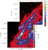 |
Fig. 1 Extinction maps of TMC-1 (southern field, 2MASS data) and TMC-1N (northern field, WFCAM data). |
2.1. WFCAM
We have used the Wide Field CAMera (WFCAM; Casali et al. 2007) of the United Kingdom InfraRed Telescope (UKIRT) to sample a 1° × 1° field in the near-infrared (NIR) J-, H-, and K-bands (1.2, 1.6, and 2.2 μm, respectively) in the Taurus molecular cloud complex field TMC-1N. Our target field choice was based on the Taurus extinction maps of Cambrésy (1999) and Padoan et al. (2002).
We used the ON-OFF method in order to be able to measure diffuse emission. The observations were made during 13 nights between 2006–2008 on 4 × 4 adjacent ON-fields.
The integration times of the ON-fields were 8.5, 11.3, and 27.3 min in the J, H, and K band, respectively. The coordinates of the 4 OFF-fields are (RA (J2000), Dec (J2000)): 3h52m and +23°43′, 3h52m and +24°9′, 3h54m and +23°43′, 3h54m and +24°9′.
The data were reduced in the normal pipeline routine1. In order to study the surface brightness, standard decurtaining methods were needed to remove the stripes caused by the instrument. The reduced data were converted to 2MASS magnitude scale using the formulas of Hewett et al. (2006) and calibrated using 2MASS stars. The Iraf Daophot-package was used for photometry and Montage2 for combining the images. The median magnitudes for which magnitude uncertainty σ ~ 0.1m of our WFCAM data are J = 20.0m, H = 19.1m, and K = 18.8m. These are 4–4.5m deeper than 2MASS observations. In the analysis, we used only sources with σ < 0.1m. Saturated stars were replaced with corresponding 2MASS stars. Based on the classification scheme of Cantiello et al. (2005), potential background galaxies were removed from our star list, in a manner similar to that of Schmalzl et al. (2010).
2.2. 2MASS
We used Two Micron All Sky Survey (2MASS; Skrutskie et al. 2006) data to make extinction maps of the fields for which we did not have deeper observations. We also used 2MASS data for TMC-1N in order to perform a comparison with the WFCAM data that contains a significantly larger number of stars. The sizes of our fields are approximately 1° × 1°. The limiting magnitudes of 2MASS are J = 15.8m, H = 15.1m, and KS = 14.3m.
2.3. Herschel
Both TMC-1 and TMC-1N have also been mapped with Herschel (Pilbratt et al. 2010) as part of the Gould Belt Survey (André et al. 2010). We used SPIRE (Griffin et al. 2010) 250 μm, 350 μm, and 500 μm maps of both of the fields. We obtained the data from the Herschel Gould Belt Survey consortium. The observation identifiers of the data are 1342202252 and 1342202253.
Fields G300.86-9.00 (PCC550) and G163.82-8.44 have been mapped with Herschel as part of the Cold Cores project and are described in more detail in Juvela et al. (2012b).
3. The column density maps
3.1. Column densities from the NIR reddening
The extinction maps were derived from the near-infrared reddening of the background stars, using 2MASS observations for TMC-1 and the WFCAM observations for the northern field TMC-1N. For comparison, an extinction map of TMC-1N was also made using 2MASS data. The extinction values were calculated with the NICER method (Lombardi & Alves 2001), assuming an extinction curve corresponding to RV = 4.0 (Cardelli et al. 1989).
For comparison with the N(H2) values below, the extinction values were converted to N(H2), assuming a relation N(H2) ~ 0.94 × 10²¹ AV (Bohlin et al. 1978). The relation itself is derived for diffuse regions, but serves as a good point of reference for the comparison between the measurements of dust reddening and dust emission. The resolution of the derived column density map is 2′ for 2MASS data and 1′ for WFCAM data.
3.2. Column densities from dust emission
The maps of the dust colour temperature, TC, were calculated
using the SPIRE 250 μm, 350 μm, and
500 μm maps. The data were convolved to a common resolution of 40″ and
the TC values were estimated pixel by pixel assuming a
constant value of the dust spectral index, β = 2.0. The least-squares fit
of modified black body curves
Bν(TC)νβ
provides both the colour temperature and the intensity that were converted to estimates of
column density. The column density was obtained from the formula
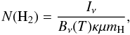 (1)where the dust opacity
per total mass, κ, was assumed to follow the law
0.1 cm2/g (ν/1000 GHz)β that
should be applicable to high density environments (Hildebrand 1983; Beckwith et al. 1990).
The resolution of the column density maps derived from Herschel
observations is 40″.
(1)where the dust opacity
per total mass, κ, was assumed to follow the law
0.1 cm2/g (ν/1000 GHz)β that
should be applicable to high density environments (Hildebrand 1983; Beckwith et al. 1990).
The resolution of the column density maps derived from Herschel
observations is 40″.
4. Modelling the filament profiles
We selected the most prominent filament from each field. The filaments were originally traced by eye and the paths of the filaments were consequently adjusted to follow the crest of the column density as derived from the observations of the dust emission. The filament profiles perpendicular to the filament are extracted at small intervals and the final profile of the filament is obtained by averaging all data along the filament.
We fit the filament column density profiles N(r) with
Plummer-like profiles ![Mathematical equation: \begin{equation} \rho_{p}(r) = \frac{\rho_{\rm c}}{[1+(r/R_{\rm flat})^2]^{p/2}} \Rightarrow N(r) = A_{p} \frac{\rho_{\rm c}R_{\rm flat}}{[1+(r/R_{\rm flat})^2]^{(p-1)/2}} \end{equation}](/articles/aa/full_html/2012/08/aa19573-12/aa19573-12-eq41.png) (2)(see
e.g. Nutter et al. 2008; Arzoumanian et al. 2011). The equation includes the central density
ρc, the size of the flat inner
part Rflat, and the parameter p that
describes the steepness of the profile in the outer parts. We include in the fits two
additional parameters to describe a linear background. According to Ostriker (1964), the value of p should be 4 in the case
of an isothermal cylinder in hydrostatic equilibrium. However, the values that are derived
from observations are often smaller and typically around p ~ 2
(e.g. Arzoumanian et al. 2011; Juvela et al. 2012b). The factor
Ap is obtained from the formula
(2)(see
e.g. Nutter et al. 2008; Arzoumanian et al. 2011). The equation includes the central density
ρc, the size of the flat inner
part Rflat, and the parameter p that
describes the steepness of the profile in the outer parts. We include in the fits two
additional parameters to describe a linear background. According to Ostriker (1964), the value of p should be 4 in the case
of an isothermal cylinder in hydrostatic equilibrium. However, the values that are derived
from observations are often smaller and typically around p ~ 2
(e.g. Arzoumanian et al. 2011; Juvela et al. 2012b). The factor
Ap is obtained from the formula
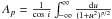 ,
where we assume an inclination angle of i = 0. In addition to the fitted
Plummer profile parameters, we also derive the mass per unit length
Mline of the filament by integrating column density over the
profile.
,
where we assume an inclination angle of i = 0. In addition to the fitted
Plummer profile parameters, we also derive the mass per unit length
Mline of the filament by integrating column density over the
profile.
We use four different methods for extracting the profiles, i.e., profiling. The methods are described in more detail in the following subsections. In short, the profiles are based on a fit to
-
1.
a column density map derived from (submillimetre)dust emission map [Method A];
-
2.
a column density map derived from NIR extinction map [Method B];
-
3.
median AV of stars within a certain offset from the filament centre [Method C];
-
4.
AV of individual stars [Method D].
Method A is currently often used for estimating filament properties. The aim of our study is to investigate, if the alternative methods B, C, and D based on NIR data could also be used for extracting filament profiles.
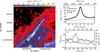 |
Fig. 2 TMC-1N column density map and filament profile derived from WFCAM extinction map. a) Column density map. The part of filament used in the fitting is marked with white line (based on the Herschel column density map in Fig. 3). b) Average column density profile of the filament (black line), fitted Plummer profile (red dashed line) and the baseline of the fit (blue dashed line). Values for fitted Plummer parameters ρc, Rflat, and p are marked in the figure. c) FWHM values (black circles and left hand scale) and column density along the ridge of the filament (solid line and the right hand scale). |
4.1. Extraction of profiles from column density maps
Methods A and B both use a column density map for fitting, but in method A, the column density map is derived from a (submillimetre) dust emission map, and in method B, from a NIR extinction map. Otherwise, the process for extracting the profile parameters is the same. We step along the filament with a step size equal to half of the full width at half maximum (FWHM) of the input map. At each position, we construct the local profile that consists of the values read from the map at intervals of 0.3 × FWHM along a line perpendicular to the filament length. Before averaging, the profiles are aligned in order that their peaks match on the offset axis.
Because the observations have a finite resolution, the data are fitted with a Plummer profile that is convolved to the resolution of the column density map used. Thus, the obtained parameters of the Plummer function should correspond to those of the true filament. In addition to the convolved Plummer profile, we include in the fits a linear background to take into account the possible extended background. The final free parameter is the shift of the Plummer profile that allows for some errors in the position of the originally selected filament. For the dust emission, this already follows the maximum column density. However, it is better to allow a shift in the fit. This applies particularly to the analysis of the extinction where, in principle, the exact position of the observed filament could differ from the position deduced from the dust emission (as is the case in TMC-1, see Figs. 6 and 7).
The estimated FWHM of the filament profile and mass per unit length, Mline, depend on how wide a region is used in the fitting and how the background is removed, as there are no clear limits of where the filaments end, particularly in crowded areas. The fitted Plummer parameters, however, should not depend on the width of the fitting region, as long as the region is wide enough to cover also the edges of the filament. In the fits to the average profile, we only use data where offsets from the filament centre correspond to distances [−0.3 pc, +0.3 pc] for TMC-1 and TMC-1N. For the other filaments shown in Appendix A, we use bigger offset limits, 0.5 pc, in order to make sure that these wider and more distant filaments are properly fitted. We calculate FWHM values for each individual profile and for the median profile after subtracting the minimum. This is directly the observed value without deconvolution with the instrument beam.
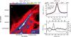 |
Fig. 3 TMC-1N column density map and filament profile derived from Herschel emission map. See Fig. 2 for explanations of the used notation. |
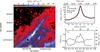 |
Fig. 4 TMC-1N column density map and profile of the densest middle part of the filament derived from WFCAM extinction map. See Fig. 2 for explanations of the used notation. |
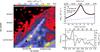 |
Fig. 5 TMC-1N column density map and filament profile derived from 2MASS extinction map. See Fig. 2 for explanations of the used notation. |
4.2. Extraction of profiles using AV of stars directly
The previous extinction maps represent the extinction values of the individual stars that are averaged with a relatively large Gaussian beam. This is necessary in order that no holes remain in the AV map and each pixel value corresponds to the average of at least of a few stars. However, because we are mainly interested in the average properties of the filaments, we can average all the data along the filament length and this should allow us to reach a higher resolution for the profile function. We use two different methods for extracting profiles: median AV values for each offset bin (method C) or direct fit to the AV values of individual stars (method D). In both of these methods we extract profiles only using stars that are within a given offset from the filament centre: [−0.3 pc, +0.3 pc] for TMC-1 and TMC-1N, and [−0.5 pc, +0.5 pc] for the other filaments shown in Appendix A, as in the case of using column density maps.
In method C, we calculate the offset from the filament centre for each star. The stars are binned in narrow offset intervals (i.e., bins extended along the whole filament) and we calculate the median AV for each offset with a step size 0.3 times the bin width. These profiles can again be fitted, taking into account that the binning effectively introduces some loss of resolution. In the following results and simulations, the width of the offset bins is always one arc minute, although we have tested also other values. The drawback of this method is that we cannot use the average and the dispersion of the AV values of the neighbouring stars to filter outliers as effectively. We calculate the FWHM of the median profile after subtracting the minimum. As with column density maps, this is directly the observed value without deconvolution with the instrument beam.
Method D relies directly on the measurements of the individual stars, without any spatial averaging. Each star represents extinction within a very narrow region and the final resolution of the profile function depends only on the density of the stars along the offset axis. The influence of each star is weighted not only according to the uncertainty of its photometry but also inversely proportionally to the local stellar density around the star. Thus, the final profile is weighted according to the area rather than the number of stars within that area. The data are fitted directly with the Plummer profile. Because the individual stars provide a practically infinite resolution, no convolution is needed. In connection with this method we do not calculate any separate FWHM estimates.
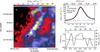 |
Fig. 6 TMC-1 column density map and filament profile derived from 2MASS extinction map (YSOs removed). See Fig. 2 for explanations of the used notation. |
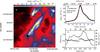 |
Fig. 7 TMC-1 column density map and filament profile derived from Herschel dust emission map. See Fig. 2 for explanations of the used notation. |
5. Results
5.1. Analysis of the column density maps
Column density maps and filament profiles derived from the WFCAM extinction map and Herschel emission map of TMC-1N are shown in Figs. 2 and 3. The filament is traced based on the Herschel map and marked with white line in both column density maps. The filament position obtained from the Herschel map fits very well also in the WFCAM map. In the Herschel map the marked part forms the densest continuous filament, which we call here the full filament. However, in the WFCAM extinction map, the filament continues seamlessly southwards outside the frame.
The profiles obtained by using these two methods (A and B) are very similar. The FWHM of the filament is approximately 0.1 pc, which is in agreement with the general results of Arzoumanian et al. (2011) on filaments in the IC 5146 molecular cloud. When plotting together the column density and FWHM values along the ridge of the filament, we can see a notable anticorrelation between these parameters. In the densest parts of the filament FWHM gets smaller, possibly indicating that gravity is pulling together the mass and forming narrower condensations in the filament, similarly to the results of Juvela et al. (2012b).
The column density structure along the ridge of the filament is quite similar in both data sets. In the Herschel data, the highest peak is narrower and reaches a column density of ~30 × 1021 cm-2 while in the WFCAM data the maximum is ~25 × 1021 cm-2. Considering the many uncertainties in the column density estimates (e.g., dust opacity), the values are practically identical. Conversely, the similarity of the column density values suggests that the assumptions used in the column density calculation were reasonable.
To study the effect of choosing the filament end points, we also extract profiles from the middle part of the filament in TMC-1N, shown in Fig. 4. The average column density is higher than in the full filament. The fitted Plummer parameter values are slightly altered, although the results are quite close to the values obtained using the full filament.
For a comparison using lower resolution data, a column density map and filament profile derived from the 2MASS extinction map of TMC-1N are shown in Fig. 5. Here, the filament position obtained from the Herschel map also fits the filament seen in 2MASS extinction map very well. However, along the filament, the column density peaks are in different positions in maps derived from the Herschel and 2MASS observations. Possible anticorrelation between FWHM and column density along the ridge of the filament is not evident using the 2MASS data. The column density derived from the 2MASS data is notably smaller than the column density derived from the Herschel or WFCAM data. However, we also obtain a similar Plummer profile using 2MASS data.
For a comparison of another filament, column density maps and filament profiles derived from the 2MASS extinction map (YSOs removed) and Herschel emission map of TMC-1 are shown in Figs. 6 and 7. Here the filament is again traced using the Herschel column density map. In this case, the filament position does not exactly match the filament ridge in the 2MASS map. However, this is not a problem in the profiling process, as the filament is allowed to have a small offset from the given position. In this filament, we do not see any notable background gradient or anticorrelation between FWHM and column density along the ridge of the filament. The FWHM of the filament is approximately 0.1–0.2 pc. The column density structure along the ridge differs notably in these two data. In the Herschel data, we see a continuous high density ridge, while in the 2MASS data there is more variation, because of the low number of background stars. Based on the Herschel data, next to the filament there is a distinct clump, which effects the profile and the derived FWHM values. This change in the FWHM values is not seen in the 2MASS data. For a comparison, we show the column density map and filament profiles derived from the 2MASS extinction map before removing YSOs in Fig. B.1.
Obtained parameters describing the filaments TMC-1N (full and middle filament) and TMC-1.
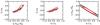 |
Fig. 8 Plummer profile parameter correlations. Contours 1.5
|
The obtained parameters describing the filament, namely FWHM, Plummer parameters and the mass per unit length Mline derived from observations of TMC-1N (full and middle filament) and TMC-1 (before and after removing YSOs) using different methods are shown in Table 1.
We can compare our results for TMC-1 derived from the Herschel maps with those of Nutter et al. (2008), from Submillimetre Common User Bolometer Array (SCUBA; Holland et al. 1999) and the Infrared Space Observatory ISO (Kessler et al. 1996) ISOPHOT instrument (Lemke et al. 1996) data. We note first that we agree on the fact that the Bull’s tail, as they call it, is a filament and not a ring. Both analyses fit Plummer-like profiles, and therefore the results should be comparable (see Table 1). We obtain a value for p of ~2.3, whereas they fix p = 3. We find ρc ~ 7 × 10⁴, compared to their range of ρc ~ 7 × 10⁴ to ~1.7 × 10⁵ (with nominal values towards the upper end of this range). Our value for Rflat is ~0.04 pc, and their value is ~0.05 pc. We find the FWHM to be 0.12 pc for the Herschel data, and ~0.18 pc for the 2MASS data. They fitted the filament with two components, the first of which had a FWHM of 0.11 pc and the second of which had a FWHM of 0.16 pc. It can therefore be seen that there is a high degree of consistency, giving us added confidence in our parameter fitting of the data.
The WFCAM AV maps and Herschel column density maps give very similar results for the FWHM of the TMC-1N filament (0.092 and 0.093 pc, respectively). Lower resolution AV maps based on 2MASS stars give slightly higher values for FWHM (0.17 pc). The behaviour of the Plummer parameters or Mline derived from these is not as predictable, as there are dependencies between the parameters. We examine these dependencies more closely below. In addition, the exact values seem to be quite sensitive for instance to small changes in the data, different resolution data, fitting algorithm, initial fitting parameter values or different profiling method. We also noticed that the chosen pixel size for the extinction maps can alter the results.
In order to study the correlations of the Plummer profile parameters we save
cross-sections of χ2. We fix each of the
parameters ρc, Rflat or
p in turn to the fitted value, and change the others systematically to
extract the χ2 values in three orthogonal parameter planes
crossing at the location of
the χ2 minimum,  . In
Fig. 8, we show the contour levels 1.5
and 10
, for each
case. The results show that there is a banana shaped correlation
between Rflat and p, more or less linear
(in log-space) correlation between ρc and p,
and a linear anticorrelation between ρc
and Rflat. Even the 1.5
contours are
quite wide, especially in
ρc–Rflat-plane, meaning that very
different parameter values can give small χ2 values. There are
also differences in the size and orientation of the contours when comparing
Herschel emission maps and WFCAM extinction maps. The
1.5 contours are
smaller when using WFCAM extinction map
in Rflat–p-plane and
ρc–p-plane. However, in
ρc–Rflat-plane the contours are
smaller when using Herschel emission maps.
. In
Fig. 8, we show the contour levels 1.5
and 10
, for each
case. The results show that there is a banana shaped correlation
between Rflat and p, more or less linear
(in log-space) correlation between ρc and p,
and a linear anticorrelation between ρc
and Rflat. Even the 1.5
contours are
quite wide, especially in
ρc–Rflat-plane, meaning that very
different parameter values can give small χ2 values. There are
also differences in the size and orientation of the contours when comparing
Herschel emission maps and WFCAM extinction maps. The
1.5 contours are
smaller when using WFCAM extinction map
in Rflat–p-plane and
ρc–p-plane. However, in
ρc–Rflat-plane the contours are
smaller when using Herschel emission maps.
5.2. Profiles using AV of stars directly
Profiles of TMC-1N full filament derived by using methods C and D with WFCAM data and 2MASS data are shown in Fig. 9. The profile of TMC-1N middle filament using the WFCAM data is shown in Fig. 10, and the profile of TMC-1 using the 2MASS data is shown in Fig. 11. The obtained parameters derived from observations of TMC-1N (full and middle filament, WFCAM and 2MASS data) and TMC-1 (2MASS data) are shown in Table 1. The results of using median averages (method C) are on the “Median profile” and the results of using individual stars (method D) on the “Fit to individual stars” line. The results obtained for TMC-1 before and after removing the YSOs were identical when using methods C and D.
The values obtained with methods C and D are quite similar to the values derived from maps. However, as with the map method, the derived parameters are quite sensitive to small changes in the data. For example, for the TMC-1N full filament using the WFCAM data, the star methods give notably larger values for p than the map methods, but when only the densest middle part of the filament is profiled, these differences get smaller.
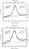 |
Fig. 9 Profiles of TMC-1N filament derived by using methods C and D in WFCAM data (top frame) and 2MASS data (bottom frame). Blue stars: median values. Grey line: Plummer profile before convolution, fitted to the median AV values of stars. Black solid line: the convolved Plummer profile. Red solid line: fit to individual stars (not marked in the picture). Dashed lines: fitted linear baselines for Plummer fits shown with the same colours. |
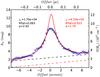 |
Fig. 10 Profile of TMC-1N middle filament derived by using individual stars or their median averages in WFCAM data. See Fig. 9 for explanations of the used notation. |
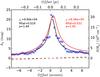 |
Fig. 11 Profiles of TMC-1 filament derived by using individual stars or their median averages in 2MASS data. See Fig. 9 for explanations of the used notation. |
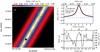 |
Fig. 12 Example of a simulated map and filament profile without noise. Used parameter values in the simulation: ρc = 104 cm-3, Rflat = 0.025, p = 2.0, stellar density =1.0, and without photometric noise. The fitted parameter values are shown in frame b). See Fig. 2 for explanations of the used notation. |
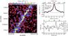 |
Fig. 13 Example of a simulated map and filament profile with noise. Used parameter values: ρc = 104 cm-3, Rflat = 0.025, p = 2.0, stellar density =1.0, and noise =1.0 (meaning a similar noise level as in our WFCAM observations of TMC-1N.). The fitted parameter values are shown in frame b). See Fig. 2 for explanations of the used notation. |
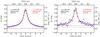 |
Fig. 14 Examples of simulated profiles using methods C and D. Used parameter values: ρc = 104 cm-3, Rflat = 0.025, p = 2.0, stellar density =1.0, and without noise (left frame) or with noise (right frame). The fitted parameter values are shown in the figure. See Fig. 9 for explanations of the used notation. |
6. Simulated extinction observations
We use simulations to examine the accuracy with which the filament profiles can be estimated from the observations of background stars. As a reference, we use the WFCAM observations from which we estimate the probability distribution of the number of stars as a function of the H-band magnitude, the average J − H and H − K colours, and the uncertainties of these colours as a function of the magnitude. These data are used in simulations in which we place background stars at random positions over an area of 30′ × 30′. As a reference, we use the stellar density in the WFCAM observations but also test the effect of lower and higher stellar densities. The stellar colours are reddened according to the column density distribution that results from the presence of a filament. The density distribution of the filament follows the Plummer function with chosen parameters. The filament is assumed to be in the plane of the sky but has a position angle of 30° in order to avoid the special case where the filament would be aligned with the axes used in the pixelisation of the extinction maps.
The extinctions of the individual stars (and of the 30′ × 30′ extinction map) are calculated using one corner (78 square arc minutes) of the simulated region as a reference area from which the intrinsic stellar colours are estimated. The simulated observations are then analysed as in the case of the WFCAM observations above. The filament parameters are derived from the extinction map (method B), from the median profile along the filament (method C), and from the direct fit of the Plummer profile to the AV values of the individual stars (method D). We analyse a 20′ long part of the filament that thus fits well within the 30′ × 30′ area with the assumed distance of 140 pc, even taking into account the non-zero position angle.
In the simulations, Rflat is always 0.025, and there is no background gradient. We compare our three methods and the way the fitted p, ρc and derived Mline change when we use different sets of parameter values for ρc (104, 105, 106 cm-3), p (2, 3, 4), and stellar density (0.2, 0.5, 1, 2, 5, 10, where 1 denotes the stellar density in the WFCAM observations). We also test how photometric noise affects the results by using different noise levels 0, 0.3, and 1, where 1 denotes the photometric noise level in the WFCAM observations of TMC-1N. Even when the photometric noise is zero, there is still noise in the data, because the stars have a random position and brightness, i.e., some stars may be extincted below the detection threshold. The filament looks different depending on the number and brightness of the stars situated in the filament area. The filament is well defined, if there are enough bright stars near the borders of the filament, where they can still be seen. We run each simulation case 100 times for the estimation of the uncertainties.
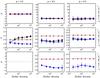 |
Fig. 15 Plummer p parameter derived from simulated extinction observations without noise. Different central densities are shown on different lines: 104 (cm-3) (uppermost frames), 105 (middle frames), and 106 (bottom frames). Symbols and colours denote the used method: method B (black square), method C (blue circle), and method D (red star). Stellar density is given on the x-axis, where 1 means a similar density as in the WFCAM observations of TMC-1N. The true p value (2, 3 or 4) used in the simulations is given on top of each column and also shown as a dashed line in the figures. The derived p value is marked in the figures for each simulated stellar density and method with scale on the y-axis. |
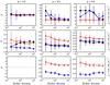 |
Fig. 16 Plummer p parameter derived from simulated extinction observations with noise =1 (times WFCAM noise). See Fig. 15 for explanations of the used notation. |
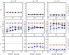 |
Fig. 17 Plummer ρc parameter derived from simulated extinction observations without noise. Y-axis denoting the fitted ρc is divided with the correct ρc. See Fig. 15 for explanations of the used notation. |
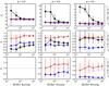 |
Fig. 18 Plummer ρc parameter derived from simulated extinction observations with noise =1. See Figs. 15 and 17 for explanations of the used notation. |
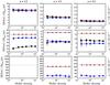 |
Fig. 19 Mline derived from simulated extinction observations with noise =0. The true Mline is marked with a dashed line in the figures. The derived Mline is marked in the figures for each simulated stellar density and method with scale on the y-axis. Otherwise, see Fig. 15 for explanations of the used notation. |
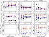 |
Fig. 20 Mline derived from simulated extinction observations with noise =1. See Figs. 15 and 19 for explanations of the used notation. |
6.1. Simulation results
Examples of simulated maps and filament profiles with and without photometric noise are shown in Figs. 12 and 13. The simulated profiles of the same cases using methods C and D are shown in Fig. 14. The resulting column density maps resemble our TMC-1N observations, except that the density distribution precisely follows the Plummer function with a chosen set of parameters. If all the simulated filaments are examined along their whole length, there is no clear anti-correlation (nor correlation) between observed FWHM and column density along the ridge. However, similarly to the observations of TMC-1N (Fig. 2, frame c), anticorrelation can sometimes be seen in some of the densest peaks also in simulations, even though the simulated filament itself is symmetric.
The filament parameters are derived from the simulated observations. In Figs. 15–20, we compare the true and estimated parameter values p, ρc, and Mline for cases with different parameter values and different number of background stars. The error bars correspond to half of the interquartile range between the 75% and 25% percentiles.
Figure 15 shows that in a noiseless situation method D works almost perfectly in fitting the p parameter. The error bars of method D are not visible in the figure, because they are so small. This is natural as the random positions of the stars do not affect this method and the photometry itself does not contain errors. Methods B and C also work well for modest density, ρc = 104 cm-3, being correct to within 10%. However, in higher density (ρc = 105 cm-3) both of these methods underestimate the p value, except in the case p = 2, where method B ends up overestimating the p value. Still, both methods are correct to within 20%. Method B does not work reliably at densities as high as 106 cm-3, because stars cannot be seen at the centre of the filament. It is therefore left out of the figures. The case of density 106 cm-3 and p = 2 is not shown either with methods C and D, as the results get unreliable when the empty part in the middle is too wide. However, with larger p values both methods C and D continue to work also at high densities, although method C underestimates the p value ~20%. We also made some tests with density 103 cm-3, but for such low density the filament is no longer reliably identified. The combination of central density and true parameter p determines how well the observed parameter p is fitted.
The results with photometric noise similar to WFCAM observations are shown in Fig. 16. The results are still similar to those without noise, except that the errors get larger. For density 104 cm-3 and parameter p = 2.0 the bias is very small with all star densities and all methods, but in the case of very low star density (0.2), the scatter for method C is so large that the method does not work reliably. For density 104 cm-3 and parameter p = 4.0, both methods B and C typically result in a value of p = 10, the maximum allowed in the fitting procedure. This means that in these cases the results of the fits are not reliable. Still, in most cases the results are correct to within 10% for method D and to within 20% for the other methods.
Figures 17 and 18 show, that ρc is also fitted quite reliably, especially using methods D and C for modest (ρc ~ 104 cm-3) densities and without photometric noise. If noise is included, method B tends to overestimate the density for the modest density case, especially when the star density is low. For higher densities (ρc > = 105 cm-3), both methods B and C underestimate the density, even though the results are still correct to within an order of magnitude. The derived Mline shows a similar behaviour in Figs. 19 and 20. Method D gives correct results to within 10% in most cases. Methods B and C also give correct results to within 10% for modest density (ρc ~ 104 cm-3). For higher densities, methods B and C both underestimate the mass by ~20% or even up to ~60% in the densest case.
Generally, all the compared methods seem to produce reliable results in most cases, especially with modest density (104 cm-3). In addition, when stellar density grows, the errors become smaller. For higher densities, method D usually seems to give the most reliable value.
7. Discussion
The characteristics of interstellar filament properties are currently approached using mainly submillimetre studies, due to the high resolution data obtained with Herschel. However, if such data are not available, the use of groundbased NIR data would be more convenient. We have therefore compared the profiles obtained from column density maps derived from both submillimetre dust emission maps (method A) and NIR extinction maps (method B).
We have presented two new methods to derive filament profiles. In method C we divide the stars to bins according to their distance from the filament centre, calculate the median AV for each offset bin and fit a Plummer profile to the median AV values. In method D we fit the Plummer profiles directly to the AV values of individual stars, without any spatial averaging.
The results of the profile fits to TMC-1N and TMC-1 (Table 1) show, that all four methods give rather similar results. Of course, with observations we do not know which values are the most correct ones. There does not seem to be any obvious systematic biases in different methods, e.g., AV maps can sometimes give a lower (in TMC-1) and sometimes higher (in TMC-1N) values for masses than the Herschel emission maps. In general, the fitted densities are similar to within an order of magnitude. The fitted p values change relatively much, between 1.67–4.57 for TMC-1N (full filament), 1.56–3.38 for TMC-1N (middle filament), and 1.84–3.60 for TMC-1, depending of the method. However, in the other two filaments shown in Appendix A, the p values are much more stable (1.92–2.1 and 1.31–1.79).
YSOs embedded in the filaments could bias the extinction estimates, as they are redder than background stars. Even the effect of a single YSO could be notable in dense filaments, if only a few stars are seen in the middle of the filament. There are six known YSOs in the TMC-1 filament area used in our profiles. We have tested the effect of YSOs in this filament, and note that removing the YSOs can have significant local effects in the column density maps and profiles along the ridge of the filament. However, in this case, the profile parameters derived with or without YSOs stay identical when using methods C or D. Using method B, there is some change in the fits, but the parameter values are still similar to within ~10–30%.
We have noticed that the Plummer profile fits are quite sensitive to small changes in the data or the fitting routines. The dependencies of the Plummer parameters in Fig. 8 show that the confidence regions of Plummer parameters are quite wide. This confirms our findings, that the parameters are not always well constrained and therefore small changes in the data can lead to different parameter values. The correlations of the parameters, e.g. Rflat and p, should therefore be taken into account, instead of giving too much weight on the value of a single parameter. The emission and extinction data are independent and together should result in more accurate estimates of the filament parameters. This is particularly true when the orientations of the corresponding confidence regions (i.e., the minimum χ2 contours) are different.
We have used simulations to compare the filament parameters and the derived mass per unit length Mline obtained with extinction maps and the two alternative methods. We have tested the limit of the methods using different densities ρc (104, 105, 106 cm-3) and stellar densities (0.2, 0.5, 1, 2, 5, 10, where 1 denotes the stellar density in the WFCAM observations). Tests with ρc = 103 showed, that in these low densities the extinction methods did not work reliably. The simulations show that method D gives correct results to within 10% in most cases. Methods B and C also work in most cases correctly to within ~20%. Only for high densities (106 cm-3) can the bias for method C be notably larger, and method B cannot reliably be used. When using method D in high density the scatter can grow so much that the results are unreliable, even though the bias can still be small. When stellar density grows, the results become more accurate. However, the simulations showed that all the methods also work in most cases with stellar densities below that of our WFCAM observations.
In nearby, high galactic latitude clouds, such as Taurus, foreground stars do not cause a problem in the analysis. In other cases, however, foreground stars could cause a notable bias. We have examined the effect of foreground stars in simulations. Changing ~10% of the background stars to foreground stars can cause ~10–30% more bias in the mass estimates. The method D is quite robust when no noise is included, but the difference to the other methods is diminished, when realistic noise is added.
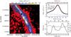 |
Fig. A.1 G300.86-9.00 (PCC550) column density map and filament profile derived from 2MASS extinction map. See Fig. 2 for explanations of the used notation. |
The key question is, what kind of conclusions can be made of the observations on the basis of simulations. In the WFCAM observations of TMC-1N, the value of central density is estimated to be between 104–105 cm-3, which is within the range of our simulations. In this case, in particular method D should be quite reliable according to our simulations (see Figs. 16 and 20). However, the simulations are simplifications of true filaments, and they do not take into account all factors that could affect the interpretations. For example, there is no background gradient in the simulations, whereas in the observed area, there is a strong gradient that could distort the obtained parameters. A linear background is included as a free parameter in the fitting of Plummer profile, and therefore a linear background gradient perpendicular to the filament should not cause problems. However, nonlinear gradients could affect the fitting. In the simulations the filament is also assumed to be in the plane of the sky. All the generated photometric errors are normally distributed. In real observations, there could be outliers, which could affect both methods C and D.
However, the fundamental question is, whether or not the real filament profiles are really Plummer functions. In the simulations, we presume that the filament profile obeys the Plummer function, and therefore the results fit well that function unless there is some bias. In real observations, this is not necessarily the case. We have also noticed that even a poor fit can give reasonable values for the Plummer parameters. Conversely, good fits can also give, e.g., very high values for the p parameter. It is therefore advisable that all fits are checked by eye, even for large surveys.
The methods could be further improved, e.g., by carrying out a separate outlier filtering step (on AV map) before using method D, or weighting the profiles according to the number of stars in the median bins in method C. Background structure could also be modelled and subtracted before extracting the profiles. In principle, a linear background should not affect the resulting profiles, but in practise the fits seemed to be quite sensitive to any small variations in the data.
We have shown that filament profiles can be derived from NIR extinction data. These methods can serve as a valuable point of comparison to the results obtained with Herschel or other instruments using submillimetre dust emission. The methods can be used with, e.g., UKIDSS and future NIR surveys, but we have also shown that even 2MASS data can give rather reliable estimates in the case of very nearby clouds. NIR extinction and groundbased dust emission measurements with, e.g., SCUBA-II can be used as alternative or complementary means of studying the properties of filaments. The limits of the NIR extinction methods come from the requirements of having enough background stars. This restricts the use of these methods to low latitudes and nearby sources. The resolution of the method is limited only by the amount of background stars.
In order to achieve better resolution, NIR surface brightness could be used (see e.g. Padoan et al. 2006; Juvela et al. 2006, 2008). However, the observations of NIR surface brightness can be quite difficult. We study the properties of TMC-1N using NIR surface brightness data in a following paper (Malinen et al., in prep.).
8. Conclusions
We have compared the filament profiles obtained by submillimetre observations (method A) and NIR extinction (methods B, C, and D).
-
We conclude that NIR extinction maps(method B) can be used as an alternative method to submillimetre observations to profile molecular cloud filaments.
-
We show that if better resolution NIR data are not available, 2MASS data can also be used to estimate approximate profiles of nearby filaments.
-
We also present two new methods for the derivation of filament profiles using NIR extinction data:
-
Plummer profile fits to medianAV values of stars within certain offset bin from the filament centre (method C)
-
Plummer profile fits directly to the AV values of individual stars (method D)
-
-
We show that in simulations, all the methods based on NIR extinction work best with modest densities ρc = 104–105 cm-3. Method D gives correct results for the fitted and derived parameters to within ~10% and methods B and C to within ~20% in most cases. At high densities (~106 cm-3), only method D continues to work reliably.
-
For the profile fits to real observations the values of individual Plummer parameters are in general similar to within a factor of ~2 (in some cases up to a factor of ~5). Although the Plummer parameter values can show significant variation, the derived estimates of filament mass (per unit length) usually remain accurate to within some tens of per cent.
-
We confirm the earlier results of Nutter et al. (2008) that the examined TMC-1 structure, or Bull’s tail, is a filament and not part of a continuous ring. Our parameter values are also consistent with the earlier results.
-
The confidence regions of the Plummer parameters are quite wide. As the parameters are not always well constrained, even small changes in the data can lead to different parameter values. The correlations of the parameters should therefore be taken into account.
-
The size and orientation of the confidence regions are not identical when Herschel maps or NIR data are used. The combination of the methods can significantly improve the accuracy of the filament parameter estimates.
http://montage.ipac.caltech.edu/
Acknowledgments
We thank the referee, Laurent Cambrésy, for suggestions that improved the paper. We are grateful to Mike Irwin for reducing the WFCAM data. J.M. and M.J. acknowledge the support of the Academy of Finland Grants Nso. 250741 and 127015. J.M. also acknowledges a grant from Magnus Ehrnrooth Foundation. M.G.R. gratefully acknowledges support from the Joint ALMA Observatory and the Joint Astronomy Centre, Hawaii (UKIRT). P.P. is funded by the Fundação para a Ciência e a Tecnologia (Portugal). The United Kingdom Infrared Telescope is operated by the Joint Astronomy Centre on behalf of the Science and Technology Facilities Council of the UK. This paper makes use of WFCAM observations processed by the Cambridge Astronomy Survey Unit (CASU) at the Institute of Astronomy, University of Cambridge. This publication makes use of data products from the Two Micron All Sky Survey, which is a joint project of the University of Massachusetts and the Infrared Processing and Analysis Center/California Institute of Technology, funded by the National Aeronautics and Space Administration and the National Science Foundation. This research made use of Montage, funded by the National Aeronautics and Space Administration’s Earth Science Technology Office, Computation Technologies Project, under Cooperative Agreement Number NCC5-626 between NASA and the California Institute of Technology. Montage is maintained by the NASA/IPAC Infrared Science Archive.
References
- André, P., Men’shchikov, A., Bontemps, S., et al. 2010, A&A, 518, L102 [NASA ADS] [CrossRef] [EDP Sciences] [Google Scholar]
- Arzoumanian, D., André, P., Didelon, P., et al. 2011, A&A, 529, L6 [Google Scholar]
- Beckwith, S. V. W., Sargent, A. I., Chini, R. S., & Guesten, R. 1990, AJ, 99, 924 [NASA ADS] [CrossRef] [Google Scholar]
- Bohlin, R. C., Savage, B. D., & Drake, J. F. 1978, ApJ, 224, 132 [NASA ADS] [CrossRef] [Google Scholar]
- Cambrésy, L. 1999, A&A, 345, 965 [NASA ADS] [Google Scholar]
- Cantiello, M., Blakeslee, J. P., Raimondo, G., et al. 2005, ApJ, 634, 239 [NASA ADS] [CrossRef] [Google Scholar]
- Cardelli, J. A., Clayton, G. C., & Mathis, J. S. 1989, ApJ, 345, 245 [NASA ADS] [CrossRef] [Google Scholar]
- Casali, M., Adamson, A., Alves de Oliveira, C., et al. 2007, A&A, 467, 777 [NASA ADS] [CrossRef] [EDP Sciences] [Google Scholar]
- Goodman, A. A., Pineda, J. E., & Schnee, S. L. 2009, ApJ, 692, 91 [NASA ADS] [CrossRef] [Google Scholar]
- Griffin, M. J., Abergel, A., Abreu, A., et al. 2010, A&A, 518, L3 [Google Scholar]
- Hewett, P. C., Warren, S. J., Leggett, S. K., & Hodgkin, S. T. 2006, MNRAS, 367, 454 [NASA ADS] [CrossRef] [Google Scholar]
- Hildebrand, R. H. 1983, QJRAS, 24, 267 [NASA ADS] [Google Scholar]
- Hill, T., Motte, F., Didelon, P., et al. 2011, A&A, 533, A94 [NASA ADS] [CrossRef] [EDP Sciences] [Google Scholar]
- Holland, W. S., Robson, E. I., Gear, W. K., et al. 1999, MNRAS, 303, 659 [NASA ADS] [CrossRef] [MathSciNet] [Google Scholar]
- Juvela, M., Pelkonen, V.-M., Padoan, P., & Mattila, K. 2006, A&A, 457, 877 [NASA ADS] [CrossRef] [EDP Sciences] [Google Scholar]
- Juvela, M., Pelkonen, V.-M., Padoan, P., & Mattila, K. 2008, A&A, 480, 445 [NASA ADS] [CrossRef] [EDP Sciences] [Google Scholar]
- Juvela, M., Malinen, J., & Lunttila, T. 2012a, A&A, in press, DOI: 10.1051/0004-6361/201219558 [Google Scholar]
- Juvela, M., Ristorcelli, I., Pagani, L., et al. 2012b, A&A, 541, A12 [NASA ADS] [CrossRef] [EDP Sciences] [Google Scholar]
- Kessler, M. F., Steinz, J. A., Anderegg, M. E., et al. 1996, A&A, 315, L27 [NASA ADS] [Google Scholar]
- Kirk, J. M., Ward-Thompson, D., Palmeirim, P., et al. 2012, MNRAS, submitted [Google Scholar]
- Lemke, D., Klaas, U., Abolins, J., et al. 1996, A&A, 315, L64 [NASA ADS] [Google Scholar]
- Lombardi, M., & Alves, J. 2001, A&A, 377, 1023 [NASA ADS] [CrossRef] [EDP Sciences] [Google Scholar]
- Lombardi, M., Lada, C. J., & Alves, J. 2010, A&A, 512, A67 [NASA ADS] [CrossRef] [EDP Sciences] [Google Scholar]
- Malinen, J., Juvela, M., Collins, D. C., Lunttila, T., & Padoan, P. 2011, A&A, 530, A101 [NASA ADS] [CrossRef] [EDP Sciences] [Google Scholar]
- Nutter, D., Kirk, J. M., Stamatellos, D., & Ward-Thompson, D. 2008, MNRAS, 384, 755 [NASA ADS] [CrossRef] [Google Scholar]
- Ostriker, J. 1964, ApJ, 140, 1056 [NASA ADS] [CrossRef] [MathSciNet] [Google Scholar]
- Padoan, P., Juvela, M., Goodman, A. A., & Nordlund, Å. 2001, ApJ, 553, 227 [NASA ADS] [CrossRef] [Google Scholar]
- Padoan, P., Cambrésy, L., & Langer, W. 2002, ApJ, 580, L57 [NASA ADS] [CrossRef] [Google Scholar]
- Padoan, P., Juvela, M., & Pelkonen, V.-M. 2006, ApJ, 636, L101 [NASA ADS] [CrossRef] [Google Scholar]
- Pilbratt, G. L., Riedinger, J. R., Passvogel, T., et al. 2010, A&A, 518, L1 [CrossRef] [EDP Sciences] [Google Scholar]
- Rebull, L. M., Koenig, X. P., Padgett, D. L., et al. 2011, ApJS, 196, 4 [NASA ADS] [CrossRef] [Google Scholar]
- Schmalzl, M., Kainulainen, J., Quanz, S. P., et al. 2010, ApJ, 725, 1327 [NASA ADS] [CrossRef] [Google Scholar]
- Ward-Thompson, D., Di Francesco, J., Hatchell, J., et al. 2007, PASP, 119, 855 [NASA ADS] [CrossRef] [Google Scholar]
Appendix A: Comparing filament profiling in Herschel fields and 2MASS data
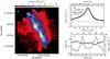 |
Fig. A.2 300.86-9.00 (PCC550) column density map and filament profile derived from Herschel emission map. See Fig. 2 for explanations of the used notation. |
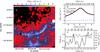 |
Fig. A.3 G163.82-8.44 column density map and filament profile derived from 2MASS extinction map. See Fig. 2 for explanations of the used notation. |
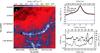 |
Fig. A.4 G163.82-8.44 column density map and filament profile derived from Herschel emission map. See Fig. 2 for explanations of the used notation. |
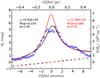 |
Fig. A.5 Profiles of 300.86-9.00 (PCC550) filament derived by using methods C and D on 2MASS data. See Fig. 9 for explanations of the used notation. |
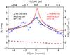 |
Fig. A.6 Profiles of G163.82-8.44 filament derived by using methods C and D on 2MASS data. See Fig. 9 for explanations of the used notation. |
Obtained parameters describing the filaments G300.86-9.00 and G163.82-8.44.
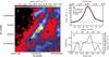 |
Fig. B.1 TMC-1 column density map and filament profile derived from 2MASS extinction map (YSOs not removed). See Fig. 2 for explanations of the used notation. See Fig. 6 for a map and profiles derived after the YSOs are removed. |
We compare our methods to two profiles obtained using Herschel column density maps presented in Juvela et al. (2012b), namely fields G300.86-9.00 (PCC550) and G163.82-8.44. The distances to these filaments are ~230 pc and 350 pc, respectively. Column density maps and filament profiles derived from 2MASS extinction maps and Herschel emission maps are shown in Figs. A.1 and A.2 for G300.86-9.00, and A.3 and A.4 for G163.82-8.44.
The filaments are traced based on the Herschel maps and marked with white line in both column density maps. The filament positions obtained from Herschel maps fit quite well also in the 2MASS maps. Profiles of the filaments derived by methods C and D using 2MASS data are shown in Figs. A.5 and A.6. The filament parameters derived with different methods are shown in Table A.1. The differences to the results of Juvela et al. (2012b) are caused by small modifications in the method and the change of the selected filament segment. The distance to these filaments is greater than to TMC-1, which means that there are fewer stars in the filament area and a larger probability of foreground stars, which can bias the results. However, in general, we obtain quite similar results using all our four methods. In these filaments anticorrelation of FWHM in the densest peaks is also quite clear in the Herschel maps, but not in the 2MASS maps.
Appendix B: Effects of YSOs
YSOs may bias the extinction estimates, if they are not removed. For a comparison to Fig. 6 made after removing the YSOs (six in the profiled filament area), we show in Fig. B.1 the column density map and profiles of TMC-1 made before removing the YSOs. Even though the derived profile parameter values for both cases are similar to within ~10–30%, notable local changes can occur in the column density maps and in the column density profiles along the ridge of the filament.
All Tables
Obtained parameters describing the filaments TMC-1N (full and middle filament) and TMC-1.
All Figures
|
Fig. 1 Extinction maps of TMC-1 (southern field, 2MASS data) and TMC-1N (northern field, WFCAM data). |
| In the text | |
|
Fig. 2 TMC-1N column density map and filament profile derived from WFCAM extinction map. a) Column density map. The part of filament used in the fitting is marked with white line (based on the Herschel column density map in Fig. 3). b) Average column density profile of the filament (black line), fitted Plummer profile (red dashed line) and the baseline of the fit (blue dashed line). Values for fitted Plummer parameters ρc, Rflat, and p are marked in the figure. c) FWHM values (black circles and left hand scale) and column density along the ridge of the filament (solid line and the right hand scale). |
| In the text | |
|
Fig. 3 TMC-1N column density map and filament profile derived from Herschel emission map. See Fig. 2 for explanations of the used notation. |
| In the text | |
|
Fig. 4 TMC-1N column density map and profile of the densest middle part of the filament derived from WFCAM extinction map. See Fig. 2 for explanations of the used notation. |
| In the text | |
|
Fig. 5 TMC-1N column density map and filament profile derived from 2MASS extinction map. See Fig. 2 for explanations of the used notation. |
| In the text | |
|
Fig. 6 TMC-1 column density map and filament profile derived from 2MASS extinction map (YSOs removed). See Fig. 2 for explanations of the used notation. |
| In the text | |
|
Fig. 7 TMC-1 column density map and filament profile derived from Herschel dust emission map. See Fig. 2 for explanations of the used notation. |
| In the text | |
|
Fig. 8 Plummer profile parameter correlations. Contours 1.5
|
| In the text | |
|
Fig. 9 Profiles of TMC-1N filament derived by using methods C and D in WFCAM data (top frame) and 2MASS data (bottom frame). Blue stars: median values. Grey line: Plummer profile before convolution, fitted to the median AV values of stars. Black solid line: the convolved Plummer profile. Red solid line: fit to individual stars (not marked in the picture). Dashed lines: fitted linear baselines for Plummer fits shown with the same colours. |
| In the text | |
|
Fig. 10 Profile of TMC-1N middle filament derived by using individual stars or their median averages in WFCAM data. See Fig. 9 for explanations of the used notation. |
| In the text | |
|
Fig. 11 Profiles of TMC-1 filament derived by using individual stars or their median averages in 2MASS data. See Fig. 9 for explanations of the used notation. |
| In the text | |
|
Fig. 12 Example of a simulated map and filament profile without noise. Used parameter values in the simulation: ρc = 104 cm-3, Rflat = 0.025, p = 2.0, stellar density =1.0, and without photometric noise. The fitted parameter values are shown in frame b). See Fig. 2 for explanations of the used notation. |
| In the text | |
|
Fig. 13 Example of a simulated map and filament profile with noise. Used parameter values: ρc = 104 cm-3, Rflat = 0.025, p = 2.0, stellar density =1.0, and noise =1.0 (meaning a similar noise level as in our WFCAM observations of TMC-1N.). The fitted parameter values are shown in frame b). See Fig. 2 for explanations of the used notation. |
| In the text | |
|
Fig. 14 Examples of simulated profiles using methods C and D. Used parameter values: ρc = 104 cm-3, Rflat = 0.025, p = 2.0, stellar density =1.0, and without noise (left frame) or with noise (right frame). The fitted parameter values are shown in the figure. See Fig. 9 for explanations of the used notation. |
| In the text | |
|
Fig. 15 Plummer p parameter derived from simulated extinction observations without noise. Different central densities are shown on different lines: 104 (cm-3) (uppermost frames), 105 (middle frames), and 106 (bottom frames). Symbols and colours denote the used method: method B (black square), method C (blue circle), and method D (red star). Stellar density is given on the x-axis, where 1 means a similar density as in the WFCAM observations of TMC-1N. The true p value (2, 3 or 4) used in the simulations is given on top of each column and also shown as a dashed line in the figures. The derived p value is marked in the figures for each simulated stellar density and method with scale on the y-axis. |
| In the text | |
|
Fig. 16 Plummer p parameter derived from simulated extinction observations with noise =1 (times WFCAM noise). See Fig. 15 for explanations of the used notation. |
| In the text | |
|
Fig. 17 Plummer ρc parameter derived from simulated extinction observations without noise. Y-axis denoting the fitted ρc is divided with the correct ρc. See Fig. 15 for explanations of the used notation. |
| In the text | |
|
Fig. 18 Plummer ρc parameter derived from simulated extinction observations with noise =1. See Figs. 15 and 17 for explanations of the used notation. |
| In the text | |
|
Fig. 19 Mline derived from simulated extinction observations with noise =0. The true Mline is marked with a dashed line in the figures. The derived Mline is marked in the figures for each simulated stellar density and method with scale on the y-axis. Otherwise, see Fig. 15 for explanations of the used notation. |
| In the text | |
|
Fig. 20 Mline derived from simulated extinction observations with noise =1. See Figs. 15 and 19 for explanations of the used notation. |
| In the text | |
|
Fig. A.1 G300.86-9.00 (PCC550) column density map and filament profile derived from 2MASS extinction map. See Fig. 2 for explanations of the used notation. |
| In the text | |
|
Fig. A.2 300.86-9.00 (PCC550) column density map and filament profile derived from Herschel emission map. See Fig. 2 for explanations of the used notation. |
| In the text | |
|
Fig. A.3 G163.82-8.44 column density map and filament profile derived from 2MASS extinction map. See Fig. 2 for explanations of the used notation. |
| In the text | |
|
Fig. A.4 G163.82-8.44 column density map and filament profile derived from Herschel emission map. See Fig. 2 for explanations of the used notation. |
| In the text | |
|
Fig. A.5 Profiles of 300.86-9.00 (PCC550) filament derived by using methods C and D on 2MASS data. See Fig. 9 for explanations of the used notation. |
| In the text | |
|
Fig. A.6 Profiles of G163.82-8.44 filament derived by using methods C and D on 2MASS data. See Fig. 9 for explanations of the used notation. |
| In the text | |
|
Fig. B.1 TMC-1 column density map and filament profile derived from 2MASS extinction map (YSOs not removed). See Fig. 2 for explanations of the used notation. See Fig. 6 for a map and profiles derived after the YSOs are removed. |
| In the text | |
Current usage metrics show cumulative count of Article Views (full-text article views including HTML views, PDF and ePub downloads, according to the available data) and Abstracts Views on Vision4Press platform.
Data correspond to usage on the plateform after 2015. The current usage metrics is available 48-96 hours after online publication and is updated daily on week days.
Initial download of the metrics may take a while.