| Issue |
A&A
Volume 544, August 2012
|
|
|---|---|---|
| Article Number | A111 | |
| Number of page(s) | 16 | |
| Section | Galactic structure, stellar clusters and populations | |
| DOI | https://doi.org/10.1051/0004-6361/201219314 | |
| Published online | 08 August 2012 | |
The mass function of the Coma Berenices open cluster below 0.2 M⊙: a search for low-mass stellar and substellar members⋆
1 Thüringer Landessternwarte Tautenburg, Sternwarte 5, 07778 Tautenburg, Germany
e-mail: This email address is being protected from spambots. You need JavaScript enabled to view it.
2 Ulugh Beg Astronomical Institute, Astronomical str. 33, 700052 Tashkent, Uzbekistan
Received: 30 March 2012
Accepted: 12 June 2012
Abstract
Context. Little is known about the population of the Coma Berenices open cluster (age ~ 500 Myr) below 0.2 M⊙, and statistics show that there is a prominent deficit of very low-mass objects in this mass range compared to younger open clusters with ages of < 250 Myr.
Aims. We search for very low-mass stars and substellar objects (brown dwarfs) in the Coma open cluster to derive the present-day cluster mass function below 0.2 M⊙.
Methods. An imaging survey of the Coma open cluster in the R- and I-bands was carried out with the 2k × 2k CCD Schmidt camera at the 2-m telescope in Tautenburg. We performed a photometric selection of the cluster member candidates by combining results of our survey with 2MASS JHKs photometry. We also analysed low-resolution optical spectroscopic observations of a sample of 14 of our stellar cluster member candidates to estimate their spectral types and luminosity.
Results. We present a photometric survey covering 22.5 deg2 around the Coma open cluster centre with a completeness limit of  in the R-band and
  in the I-band. Using optical/IR colour − magnitude diagrams, we identify 82 very low-mass cluster member candidates in the magnitude range
  . Five of them have luminosities and colour indices consistent with brown dwarfs. We calculate a mass spectrum of the very low-mass end of the cluster under the assumption that all selected candidates are probable cluster members. The calculated present-day mass function (dN/dm ≈ m − α) can be divided into two parts with a slope of α = 0.6 in the mass interval 0.2 > M ⋆ > 0.14 M⊙ and α ~ 0 in 0.14 > M ⋆ > 0.06 M⊙.
Conclusions. Our analysis of the spectroscopy of 14 objects shows that they are very low-mass MV-dwarfs of spectral type and luminosity consistent with Coma open cluster membership. This suggests that the membership probability of our other candidates may be high. Our results suggest that the mass function of the Coma open cluster can be traced towards substellar objects, but comparison with a mass spectra of younger clusters indicates that the Coma open cluster has probably lost its lowest mass members by means of dynamical evolution.
Key words: brown dwarfs / stars: low-mass / open clusters and associations: individual: Coma Berenices / stars: late-type
Appendices are available in electronic form at http://www.aanda.org
© ESO, 2012
1. Introduction
The discovery of “brown dwarfs” (BDs) in various Galactic subsystems inspired the development of a theory to describe the formation of these subsystems and their subsequent evolution. Since the time of the first BD detection in 1995, hundreds of BDs have been discovered in nearby star-forming regions (such as Ophiuchus, Lupus, Taurus, Orion etc.), in young open clusters (with ages of less than 250 Myr), as isolated objects in the field (e.g., Phan-Bao et al. 2003; Kirkpatrick et al. 1997), and as faint companions to nearby stars (e.g., Kirkpatrick et al. 2001; Goto et al. 2002). Many searches have been geared towards discovering new BDs in nearby open clusters. Within the open clusters, BDs have been identified as both isolated free-floating objects (for example, Comerón 2003; Stauffer et al. 1999) and members of double and multiple systems (Basri & Martín 1999; Reid & Mahoney 2000). The richest of the observable open clusters are the Pleiades (age ~120 Myr), where more than 160 BD candidates have been discovered (Jameson et al. 2002; Moraux et al. 2003; Hodgkin 2003, and references therein).
The first surveys of nearby open clusters, however, revealed that only young open clusters (with ages of less than 250 Myr) seem to contain a numerous population of low-mass members, including BDs, while older open clusters seem to have a prominent deficit of these objects. De La Fuente Marcos & de La Fuente Marcos (2000) suggested that the dynamical evolution of an open cluster at ages ≥ 200 Myr will lead to the loss of a significant fraction of its lowest mass members. In the vicinity of the Sun, there are three open clusters in the age range of from 400 Myr to 600 Myr that have Pleiades-like stellar populations and may harbour a considerable amount of BDs – the Coma Berenices open cluster, the Hyades and Praesepe. Gizis et al. (1999) investigated the Hyades cluster (distance of 45 pc and age ~600 Myr) with the help of the 2MASS survey but they did not find free-floating BDs in this cluster. Reid & Hawley (1999) found that the lowest-mass Hyades candidate star (LH 0418+13) has a mass of 0.083 M⊙, placing it very close to the hydrogen burning limit. Reid & Mahoney (2000) identified the unresolved companion in the short-period system RHy403 in the Hyades as a promising candidate brown dwarf. Pinfield et al. (1997) surveyed ~1 deg2 in the central region of Praesepe using R,I, and z-bands and found 19 photometric BD candidates.
More recent deeper optical surveys have improved the quality of the statistics for brown dwarfs and very low mass (VLM) stars in intermediate-age open clusters (with ages of 450 − 600 Myr). For instance, combining photometric data from the UKIDSS, SDSS, and 2MASS surveys, Baker et al. (2010) surveyed ~18 deg2 in the Praesepe cluster and selected 145 member candidates from 0.6 M⊙ to 0.07 M⊙. Because of the distance to the cluster (180 pc), these objects are quite faint and no BDs have yet been spectroscopically confirmed in this cluster. In the latest study of the Hyades, Bouvier et al. (2008) surveyed over 16 deg2 and reported the discovery of the first 2 BDs and confirmed membership of 19 low-mass stellar members.
The Coma Berenices open cluster (Melotte 111, hereafter Coma open cluster) is more distant (88 pc) than the Hyades, but is closer than the Praesepe cluster (~180 pc). At the same time, the Coma open cluster is probably about 100 − 150 Myr younger than the 625 Myr old Hyades (Perryman et al. 1998). Hence, despite Melotte 111 being located further away than the Hyades, the younger Coma open cluster substellar members should have higher temperatures and luminosities, hence offer comparable conditions for observations. The whole area of the Coma open cluster on the sky is about 100 deg2, but its central part occupies only about 25 deg2. Odenkirchen et al. (1998) estimated a cluster tidal radius of 5 − 6 pc, and this region can be considered as the core of this cluster.
The first detailed survey of the Coma open cluster was carried out by Trumpler (1938), who identified 37 probable members with mp < 10.5 in a circular region of 7° diameter centred on the cluster using proper motion, radial velocity, and spectrophotometric measurements. Several further studies (e.g. Artyukhina 1955; Deluca & Weis 1981; Bounatiro & Arimoto 1993; Odenkirchen et al. 1998) focused on the stellar population of Melotte 111 and reported a deficit of members in this cluster. For example, Deluca & Weis (1981) studied a photometric sample of about 90 faint red stars with 10.5 < V < 15.5 in the cluster region and concluded that the number of members in this magnitude range is propably no larger than 10. García López et al. (2000) analysed photometry and spectroscopy of 12 ROSAT candidate members previously selected by Randich et al. (1996), but none of them could be confirmed. Odenkirchen et al. (1998) found only 34 members down to magnitude V = 10.5 within a circular area of radius 5° centred on the cluster, which is probably coincident with the core of this cluster. Analysing 1200 deg2 around the cluster centre with the Hipparcos and ACT catalogues, Odenkirchen et al. (1998) also concluded that there are a number of extra-tidal moving groups of faint objects that could also be cluster members. In total, they estimated that this cluster has no more than 50 − 60 members in the stellar domain distributed in its core-halo system.
At the same time, Odenkirchen et al. (1998) noted that the luminosity function of the outer cluster members rises towards fainter magnitudes, implying that there are further low-mass members below the current magnitude limit. Casewell et al. (2006) analysed about 50 deg2 with photometry from the 2MASS catalogue and proper motions from the USNO-B1.1 catalog and identified 60 new candidate members with masses in the range 1.01 > M ⋆ > 0.27 M⊙, thus moving into the domain of low-mass stars. Kraus & Hillenbrand (2007) compiled photometric and proper motion data from four publicly available surveys (SDSS, USNO-B1.0, 2MASS, and UCAC2) and identified 98 member candidates (61 were identified for the first time) in the Coma open cluster between 0.9 > M ⋆ > 0.12 M⊙, with spectral types F5−M7. They found that the cluster mass function in this mass range can be fit with a single power-law dN/dm ∝ m-0.61.
In this paper, we present the results of our imaging survey of the Coma open cluster where we reached its substellar domain. This survey was done with the wide-field Schmidt camera at the 2-m telescope of the Thüringer Landessternwarte in Tautenburg, Germany (TLS). Details of the photometric observations and data reduction are described in Sect. 2. (A description of the RI-photometric system of the CCD camera can be found in Appendix A.) In Sect. 3, we consider problems with the selection of very low-mass objects and brown dwarf candidates. Section 4 summarizes the spectroscopic observations, data reduction, and a method of spectral classification for member candidates. In Sect. 5, we report the results of our photometric selection and spectral classification as well as a mass function constructed over the investigated mass range and discuss our results.
2. Photometric survey and basic CCD reduction
We carried out an imaging survey of the core region of the Coma Berenices open cluster (RA = 12h 22 3 Dec = +25° 51′) in the R- and I-bands using the CCD-camera with a 2048 × 2048 SITe-chip at the 2-m TLS Schmidt telescope. The SITe CCD chip of this camera has a 24 μm × 24 μm pixel size, yielding a plate scale of
  and a field of view of 42′ × 42′. The photometric survey was carried out during two runs in April − June 2006 and January 2007.
During these runs, images of 55 fields of good quality were obtained that cover an area of ~22.5 deg2 in the cluster. The total area covered is shown in Fig. 1. Positions of the field centres were chosen so that each field overlaps with its neighbours by ~9s (~2′) in right ascension and  in declination. The overlapping regions allowed us to check the quality of our photometric calibration, by comparing the magnitudes of stars located in the overlapping areas of the adjacent frames. The total exposure time per filter (one frame) was 600 s and for this exposure time the limiting magnitude of the frames was estimated to be 22.5 in the I-band. To avoid saturated stellar profiles, we ensured that I-magnitudes were in general >14.
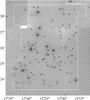 |
Fig. 1 Area of the Coma Berenices open cluster mapped by our TLS imaging survey. The total size of the surveyed area is ~22.5 deg2. Star symbols are probable Coma open cluster members, which are listed in Table B.1. |
We performed a basic reduction of the raw images including overscan correction, bias substraction, and dome flat-fielding following standard recipes in IRAF2. All the I-band images contained a prominent interference fringe pattern caused by night sky emission. These fringe strips were removed with a fringe mask constructed from the whole set of the I-band images. The R- and I-band images were then aligned where necessary and all were astrometrically calibrated using Graphical Astronomy and Image Analysis Tool software (GAIA) and the Hubble Guide Star Catalog (GSC v.1.2) as a reference. The GSC contains positions for most of the field stars down to magnitude V = 16. Each of our Coma CCD frames contained more than 30 reference stars evenly distributed across the field and the accuracy of the astrometric solution for individual images was better than  in both filters for both coordinates.
Cosmic ray hits (cosmics) were removed by combining each pair of RI-frames of the same sky field into one image and rejecting cosmics. The images also had several different kinds of artefacts and extended objects, which had to be discriminated from star-like objects. First of all, the sky location of the Melotte 111 cluster overlaps with the well-known extended galaxy cluster located in Coma Berenices and many resolved galaxies are visible in the obtained frames. In addition, some of the frames were contaminated with tracks from satellites and extended images of slow-moving objects (such as asteroids). Another source of extended artefacts is the bright stars of the cluster: their saturated images caused spikes that blocked some areas around these stars and did not allow us to detect faint objects lying in the vicinity of these spikes. In addition, the bright stars were accompanied by so-called Schmidt ghosts, which have to be separated from star-like objects. To detect all the star-like objects in the frames and separate them from the artefacts and extended objects, we used the following procedures.
First, the positions of all sources were extracted from the images (combined from RI-frames and cleared of cosmics) using the Source Extractor (SExtractor) software (Bertin & Arnouts 1996). An advantage of this method is that it allowed us to extract parameters of an object characterising its extention. We used the radius of the Kron aperture (Kp, the typical size of the aperture) and the elongation to discriminate between point-like sources and extended objects. Instrumental magnitudes of all extracted sources were then extracted based on the measurement of the point spread function (PSF) using the daophot package of IRAF. Finally, we converted the instrumental magnitudes into RI-band magnitudes using photometric standards observed in Landolt’s selected areas (“all-sky” method, see Sect. A.1).
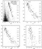 |
Fig. 2 I − (R − I) (top left), I − (I − J) (top right), I − (I − Ks) (bottom left), and J − (J − Ks) (bottom right) colour − magnitude diagrams of optically selected candidates (points) from the TLS and 2MASS/UKIDSS surveys. In all CMDs, we show 500 Myr NextGen isochrones shifted to the distance of the Coma open cluster as solid lines; the same age DUSTY isochrones (lower solid line) are shown in the I − (I − J) and I − (I − Ks) CMDs. The vertical line labelled with stellar mass (M⊙) is the mass scale according to the NextGen (Baraffe et al. 1998) models. The DUSTY isochrones in I − (I − J) and I − (I − Ks) are also marked with stellar mass. The two dashed lines display the uncertainty in the RI-photometry (PSF photometric errors only), which grows with magnitude. The upper horizontal line shows the stellar/substellar boundary and the lower line indicates the lithium burning limit. Field objects (points) from two CCD frames are shown. All objects around the I − (R − I) isochrone have been included in the list of candidates and thus the non-candidates are represented here for demonstration only. Five brown dwarf candidates are located close to or in the substellar domain. |
3. Selection of very low-mass stellar and brown dwarf candidates
For the photometric selection of the Coma open cluster VLM/BD member candidates, we compared their position on the I − (R − I) colour − magnitude diagram (CMD) with the NextGen model isochrones for solar metallicity provided by Baraffe et al. (1998). All of the 55 cluster fields contain between 4000 and 8000 objects, and in total about 290 000 objects were detected by SExtractor in the R,I-bands and plotted in the I − (R − I) diagram. The NextGen isochrones for ages of 400 or 600 Myr are not very different from each other and so we used a mean isochrone (500 Myr) to help us distinguish the Coma member candidates from foreground dwarfs (solid curve in Fig. 2). The isochrone was shifted to the Coma open cluster distance (m − M = 4.73). Interstellar reddening in the direction of the Coma open cluster is very low (Feltz 1972) and can be neglected. Figure 2 presents our I − (R − I) CMD, and the selected VLM/BD member candidates are marked as larger dots.
The two dashed curves on both sides of the isochrone display the 1σ photometric errors (PSF photometric errors only) increasing with magnitude. For the selection of the candidates, we started with all objects within a 1.5σ wide strip. The rapidly increasing amount of objects blueward of our blue boundary shows that the pollution of our sample with field objects may be an issue. There are also a number of objects located redward of our red boundary, especially in the upper part between I = 14.5 and 18, and we included them in our initial sample.
These red objects could be background dwarfs, distant galaxies, or red giants, although giants are highly improbable at such a high Galactic latitude. This observed displacement towards the red could be caused by the depth of the cluster (~0.15 mag) and binarity of the objects. Binary members can lie up to 0.75 mag above the single star sequence (Casewell et al. 2006). Unfortunately, we cannot identify the source of this reddening using only of the CMDs. Therefore, all these reddish objects were initially included in our list as potential cluster members. In this way, more than one hundred member candidates in the magnitude interval 14.5 < I < 20 were listed in the studied area of the Coma Berenices open cluster. These were then subjected to further checks, which are detailed in the following.
Non-members of the Coma open cluster with high proper motions.
3.1. Two-Micron All-Sky Survey
We cross-referenced all our initial candidates against the Two-Micron All-Sky Survey (2MASS, Skrutskie et al. 2006) using a match radius of 2 5 and derived JHKs photometry for almost all our candidates, except for the six faintest objects. These six objects were then successfully cross-identified with objects in the UKIDSS survey using a search radius of 0.1 arcmin. We combined the derived NIR-photometry with our I-magnitudes into the three additional CMDs (see Fig. 2) of I − (I − J), I − (I − Ks), and J − (J − Ks). These diagrams together with theoretical NIR-isochrones from Baraffe et al. (1998) enable us to constraint the contaminants. We consider an object as a contaminant if its colour indices are bluer than predicted by the NIR-isochrones by 0.2−0.25 mag in at least two of these three NIR CMDs. After this inspection, we excluded 35 objects that were clear outliers in these diagrams and are therefore probably non-members of the cluster.
As for the I − (R − I) diagram, the 500-Myr IR-isochrones from Baraffe et al. (1998) are shown in Fig. 2 as solid curved lines, two dashed lines at both sites of the isochrones indicate the photometric uncertainty with a 1σ-error. One can see that the scatter in the colour indices of these NIR CMDs is larger than the corresponding photometric uncertainty, but nevertheless these rectified diagrams do not contain prominent outliers. Nonetheless, some objects are shifted towards blue indices within a single NIR CMD. For instance, object H3-258 located in the top part of the I − (I − J) CMD is too blue for a main I − (I − J)-sequence of the Coma open cluster, but other NIR-diagrams show that its colour indices are red enough to place this object close to the corresponding cluster colour sequences. Thus, we cannot completely exclude this object as a cluster candidate.
In the CMDs in Fig. 2, one can also see that many of the VLM candidates lie on the blue side of the colour − magnitude isochrones. Various theoretical calculations show that very cold low-mass objects can be bluer than the NextGen model predicts because of the formation of dust in the atmospheres of these objects (Baraffe et al. 2003). The lower solid line in the I − (I − J), I − (I − Ks) CMDs (Fig. 2) displays a 500 Myr isochrone from DUSTY models of Baraffe et al. (2003), which take the possibility of dust formation into account. Therefore, these DUSTY models may be more appropriate for the lowest mass stars and BDs with Teff > 1300−1400. Moreover, in these cold atmospheres a dust equilibrium can be unstable and the dust may fall to lower atmospheric layers, which can result in a sudden change in the infrared indices toward bluer colours (Bouvier et al. 2008). Taking photometric uncertainty into account, the location of the substellar cluster members in NIR CMDs may thus span a large range of colours, placing the members from the NextGen isochrone bluewards.
3.2. Proper motion as a selection criterion
As the next step in rectifying our sample from back- and foreground objects, we used information about the proper motions of the objects. Unfortunately, the mean proper motion of the Coma open cluster is about 10 mas yr-1 (van Leeuwen 1999), which is very close to that of Galaxy field stars. Therefore, Coma members cannot be discriminated from the field stars based on their proper motions. However, we can exclude objects with high proper motions and therefore inconsistent with membership of the Coma Berenices open cluster from our list.
Lépine & Shara (2005) published a catalogue of high proper motion stars (LSPM-catalogue) in the northern hemisphere with annual proper motions larger than 015 yr-1, that also covers stars in the Coma open cluster region. Examining the LSPM-catalogue, we identified nine high proper motion objects among our candidates and therefore these objects are probably not Coma open cluster members. We list these objects in Table 1 and excluded them from our list of candidates. In this table, the coordinates of these objects obtained from our survey and proper motions taken from the LSPM-NORTH catalogue are presented. We also performed a search for high proper motion objects in the USNO-B1.0 catalogue with annual proper motions larger than 015 y-1 as a selection criterion and identified only one object (1184-0204433) that exceeds this limit (Table 1).
Photometric brown dwarf candidates.
3.3. Selection by object shape
We should take into account that some of the selected objects can be distant unresolved galaxies. Therefore, as a test for these background objects, we analysed a full width at half maximum (FWHM) distribution of the selected candidates to discriminate between point-like sources and star-like galaxies. In practice, we calculated the average FWHM of 20−30 unblended and unsaturated bright stars with well-shaped profiles for each frame and excluded any of our candidates whose FWHM deviated considerably from this average FWHM. As an upper limit to this deviation, we defined a region of width 3 × σ where σ is the FWHM of the normal distribution of the FWHMs of our sample, with  in our case. We rejected only candidates that did not comply with this criterion in both the R and I passbands. As a result, 12 objects were excluded from our list.
4. Spectroscopy
We obtained low-resolution optical spectroscopy of 14 low-mass member candidates from our photometric sample. Spectra of 12 objects were obtained with the faint-object Nasmyth spectrograph on the 2-m TLS telescope during February and May 2007. This spectrograph used the same SITe 2048 × 2048 CCD chip as used for the imaging, and a V200 grism was chosen, which produced a spectrum covering the spectral range from 3600 Å to 8700 Å with a dispersion of 3.3 Å pix-1. The spectra could only be used up to 7700 Å, where the second order spectrum starts to overlap with the first order. The exposure time was 600 s, but several objects were observed twice for a total of 1200 s. The exposure times yielded a signal-to-noise ratio (S/N) of about 15 per resolution element at 6800 Å, which was enough to classify the spectra with an accuracy of ± 1 spectral subclass. Two of the faintest spectra had S/N of ≈ 10 per resolution element, leading to classification errors of 1.5 subclasses.
Spectroscopic observations of two more VLM candidates were obtained on April 28, 2007 with the MOSCA spectrograph at the 3.5-m telescope of the German-Spanish Observatory on Calar Alto (CAHA, Spain). The R500 grating provided a spectrum covering the wavelength range from 5400 Å to 10 000 Å with a dispersion of 2.8 Å pix-1. As for the TLS spectra, the red part of the CAHA spectra was contaminated with the second order spectrum. Since the CAHA targets were fainter than the TLS targets, an exposure time of 600 s yielded a similar S/N for both telescopes. For both series, the spectrophotometric standard stars Feige 66 and Feige 67 (Massey et al. 1988; Massey & Gronwall 1990) were observed.
The TLS and CAHA spectroscopic frames were bias-subtracted and flat-fielded using standard procedures in IRAF. Domeflats and dark exposures were obtained to achive this goal. We also removed the few cosmics in the frames using the Laplacian algorithm of cosmic ray identification developed by van Dokkum (2001). Wavelength calibration of the TLS spectra was done using bright sky lines on the spectra, while the CAHA spectra were wavelength-calibrated with independently taken Ar+Mg+Ne arc-spectra. The sky lines were then removed from the spectra by background subtraction and the individual one-dimensional (1D) spectra were extracted. Finally, an absolute flux calibration of both series of 1D-spectra was done with the spectrophotometric standards.
5. Results and discussion
We surveyed 22.5 deg2 of the central area of the Coma open cluster, which is a little bit larger than the area of the Coma open cluster tidal radius of  derived by Casewell et al. (2006). The selection procedures described in the previous sections resulted in 82 cluster candidate members, which are listed in Table B.1. This table contains our RI-photometry of all the objects as well as their 2MASS (UKIDSS) JHKs photometry. Their local names are given according to the field name (the first two letters) and object number in that field. Cross-identifications with 2MASS sources are also given. Coordinates of the objects extracted from the TLS frames are based on the J2000 epoch of the Guide Star Catalog 1.0.
We estimated the completeness of our survey in the R and I-bands as described in Caballero et al. (2007). They stated the completeness as the magnitude where the number of detected sources per magnitude interval stops increasing with a fixed power law of the magnitude, N(m) ∝ mp. Our calculation shows that our survey is complete to 21.5 in the R-band and 20.5 in the I-band. The limiting magnitude of our RI-survey is about 1.5−2 mag fainter than the completeness magnitude, i.e. the limiting magnitude is 23 mag for the R-band and 22.5 for I. The estimates of these photometric characteristics of our survey are based on the analysis of all detected star-like sources. As one can see from these values, the I-band magnitudes of our faintest candidates are within the I-band completeness of our survey, although the faintest candidates (R − I ~ 2.5−3) have R-magnitudes below the completeness limit. This means that some faint objects with colour indices consistent with brown dwarfs detected in the I-images may not have an R-counterpart. To verify this, we cross-referenced all objects detected in the I-images with R-frames and we did not find any I-objects without an R-counterpart. Hence, our detection method worked well and we did not miss any of the reddest objects.
The I − (R − I) CMD of the final candidate sample is shown in Fig. 2 together with the 500 Myr NextGen model isochrone shifted to a distance modulus of m − M of 4.73 (88 pc). The cluster candidates span from I ~ 14.5 to 20, covering the mass range from 0.21 M⊙ to 0.06 M⊙ (65 Jupiter masses), which corresponds to spectral types from M2 down to L0 (theoretical stellar isochrones labelled by mass in the I − (R − I) panel in Fig. 2). The stellar-substellar boundary for the Coma open cluster assuming its age of 500 Myr lies at I ~ 19.1 in the CMD (dashed horizontal line). Most of our candidates (77) seem to be low-mass stars (0.08−0.20 M⊙). Four objects are located around the substellar borderline; one lies in the substellar domain (M ≤ 0.075 M⊙) and is located close to the limit of lithium burning, which occurs at I ~ 20 for the cluster. Since the photometric error is large at these magnitudes we are unable to ascertain whether these objects lie under this boundary. Therefore, these five candidates to be brown dwarfs can occupy the area restricted in the I − (R − I) diagram by the deuterium burning limit (horizontal solid line) and the lithium burning limit (dotted line) adopted for the Coma open cluster age (500 Myr); these objects are listed in Table 2. The resulting I − (R − I) CMD showed that the number of objects located around the isochrone is not as large as in the CMD based on 2MASS photometry (see Fig. 2 in Casewell et al. 2006), which was definitely contaminated by field objects, especially in its bottom part.
All the 82 candidates can be qualified as possible members of the Coma open cluster according to their near-infrared CMDs combined from I and 2MASS photometry, namely I − (I − J), I − (I − Ks), and J − (J − Ks). As noted above, these candidates cannot be discriminated from field stars of the Galaxy owing to the similarities between their proper motions.
5.1. Field object contamination
Analysing 2MASS photometry, Casewell et al. (2006) found that photometric VLM candidates of the Coma open cluster are contaminated with a sizable number of field objects, especially for objects with magnitudes Ks > 12. Ford et al. (2001) suggested that the contamination level among the low-mass stars can be as high as 40%. We should therefore also try to estimate the level of contamination in our sample.
Our remaining candidates may also be contaminated by back- and foreground objects, most of which are probably red main-sequence dwarfs from the thin disk of the Galaxy. An estimate of the number of contaminating field stars may be obtained from the Besançon galaxy model (Robin et al. 2003), which gives star counts depending on their brightness, colours, and Galactic coordinates. The simulation of an I − (R − I) CMD for a 1-deg2 field centred on Melotte 111 (l = 222.5,b = 83.4) gives about 28 objects within our error stripe around the cluster isochrone of 500 Myr. Scaling the number to the covered area (22.5 deg2), we get an estimate of about 600 stellar objects in our selected colour − magnitude space, while we found only 82 candidates in this region. This indicates that the stellar contamination may be quite high. To check the stellar density around the Coma Berenices open cluster, we repeated the simulations for the same size fields (1 deg2) with longitude ± 10deg in both directions from the centre of the Coma open cluster and at the same latitude. We found similar results for star counts around the isochrone of 500 Myr: 30 stars for the field with (l = 212,b = 83.4) and 24 for (l = 232,b = 83.4). This means that there is no prominent deviation from the mean field star density in this area and this wide cluster is probably not included in the Besançon galaxy model.
A problem with the contamination simulation can be the faintness of the selected objects. Robin et al. (2003) note that the Besançon model closely reproduces the observed star counts at V-magnitudes between 12 and 24. At fainter magnitudes, deviations are found and the model predictions strongly depend on the assumed initial mass function (IMF) at low masses, which is still very uncertain. In our simulation, 15 of the 28 contaminating objects lie at I = 19 and fainter. They have (I − R)-colour excesses of about 2.5, and for V − R = 3, which is typical of these red objects, the contaminants will be fainter than V = 24.5.
This situation shows very clearly why it is so difficult to find VLM members of the Coma open cluster in comparison with more compact open clusters. The Coma open cluster is large on the sky and the surface density of VLM members is low there. For either the Pleiades or σ Ori clusters, this is different: the surface density of the members is much higher owing to the smaller angular extent of the clusters, thus the detection of their members is easier.
5.2. Spectroscopic classification
Fourteen candidates were spectroscopically observed with low resolution (12 objects at TLS and 2 objects at CAHA). The spectra of three objects covering wavelengths from 5500 Å to 7650 Å are shown in Fig. 3. The spectra of most of the objects (12 of 14) exhibit prominent wide TiO and CaH molecular bands, which prove that these objects are stars and not distant unresolved galaxies. Two objects (F9-2311 and F6-318) have quite noisy spectra and their TiO molecular bands are not so prominent. However, these bands are still visible (deep depressions at 6800 Å and 7150 Å between wide peaks at 6650 Å and 7040 Å), which also indicates the stellar nature of these objects. We also noted the presence of the following atomic features – resonance doublets K I λ 7665, 7699 Å and Na I λ 8183, 8195 Å, which are blended at our low spectral resolution and contaminated with telluric bands. We found Li I λ 6708 Å in neither absorption nor emission in any spectrum. Four of the 14 objects display an Hα line in emission, which might be evidence of their youth and increases the probability of their cluster membership.
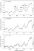 |
Fig. 3 TLS optical spectra of three VLM stars. The spectra are normalised to the flux at ~7500 Å. The vertical labelled lines in the C6-1135 spectrum show the positions of the narrow-band spectral indices from Gizis (1997, see Table 3). |
Narrowband indices in the classification scheme of Gizis (1997).
We do not expect to find distant background M-type giants in the direction of the Coma open cluster owing to the high latitude of the cluster. Nevertheless, we need to implement a test to distinguish dwarfs from giants to be sure that all our candidates are genuine dwarfs. Jones (1973) suggested a simple method measuring fluxes with narrowband filters (FWHM = 30 Å) centred on 6076, 6830 Å (CaH), 7100 Å (TiO), and 7460 Å. A plot of the CaH/TiO ratio, m(6830) − m(7100), against the colour m(6076) − m(7460) shows that there is a clear separation between dwarfs and giants in these indices: dwarfs have only positive CaH/TiO ratios (m(6830) − m(7100) > 0), whereas all giants have negative ones. Computing the same parameters from our spectra, we found that the CaH/TiO ratios for all the candidates is clearly positive confirming their dwarf nature.
Spectral classification of 14 TLS candidates.
To determine the spectral types of the BD/VLM candidates, we used two different methods. The first method is based on the analysis of the low-resolution spectra using the dwarf classification scheme of Gizis (1997). This method examines the strength of several strong molecular absorption bands of titanium oxide TiO and calcium hydride CaH sensitive to temperature and hence, to spectral type. Wavelength regions for the bands and continuum points chosen by Gizis (1997) and used in our current work are presented in Table 3. The bandstrength indices were calculated from Rind = FW/FS1 for the TiO 2 and CaH 2, 3 indices, and Rind = FW/(FS1 + FS2)/2 for the CaH 1 index, where FW is the flux in the region including the feature and FS is the flux in the pseudo-continuum region. One advantage of this method is that the bandstrengths are determined by measuring the ratio of fluxes within a small wavelength region centred on the feature of a nearby pseudo-continuum point. Therefore, only an accurate relative flux calibration is required, rather than an absolute calibration (and hence photometric conditions). To be sure of the accuracy of the spectroscopic reduction, we calibrated all spectra in term of absolute fluxes and applied this method to the flux-calibrated spectra.
Calculated spectral indices TiO 5 and CaH 1 − 3 for our 14 candidates are listed in Table 4. The indices were converted into the spectral types of the stars according to Eqs. (1)−(3) from Gizis (1997). These are effective in assigning spectral types to dwarfs over a range K7−M6 (with the exception of the CaH 1 index, which saturates at ~M3). All our spectroscopically observed candidates (located in the upper part of the CMD diagrams, see Fig. 2) are expected to have spectral types of early-M, hence this method is suitable for the spectral classification of our sample.
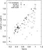 |
Fig. 4 The spectral indices TiO 5 − [CaH 2 + CaH 3] of the TLS candidates (star symbols). Three sequences from Gizis (1997) are shown: main-sequence disk dwarfs dKV − dMV (filled circles), subdwarfs sdK − sdM (open circles), and extra-subdwarfs esdK − esdM (open squares). |
The second method that we used employs the luminosity–spectral type calibration constructed by Kraus & Hillenbrand (2007), which is based on a large sample of stellar SEDs. This calibration sequence allows us to estimate the spectral type (SpT) of a star based only on its optical/NIR photometry. The results of this classification are presented in Table B.1. The second last column displays the spectral type derived from the TLS I-band magnitudes and the last column is an average result of three estimates from 2MASS JHKs (for objects lacking 2MASS photometry, JHK photometry from UKIDSS was used.). Spectral-type sequences derived from JHKs are quite self-consistent and SpT estimates of a star based on these bands agree very well: the SpT values are equal to or lie within one spectral subclass. At the same time, JHKs-SpTs are systematically later than the ones calculated from the I-band. Moreover, this difference increases towards later SpT objects. This may imply that our I-band calibration has some bias with respect to the 2MASS JHKs-system.
To compare the photometric spectral calibration with the spectral types based on the spectra, we put the JHKs-photometric SpT of objects observed spectroscopically in the last column of Table 4. First of all, for objects classified with both approaches SpT values derived from spectral indices in general have later SpT than those based on photometry. Considering this result in more detail, one can say that the SpT determined from both methods agree well (to within half of a Sp-subclass) for 4 of the 14 objects, whereas for 7 objects the SpT values agree to within 1.5 subclass. For only three objects (B6-1509, C7-751, and G5-1311) do the spectral indices represent SpT values later by 2 subclasses (and larger) than those derived from photometry. The S/N of the spectra of two of these stars (B6-1509 and C7-751) is large enough for us to derive reliable indices, but the spectrum of G5-1311 is quite faint and the error in its determination may be higher. In general, the photometric SpT values cover a smaller range (from M4 to M6) than the SpT calculated from the indices (M4 − M8).
The spectral indices also allow us to distinguish MV dwarfs (dM) from dwarfs with low metallicity namely subdwarfs (sdM VI) and extra-subdwarfs (esdM) that belong to the old population of the thin Galaxy disk. According to the Gizis (1997) scheme, the separation between the stellar subclasses can be done by analysing their distribution in three diagrams: TiO 5 vs. CaH 1, TiO 5 vs. CaH 2, and TiO 5 vs. CaH 3. However, a simplified version of this classification based on a single diagram of TiO 5 − [CaH 2+CaH 3] was later commonly used for this analysis (Lépine et al. 2003, 2007). According to these papers, this classification scheme is essentially equivalent to the original Gizis (1997) system. Following this, the diagram of TiO 5 vs. CaH 2+CaH 3 indices is shown in Fig. 4. Our 14 objects are plotted with asterisks. Three sequences of dwarfs are also overplotted according to spectral indices taken from Gizis (1997): main-sequence K-M dwarfs (filled circles), sub-dwarfs (empty circles), and extra-subdwarfs (empty squares) of the same spectral class range. However, we should take this test with caution because the separation between the dwarf V and VI sequences in the TiO−CaH index diagram is not significant. Nevertheless, the positions of the three stellar sequences in this diagram allows us to discriminate MV-dwarfs from both subdwarfs and extra-subdwarfs, even for objects with SpT > M3. In addition, one can see that a number of our candidates are located above the dK-dM sequence. At the same time, MV-dwarfs from Gizis’ list also have a bump on the TiO 5 − [CaH 2+CaH 3] diagram and their distribution overlaps with our objects.
In the TiO 5 − [CaH 2+CaH 3] index diagram, only two objects (B6-1509 and G5-1311) lie in the area of the sdM-dwarfs. We cannot exclude, however, that these objects belong to the MV-dwarfs because both objects are located close to the MV-star sequence in this diagram, hence the possibility that these objects are dwarfs with solar metallicity cannot be ruled out.
Finally, we can conclude that most of our spectroscopically observed candidates can be classified as MV-dwarfs, hence their spectroscopic parameters are consistent with Coma open cluster membership.
5.3. Comparison with previous studies
Previous studies have shown that Melotte 111 has a relatively small amount of members compared to the Hyades, which is another open cluster with a similar age. In total, the number of known cluster members with M ≳ 1 M⊙ seems to be about 50 objects (Argue & Kenworthy 1969; Deluca & Weis 1981; Bounatiro & Arimoto 1993). Casewell et al. (2006) performed an analysis of objects in about 50 deg2 of the Coma open cluster area using 2MASS photometry and proper motions from USNO-B1.0. They confirmed 45 previously known members of the Coma open cluster in their survey. Casewell et al. (2006) also identified 60 new cluster candidate members with masses in the range 1.01 > M ⋆ > 0.27 M⊙. Another survey for new cluster members was done by Kraus & Hillenbrand (2007), who also used archival surveys (SDSS, 2MASS, USNO B1.0, and UCAC-2.0). They compiled proper motion and photometry in the Coma open cluster region from these databases and published a list of 149 member candidates with membership probabilities of ≥ 50% down to M ⋆ ~ 0.12 M⊙. Of these candidates, 98 have membership probabilities of > 80%. As mentioned above, the brightest objects from our survey correspond to stars with masses ~0.2 M⊙. Thus, our sample overlaps with the list of Kraus & Hillenbrand (2007). Taking photometric errors and consequential errors in the mass determination into account, our survey may overlap with Casewell et al. (2006) over only a marginal mass range around 0.25 M⊙.
A comparison of our sample with that of Kraus & Hillenbrand (2007) shows that there is good agreement among the selected candidates. The Casewell et al. (2006) survey covers a larger area than our study and we selected all stars with spectral types later than SpT = M3 from their list in the area covered by our survey. We identified 22 stars in this region of which 9 stars with SpT between M3 − M7 are recovered in the TLS survey (marked in Table B.1). Seven objects listed by Kraus & Hillenbrand (2007) are not detected in our study because they are too bright. We initially selected another 5 stars as member candidates, but then excluded them from our list because their image profiles exceed a saturation threshold of 55 000 ADU (see Sect. 2). The last star of the 22 objects (J12310816+2416351, SpT = M7.3) was not detected in the TLS surveys probably because it has a fainter star in its close vicinity. This object was presumably not resolved by SExtractor and was excluded from our list as an extended object. Finally, we compared our candidate list with the Casewell et al. (2006) survey, but no common objects were found. We suggest that this is because the bottom mass limit of the Casewell et al. (2006) survey really does not overlap with our survey.
Comparing our object sample with known Coma members of higher mass (Kraus & Hillenbrand 2007) in CMDs based on 2MASS and TLS photometry, we see that all the objects lie well in accordance with these CMDs and form a cluster stellar sequence from the brightest cluster members to the faintest member candidates. Therefore, combining our photometrically selected objects with the previously found members, we are now able to extend the mass function down to ~0.06 M⊙.
5.4. Mass function
Odenkirchen et al. (1998) estimated that the Coma open cluster has the total mass in the range of 30 M⊙ to 90 M⊙ in a core with a tidal radius of ≈5−6 pc. Kraus & Hillenbrand (2007) calculated that the total stellar population of the Coma open cluster consists of 145 ± 15 stars earlier than M6 corresponding to a total mass of 112 ± 16 M⊙. These estimates are much less than that estimated for the Hyades, 300 − 460 M⊙ (Oort 1979; Reid 1992), which is a cluster of similar age. Kraus & Hillenbrand (2007) found that the mass function of the Coma open cluster can be fit, over the mass range 0.1 − 1 M⊙, with a single power-law dN/dm ∝ m − α with α = 0.6 ± 0.3.
Odenkirchen et al. (1998) found that the Melotte 111 luminosity function in the cluster centre sharply falls beyond MV = 4.5 (V = 9.2) towards fainter magnitudes, indicating that the cluster core has probably lost its lower mass members. This means that the mass function must also decline. However, Ford et al. (2001) analysing the population of the Coma open cluster core concluded that the luminosity function may be flatter than derived by Odenkirchen et al. (1998). On the other hand, Casewell et al. (2006) analysing the mass function down to 0.27 M⊙ concluded that the mass function is still well-traced at this mass and hence lower-mass members can be found. Kraus & Hillenbrand (2007) also found that the mass function law is quite shallow for spectral types up to M6 and a total depletion of cluster members must occur below ≈0.12 M⊙.
We estimated the masses of all the objects listed in Table B.1 assuming that the objects satisfying all of our selection criteria are very low-mass members of the Coma open cluster. Masses of the candidates were calculated by linear interpolation of the relationship between luminosity and the theoretical masses of Baraffe et al. (1998). To improve the accuracy of our determination, we estimated the masses for both the I- and Ks-band. Comparing mass values obtained from the two bands, we found that these values are not completely self-consistent and the difference increases slowly from lower to higher masses. Hence, we fitted this trend linearly and derived the final mass values according to this relation.
As a result, we found that these objects cover a mass range from 0.2 M⊙ to 0.06 M⊙, i.e from low-mass stars to substellar objects, assuming that they are cluster member. The derived masses were binned with a step of 0.02 M⊙ and the resulting mass spectrum is presented in Fig. 5. An error bar of mass bins comes from the uncertainties in the photometric measurements. The straight line overplotted on this diagram represents a mass function of dN/dm ∝ m − α where α = 0.6 over the mass range of 0.05−0.25 M⊙, which is similar to that derived for the Pleiades (Moraux et al. 2003). More recent estimations of α for the Pleiades can be obtained from Stauffer et al. (2007) and Lodieu et al. (2012). According to Stauffer et al. (2007), the α is about 0.8 for masses below 0.1 M⊙, whereas the study of Lodieu et al. (2012) shows that the mass function is quite flat over the mass range 0.03−0.20 M⊙, i.e. α ~ 0. Therefore we adopted α = 0.6 from (Moraux et al. 2003) as a compromise value. The Pleiades have an age of ≈120 Myr and the dynamical evolution of this open cluster still appears to have had little effect on its present-day mass distribution (Moraux et al. 2003). The same value of α was derived in Kraus & Hillenbrand (2007) for the Coma open cluster, but in the range 0.9 > M ⋆ > 0.12 M⊙.
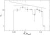 |
Fig. 5 The present-day mass function, Ψ(m) = dN/dm, for the Coma Berenices cluster from 0.2 M⊙ to 0.06 M⊙. Each mass bin with an error bar has a width of 0.02 M⊙; the error bars are based on the photometric uncertainties. The horizontal line is the mass function for the mass range 0.06 − 0.14 M⊙ derived from our data. For comparison, the Pleiades mass function dN/dm ∝ m-0.6 (inclined solid line) fitted over the mass range 0.05 − 0.25 M⊙ (Moraux et al. 2003) is overplotted. The limiting magnitude of the TLS survey (I = 22.5) corresponds to objects with mass ~0.05 M⊙. |
In the mass distribution in Fig. 5, one can see that there is an apparent deficit of objects in the first mass bin (at 0.21 M⊙). This is probably due to some members in this bin being missed because of saturation effects on our CCD frames. At the same time, the low-mass edge of this histogram in the substellar domain lies within the I-band completeness (205) of our survey. If we exclude the first bin, the mass function in the region with lower masses shows a flatter distribution. Going into detail, we can divide this mass spectrum into two parts: the first section is from 0.2 M⊙ down to 0.14 M⊙ and the second one is from 0.14 M⊙ down to 0.06 M⊙. In the first section, the mass spectrum rises gradually and can be fit with a mass function of slope α = 0.6, which coincides with the result of Kraus & Hillenbrand (2007). For objects with masses between 0.14 M⊙ and 0.06 M⊙, this mass function then becomes almost horizontal with α ≃ 0.
Such a shallow mass function is significantly shallower than a Salpeter IMF (α = 2.35), which was found for the mass range 1−10 M⊙. The Coma mass spectrum is also shallower than a present-day mass function for nearby field M-dwarfs (α ~ 1.3 for 0.1 < M < 0.7 M⊙Reid et al. 2002). However, the slope of the mass function of the stellar population in open clusters and stellar associations decreases when we consider stellar masses below 2−3 M⊙ (Hillenbrand 2004). In this context, it is interesting to compare the mass function law of the Coma open cluster with similarly aged open clusters: the Hyades and Praesepe. The mass function of the open cluster Praesepe (age of ~ 500 Myr) in the range of 0.1−1 M⊙ was fitted by a single power law with α = 1.4 (Kraus & Hillenbrand 2007) (or α = 1.1 from Baker et al. 2010), which is higher than for the Coma open cluster in the same mass range. For the Hyades, Bouvier et al. (2008) found a much lower value of the index over 0.05−0.2 M⊙ namely α = −1.3, which can be explained as a result of the dynamical evolution of the cluster. On the other hand, young open clusters also show different mass function laws. For example, the mass spectrum of the young (~5 Myr) cluster σ Orionis becomes flatter at about 0.2 M⊙ (see Fig. 8 in González-García et al. 2006) and extending to substellar objects it rises only with an exponent α = 0.6 − 0.8 (Béjar et al. 2001; González-García et al. 2006). Another young cluster located in the λ Orionis star-forming region (Collinder 69), was found to have a mass spectrum slope of ~0.3 for 0.01−0.7 M⊙ (Bayo et al. 2011).
On the other hand, our sample may still be contaminated with a number of background objects, and after weeding out these objects the difference between the initial and present-day mass functions could become larger. In addition, since a number of objects could be unresolved binaries, their masses will represent the sum of both components and this will also distort the mass distribution. Thus, we suspect that the Coma open cluster mass function at its low-mass end is more depleted compared to the higher mass section of the mass function. Since our survey mapped quite a large area (22.5 deg2), it my well have also caught low-mass objects that had already “evaporated” from the tidal core of the Coma open cluster, but at this time we cannot distinguish these objects from those still bound to their host cluster.
6. Summary
We have performed a wide R,I-imaging survey of 22.5 deg2 around the core of the Coma Berenices open cluster (~500 Myr; r = 88 pc). The estimated limiting magnitudes of this survey are 23 for R-band and 22.5 for I. We initially selected potential cluster members based on this RI photometry. We then used 2MASS JHKs photometry to weed out contaminating objects. We continued with proper motion information to identify contaminating objects with inconsistent proper motions and used the shape to identify small galaxies. This led us to a final list of 82 cluster member candidates. According to the theoretical models of Baraffe et al. (1998), these objects range from 0.2 M⊙ to 0.06 M⊙ for the distance and age of the cluster. Five objects are estimated to have masses close to or below the substellar boundary of ~M ⋆ = 0.075 M⊙ and hence might be brown dwarfs.
Follow-up spectroscopy of 14 candidates was obtained at the 2-m TLS and 3.5-m CAHA telescopes. These low-resolution spectra in the far-red with a dispersion of ~3 Å pix-1 allowed us to perform a spectral calibration and a determination of their luminosity class. The spectroscopic features of all observed objects show that they are dwarfs and 12 are probably main-sequence stars (MV-dwarfs) with solar metallicity. Four objects (~30% of the sample observed spectroscopically) display an Hα emission line that may be evidence of their relative youth (500 Myr). Our spectroscopy gives a spectral type and luminosity that are consistent with Coma open cluster membership for all 14 candidates. This suggests that the membership probability of the remaining objects may be high.
We conclude that we have excluded most of the foreground dwarfs from our survey using optical/NIR CMDs. With the obtained spectroscopy, we classified the spectra of 14 candidates and found no evidence of contamination by the background giants that are scarce in this direction. We cannot completely exclude, however, that our photometric sample may be contaminated by Galaxy field red dwarfs that could intermix with the genuine Coma open cluster members during 500 Myr evolution. We also cannot exclude that there are a number of field objects with anomalous colours that may be identified as potential cluster members.
We derived a mass spectrum (dN/dm ∝ m − α) in the mass interval of 0.21−0.06 M⊙ assuming that all our candidates are Coma open cluster members. Between 0.21 M⊙ and 0.14 M⊙, this mass spectrum can be fit with a mass function with a slope α = 0.6. For objects with masses of 0.14 − 0.06 M⊙, the mass function becomes flatter and horizontal. This may be a consequence of the gradual tidal “evaporation” of the lowest-mass members from the cluster during its dynamical evolution. Taking into account the low proper motion of the Coma open cluster members and the size of the mapped area, we concede that our survey may also have caught objects that had already left the tidal core of the cluster and are now in fact foreground/background objects.
Online material
Appendix A: Photometric system in the RI-passbands of the 2-m TLS telescope
The CCD camera at the Schmidt focus of the 2-m telescope of the TLS contains five filters of the Johnson-Cousins photometric system – UBVRI. Since we used only R- and I-bands, we discuss only these passbands here.
The TLS R-band of the camera is defined by a combination of three filter glasses (OG570/2 mm + KG3/2 mm + WG295/4 mm), whereas the I-band is reproduced with two filter glasses (RG780/3 mm and WG295/4 mm). The TLS RI-filter transmissions together with the SITe CCD sensitivity curve and Cousins/Bessel RI-passbands are shown in Fig. A.1. As one can see, the TLS R-filter reproduces well the original Cousins/Bessel R-passband designed for CCD-photometry (Bessell 1979), but the short wavelength cut-on of the TLS I-filter shifts it from the standard Cousins/Bessel I filter to 750 nm. The red edge of the I-bassband is open up to 1100 nm with over 90% transmission at wavelengths longer than 875 nm. Thus, a red fall-off is imposed by the 2k × 2k SITe detector passband.
A.1. Reduction of photometry
To transform the TLS instrumental magnitudes to the Johnson-Cousins standard system, we observed three Landolt fields – SA 101, 104, and 107 (Landolt 1992) – during all of the nights. Each of these fields contains several tens of standard stars. Our field of view included 28 standard stars in both SA 101 and SA 104 and 22 stars in SA 107. The SA-fields were observed at high and low zenith distances to correct our instrumental magnitudes for atmospheric extinction. Observations of an SA-field were on average repeated every 1.5 h. Because of the higher brightness of Landolt standard stars compared to our targets in Coma, the integration time of the SA fields was only 10 s (600 s for the cluster fields) and in the following reduction, fluxes of the standard stars were scaled to the exposure time of the cluster frames.
The calibration of the extracted instrumental magnitudes to the Landolt system was done in IRAF (“all-sky” method). We solved the transformation equations for standard stars of the form ![Mathematical equation: \appendix \setcounter{section}{1} \begin{eqnarray*} r_\mathrm{CA} &= R + ZP_R + A_R*XR + C_R*(R-I)\\[2mm] i_\mathrm{CA} &= R-(R-I) + ZP_I + A_I*XI + C_I*(R-I), \end{eqnarray*}](/articles/aa/full_html/2012/08/aa19314-12/aa19314-12-eq233.png) where R and R − I are the catalogue magnitude and colour of a standard star, ZPR and ZPI are zero-points of the R- and I-bands, AR and AI are the coefficients of atmospheric extinction in the proper bands, XR and XI are airmasses at a moment of observation, and CR and CI are the colour transformation coefficients. Solving the equations, we find the ZP and C coefficients and apply this solution to our programme stars, converting the TLS instrumental magnitudes to the Landolt system. Since we observed the standard stars every 1.5 h, we were able to check the atmospheric stability during the night. Our inspection showed that in some nights the extinction parameters changed considerably and we were not able to fit all observations of standard stars with the same equation. In these cases, we divided the observations into parts and fitted them separately.
where R and R − I are the catalogue magnitude and colour of a standard star, ZPR and ZPI are zero-points of the R- and I-bands, AR and AI are the coefficients of atmospheric extinction in the proper bands, XR and XI are airmasses at a moment of observation, and CR and CI are the colour transformation coefficients. Solving the equations, we find the ZP and C coefficients and apply this solution to our programme stars, converting the TLS instrumental magnitudes to the Landolt system. Since we observed the standard stars every 1.5 h, we were able to check the atmospheric stability during the night. Our inspection showed that in some nights the extinction parameters changed considerably and we were not able to fit all observations of standard stars with the same equation. In these cases, we divided the observations into parts and fitted them separately.
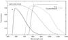 |
Fig. A.1 Filter responses and TLS SITe CCD sensitivity curve. The transmissions of the TLS photometric system are shown as thick solid lines for the R-filter, I-filter, and the SITe 2k × 2k CCD detector sensitivity curve. The dashed lines are RI-filter profiles from the Cousins/Bessel system (Bessell 1979). The red cut-off of the TLS I-passband is imposed by the red fall-off of the SITe CCD detector. |
At the same time, though we used Landolt standards to compute the photometric transformation, the resulting I-magnitudes are not in the Cousins system. As mentioned, this is due to the different passbands of the TLS and Cousins I-filter. Moreover, our set of Landolt fields contained stars mainly with R − I < 1.0, whereas our VLM/BD candidates have much redder colours, thus the colour transformation can be insufficient for those targets. Scholz & Eislöffel (2004) found that the I-band of the 2-m TLS telescope has a prominent shift relative to that of the Cousins system, which can reach 0.3 mag for objects with R − I > 1.5.
To correct this effect, we used the following procedure. We observed two Coma fields (C5 and D5) with three increasing exposure times of 10 s, 60 s, and 180 s. In the 10-s frames, we then selected several unsaturated stars photometrically observed by Deluca & Weis (1981) and Castelaz et al. (1991) as primary comparison stars. Using differential photometry, we computed magnitudes of all stars in these frames relative to each of the comparison stars. We selected about 10 fainter objects, averaged their magnitudes, and used them as secondary standards for the 60-s frames. To decrease the errors due to colour differences between the comparison stars and targets, we selected the secondary standards that are redder only at R − I ≈ 0.3 than their primary standards. In this way, we propagated the photometric system to our faint stars in the 600-s frames and finally, we determined magnitudes in 600-s C5- and D5-frames by differential photometry. In Fig. A.2 of the Appendix, we plotted the results against magnitudes calculated with the photometric method we used in the current work (“all-sky” method). As one can see, the difference between the methods for both the fields shows a clear dependence on the absolute values of the colour index. The difference is close to zero for stars with R − I = −0.5 and the correction for the “all-sky” method reaches  near R − I = 2.5. We then corrected the “all-sky” magnitudes using the obtained relationship. After this correction, the I − (R − I) and I − (I − J) CMDs (Fig. 2) show that in the range of the colour indices between 15 and 25 the corrected magnitudes agree with the 500 Myr isochrone from Baraffe et al. (1998).
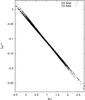 |
Fig. A.2 Comparison of I-band magnitudes computed with the differential photometry (Idiff) method and the “all-sky” method (used in the current work). The comparison is based on two Coma fields (C5 and D5). The difference between I-magnitudes calculated with these methods increases monotonically with growing R − I and reaches ~ 0.25 at R − I = 2.5. This difference could be due to different passbands of the TLS and Cousins/Bessel photometric systems and partly because the colours of the Landolt standards are not red enough for BD/VLM objects. |
Analysing the photometry, we also found a slight discrepancy between the photometric zero points of several CCD frames within the mosaic. The nature of the effects can be variable sky conditions, for instance, such as areas of thin cirrus that are almost invisible during the night time. A zero point correction was empirically computed from overlapping regions of frames using those obtained during good photometric conditions as references, and applied to the RI-magnitudes of the objects in our output photometric data.
Appendix B: Coma open cluster member candidates
In Table B.1, we provide a list of 82 optically selected Coma Berenices open cluster member candidates inferred from an I − (R − I) CMD that were selected for follow up based on 2MASS JHKs photometry and proper motion analysis.
RI- and 2MASS JHKs photometry of Coma open cluster member candidates.
A stellar mass function is an empirical function describing the mass distribution of a population of stars defined as Ψ(m) = dN/dm, where dN is the number of stars in the mass range (m,m + dm).
IRAF is distributed by National Optical Astronomy Observatories, which is operated by the Association of Universities for Research in Astronomy, Inc. under contract with the National Science Foundation.
Acknowledgments
J.E. and S.M. acknowledge support from the American Astronomical Society under the 2005 Henri Chretien International Research Grant. This publication has made use of data products from the Two-Micron All-Sky Survey, which is a joint project of the University of Massachusetts and the Infrared Processing and Analysis Center/California Institute of Technology and the United Kingdom Infrared Deep Sky Survey. This research has made use of the SIMBAD database, operated at CDS, Strasbourg, France, and of the IRAF software distributed by NOAO.
References
- Argue, A. N., & Kenworthy, C. M. 1969, MNRAS, 146, 479 [NASA ADS] [Google Scholar]
- Artyukhina, N. M. 1955, Trudy Gosudarstvennogo Astronomicheskogo Instituta, 26, 3 [NASA ADS] [Google Scholar]
- Baker, D. E. A., Jameson, R. F., Casewell, S. L., et al. 2010, MNRAS, 408, 2457 [NASA ADS] [CrossRef] [Google Scholar]
- Baraffe, I., Chabrier, G., Allard, F., & Hauschildt, P. H. 1998, A&A, 337, 403 [NASA ADS] [Google Scholar]
- Baraffe, I., Chabrier, G., Barman, T. S., Allard, F., & Hauschildt, P. H. 2003, A&A, 402, 701 [NASA ADS] [CrossRef] [EDP Sciences] [Google Scholar]
- Basri, G., & Martín, E. L. 1999, AJ, 118, 2460 [Google Scholar]
- Bayo, A., Barrado, D., Stauffer, J., et al. 2011, A&A, 536, A63 [NASA ADS] [CrossRef] [EDP Sciences] [Google Scholar]
- Béjar, V. J. S., Martín, E. L., Zapatero Osorio, M. R., et al. 2001, ApJ, 556, 830 [NASA ADS] [CrossRef] [Google Scholar]
- Bertin, E., & Arnouts, S. 1996, A&AS, 117, 393 [NASA ADS] [CrossRef] [EDP Sciences] [Google Scholar]
- Bessell, M. S. 1979, PASP, 91, 589 [NASA ADS] [CrossRef] [Google Scholar]
- Bounatiro, L., & Arimoto, N. 1993, A&A, 268, 829 [NASA ADS] [Google Scholar]
- Bouvier, J., Kendall, T., Meeus, G., et al. 2008, A&A, 481, 661 [NASA ADS] [CrossRef] [EDP Sciences] [Google Scholar]
- Caballero, J. A., Béjar, V. J. S., Rebolo, R., et al. 2007, A&A, 470, 903 [NASA ADS] [CrossRef] [EDP Sciences] [Google Scholar]
- Casewell, S. L., Jameson, R. F., & Dobbie, P. D. 2006, MNRAS, 365, 447 [NASA ADS] [CrossRef] [Google Scholar]
- Castelaz, M. W., Persinger, T., Stein, J. W., Prosser, J., & Powell, H. D. 1991, AJ, 102, 2103 [Google Scholar]
- Comerón, F. 2003, in Brown Dwarfs, ed. E. Martín, IAU Symp., 211, 53 [Google Scholar]
- de La Fuente Marcos, R., & de La Fuente Marcos, C. 2000, Ap&SS, 271, 127 [NASA ADS] [CrossRef] [Google Scholar]
- Deluca, E. E., & Weis, E. W. 1981, PASP, 93, 32 [NASA ADS] [CrossRef] [Google Scholar]
- Feltz, Jr., K. A. 1972, PASP, 84, 497 [NASA ADS] [CrossRef] [Google Scholar]
- Ford, A., Jeffries, R. D., James, D. J., & Barnes, J. R. 2001, A&A, 369, 871 [NASA ADS] [CrossRef] [EDP Sciences] [Google Scholar]
- García López, R. J., Randich, S., Zapatero Osorio, M. R., & Pallavicini, R. 2000, A&A, 363, 958 [NASA ADS] [Google Scholar]
- Gizis, J. E. 1997, AJ, 113, 806 [NASA ADS] [CrossRef] [Google Scholar]
- Gizis, J. E., Reid, I. N., & Monet, D. G. 1999, AJ, 118, 997 [NASA ADS] [CrossRef] [Google Scholar]
- González-García, B. M., Zapatero Osorio, M. R., Béjar, V. J. S., et al. 2006, A&A, 460, 799 [NASA ADS] [CrossRef] [EDP Sciences] [Google Scholar]
- Goto, M., Kobayashi, N., Terada, H., et al. 2002, ApJ, 567, L59 [NASA ADS] [CrossRef] [Google Scholar]
- Hillenbrand, L. A. 2004, in The Dense Interstellar Medium in Galaxies, eds. S. Pfalzner, C. Kramer, C. Staubmeier, & A. Heithausen, 601 [Google Scholar]
- Hodgkin, S. 2003, in Brown Dwarfs, ed. E. Martín, IAU Symp., 211, 183 [Google Scholar]
- Jameson, R. F., Dobbie, P. D., Hodgkin, S. T., & Pinfield, D. J. 2002, MNRAS, 335, 853 [NASA ADS] [CrossRef] [Google Scholar]
- Jones, D. H. P. 1973, MNRAS, 161, 19P [NASA ADS] [CrossRef] [Google Scholar]
- Kirkpatrick, J. D., Henry, T. J., & Irwin, M. J. 1997, AJ, 113, 1421 [NASA ADS] [CrossRef] [Google Scholar]
- Kirkpatrick, J. D., Dahn, C. C., Monet, D. G., et al. 2001, AJ, 121, 3235 [NASA ADS] [CrossRef] [Google Scholar]
- Kraus, A. L., & Hillenbrand, L. A. 2007, AJ, 134, 2340 [NASA ADS] [CrossRef] [Google Scholar]
- Landolt, A. U. 1992, AJ, 104, 340 [NASA ADS] [CrossRef] [Google Scholar]
- Lépine, S., & Shara, M. M. 2005, AJ, 129, 1483 [NASA ADS] [CrossRef] [Google Scholar]
- Lépine, S., Shara, M. M., & Rich, R. M. 2003, ApJ, 585, L69 [NASA ADS] [CrossRef] [Google Scholar]
- Lépine, S., Rich, R. M., & Shara, M. M. 2007, ApJ, 669, 1235 [NASA ADS] [CrossRef] [Google Scholar]
- Lodieu, N., Deacon, N. R., & Hambly, N. C. 2012, MNRAS, 422, 1495 [NASA ADS] [CrossRef] [Google Scholar]
- Massey, P., & Gronwall, C. 1990, ApJ, 358, 344 [NASA ADS] [CrossRef] [Google Scholar]
- Massey, P., Strobel, K., Barnes, J. V., & Anderson, E. 1988, ApJ, 328, 315 [NASA ADS] [CrossRef] [Google Scholar]
- Moraux, E., Bouvier, J., Stauffer, J. R., & Cuillandre, J.-C. 2003, A&A, 400, 891 [NASA ADS] [CrossRef] [EDP Sciences] [Google Scholar]
- Odenkirchen, M., Soubiran, C., & Colin, J. 1998, New A, 3, 583 [Google Scholar]
- Oort, J. H. 1979, A&A, 78, 312 [NASA ADS] [Google Scholar]
- Perryman, M. A. C., Brown, A. G. A., Lebreton, Y., et al. 1998, A&A, 331, 81 [NASA ADS] [Google Scholar]
- Phan-Bao, N., Crifo, F., Delfosse, X., et al. 2003, A&A, 401, 959 [NASA ADS] [CrossRef] [EDP Sciences] [Google Scholar]
- Pinfield, D. J., Hodgkin, S. T., Jameson, R. F., Cossburn, M. R., & von Hippel, T. 1997, MNRAS, 287, 180 [NASA ADS] [CrossRef] [Google Scholar]
- Randich, S., Schmitt, J. H. M. M., & Prosser, C. 1996, A&A, 313, 815 [NASA ADS] [Google Scholar]
- Reid, N. 1992, MNRAS, 257, 257 [NASA ADS] [CrossRef] [Google Scholar]
- Reid, I. N., & Hawley, S. L. 1999, AJ, 117, 343 [NASA ADS] [CrossRef] [Google Scholar]
- Reid, I. N., & Mahoney, S. 2000, MNRAS, 316, 827 [NASA ADS] [CrossRef] [Google Scholar]
- Reid, I. N., Gizis, J. E., & Hawley, S. L. 2002, AJ, 124, 2721 [NASA ADS] [CrossRef] [Google Scholar]
- Robin, A. C., Reylé, C., Derrière, S., & Picaud, S. 2003, A&A, 409, 523 [NASA ADS] [CrossRef] [EDP Sciences] [Google Scholar]
- Scholz, A., & Eislöffel, J. 2004, A&A, 419, 249 [NASA ADS] [CrossRef] [EDP Sciences] [Google Scholar]
- Skrutskie, M. F., Cutri, R. M., Stiening, R., et al. 2006, AJ, 131, 1163 [NASA ADS] [CrossRef] [Google Scholar]
- Stauffer, J. R., Barrado y Navascués, D., Bouvier, J., et al. 1999, ApJ, 527, 219 [NASA ADS] [CrossRef] [Google Scholar]
- Stauffer, J. R., Hartmann, L. W., Fazio, G. G., et al. 2007, ApJS, 172, 663 [NASA ADS] [CrossRef] [Google Scholar]
- Trumpler, R. J. 1938, Lick Observatory Bulletin, 18, 167 [Google Scholar]
- van Dokkum, P. G. 2001, PASP, 113, 1420 [NASA ADS] [CrossRef] [Google Scholar]
- van Leeuwen, F. 1999, A&A, 341, L71 [NASA ADS] [Google Scholar]
All Tables
All Figures
|
Fig. 1 Area of the Coma Berenices open cluster mapped by our TLS imaging survey. The total size of the surveyed area is ~22.5 deg2. Star symbols are probable Coma open cluster members, which are listed in Table B.1. |
| In the text | |
|
Fig. 2 I − (R − I) (top left), I − (I − J) (top right), I − (I − Ks) (bottom left), and J − (J − Ks) (bottom right) colour − magnitude diagrams of optically selected candidates (points) from the TLS and 2MASS/UKIDSS surveys. In all CMDs, we show 500 Myr NextGen isochrones shifted to the distance of the Coma open cluster as solid lines; the same age DUSTY isochrones (lower solid line) are shown in the I − (I − J) and I − (I − Ks) CMDs. The vertical line labelled with stellar mass (M⊙) is the mass scale according to the NextGen (Baraffe et al. 1998) models. The DUSTY isochrones in I − (I − J) and I − (I − Ks) are also marked with stellar mass. The two dashed lines display the uncertainty in the RI-photometry (PSF photometric errors only), which grows with magnitude. The upper horizontal line shows the stellar/substellar boundary and the lower line indicates the lithium burning limit. Field objects (points) from two CCD frames are shown. All objects around the I − (R − I) isochrone have been included in the list of candidates and thus the non-candidates are represented here for demonstration only. Five brown dwarf candidates are located close to or in the substellar domain. |
| In the text | |
|
Fig. 3 TLS optical spectra of three VLM stars. The spectra are normalised to the flux at ~7500 Å. The vertical labelled lines in the C6-1135 spectrum show the positions of the narrow-band spectral indices from Gizis (1997, see Table 3). |
| In the text | |
|
Fig. 4 The spectral indices TiO 5 − [CaH 2 + CaH 3] of the TLS candidates (star symbols). Three sequences from Gizis (1997) are shown: main-sequence disk dwarfs dKV − dMV (filled circles), subdwarfs sdK − sdM (open circles), and extra-subdwarfs esdK − esdM (open squares). |
| In the text | |
|
Fig. 5 The present-day mass function, Ψ(m) = dN/dm, for the Coma Berenices cluster from 0.2 M⊙ to 0.06 M⊙. Each mass bin with an error bar has a width of 0.02 M⊙; the error bars are based on the photometric uncertainties. The horizontal line is the mass function for the mass range 0.06 − 0.14 M⊙ derived from our data. For comparison, the Pleiades mass function dN/dm ∝ m-0.6 (inclined solid line) fitted over the mass range 0.05 − 0.25 M⊙ (Moraux et al. 2003) is overplotted. The limiting magnitude of the TLS survey (I = 22.5) corresponds to objects with mass ~0.05 M⊙. |
| In the text | |
|
Fig. A.1 Filter responses and TLS SITe CCD sensitivity curve. The transmissions of the TLS photometric system are shown as thick solid lines for the R-filter, I-filter, and the SITe 2k × 2k CCD detector sensitivity curve. The dashed lines are RI-filter profiles from the Cousins/Bessel system (Bessell 1979). The red cut-off of the TLS I-passband is imposed by the red fall-off of the SITe CCD detector. |
| In the text | |
|
Fig. A.2 Comparison of I-band magnitudes computed with the differential photometry (Idiff) method and the “all-sky” method (used in the current work). The comparison is based on two Coma fields (C5 and D5). The difference between I-magnitudes calculated with these methods increases monotonically with growing R − I and reaches ~ 0.25 at R − I = 2.5. This difference could be due to different passbands of the TLS and Cousins/Bessel photometric systems and partly because the colours of the Landolt standards are not red enough for BD/VLM objects. |
| In the text | |
Current usage metrics show cumulative count of Article Views (full-text article views including HTML views, PDF and ePub downloads, according to the available data) and Abstracts Views on Vision4Press platform.
Data correspond to usage on the plateform after 2015. The current usage metrics is available 48-96 hours after online publication and is updated daily on week days.
Initial download of the metrics may take a while.