© ESO, 2012

1. Introduction

The effects of partial frequency redistribution (PRD) are important for spectral lines that form in environments with a low mass density, where the average time between collisions between atoms and electrons is long compared to the lifetime of an excited atomic state. Examples are the Ca II H & K, Mg II h & k and Lyman lines of hydrogen in the solar spectrum. Forward modeling of such lines requires a radiative transfer algorithm that includes PRD effects.

In this paper we describe an improvement to the multilevel accelerated lambda iteration (MALI) scheme of Rybicki & Hummer (1991, 1992) that has been extended to include PRD effects by Uitenbroek (2001). This improvement allows the scheme to treat PRD effects in atmospheres with strong velocity fields using the angle-averaged redistribution function without having to resort to the more accurate, but computationally expensive, angle-dependent redistribution function.

With this new method it is possible to accurately compute emergent line profiles including PRD effects much faster than with the full angle-dependent PRD treatment. This will allow detailed comparison of radiation-MHD models with observations of chromospheric lines.

2. Computation of partial redistribution effects

The solution of the radiative transfer problem with the MALI scheme requires the evaluation of the ratio of the emission (ψ) and absorption (φ) profiles of a spectral line for which PRD effects are important. Ignoring cross-redistribution, this ratio in the observer’s frame is given by (see, e.g., Uitenbroek 2001): 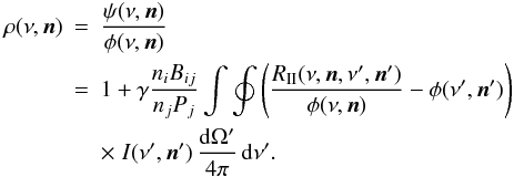$\begin{array}{ccc}\mathit{\rho }\mathrm{\left(}\mathit{\nu ,}{n}\mathrm{\right)}& \mathrm{=}& \frac{\mathit{\psi }\mathrm{\left(}\mathit{\nu ,}{n}\mathrm{\right)}}{\mathit{\phi }\mathrm{\left(}\mathit{\nu ,}{n}\mathrm{\right)}}\\ & \mathrm{=}& \mathrm{1}\mathrm{+}\mathit{\gamma }\frac{{\mathit{n}}_{\mathit{i}}{\mathit{B}}_{\mathit{ij}}}{{\mathit{n}}_{\mathit{j}}{\mathit{P}}_{\mathit{j}}}\mathrm{\int }\mathrm{􏽉}\left(\frac{{\mathit{R}}_{\mathrm{II}}\mathrm{\left(}\mathit{\nu ,}{n}\mathit{,}{\mathit{\nu }}^{\mathrm{\prime }}\mathit{,}{n}\mathrm{\prime }\mathrm{\right)}}{\mathit{\phi }\mathrm{\left(}\mathit{\nu ,}{n}\mathrm{\right)}}\mathrm{-}\mathit{\phi }\mathrm{\left(}{\mathit{\nu }}^{\mathrm{\prime }}\mathit{,}{n}\mathrm{\prime }\mathrm{\right)}\right)\\ & & \mathrm{\times }\mathit{I}\mathrm{\left(}{\mathit{\nu }}^{\mathrm{\prime }}\mathit{,}{n}\mathrm{\prime }\mathrm{\right)}\hspace{0.17em}\frac{\mathrm{d}{\mathrm{\Omega }}^{\mathrm{\prime }}}{\mathrm{4}\mathit{\pi }}\hspace{0.17em}\mathrm{d}{\mathit{\nu }}^{\mathrm{\prime }}\mathit{.}\end{array}$(1)Here, ν and ν′ are frequencies of the emitted and absorbed photon in the observer’s frame, n and n′ their respective directions, γ is the coherency fraction, n_i and n_j are the populations of the lower and upper level of the line, B_ij is the Einstein coefficient for radiative excitation and P_j is the total rate coefficient out of the upper level, R_II is the angle-dependent observer’s frame redistribution function for a broadened upper and a sharp lower level and I is the intensity.

The redistribution function is given by Hummer (1962) as $\begin{array}{ccc}{\mathit{R}}_{\mathrm{II}}\left(\mathit{q,}{n}\mathit{,}{\mathit{q}}^{\mathrm{\prime }}\mathit{,}{n}\mathrm{\prime }\right)& \mathrm{=}& \frac{\mathit{g}\mathrm{\left(}{n}\mathit{,}{{n}}^{\mathbf{\prime }}\mathrm{\right)}}{\mathrm{4}{\mathit{\pi }}^{\mathrm{2}}\sin \mathit{\gamma }}\exp \left[\mathrm{-}\left(\frac{\mathit{q}\mathrm{-}{\mathit{q}}^{\mathrm{\prime }}}{\mathrm{2}}\right){\csc }^{\mathrm{2}}\left(\frac{\mathit{\gamma }}{\mathrm{2}}\right)\right]\\ & & \mathrm{\times }\mathit{H}\left(\frac{\mathit{a}}{\mathrm{\Delta }{\mathit{\nu }}_{\mathrm{D}}}\sec \frac{\mathit{\gamma }}{\mathrm{2}}\mathit{,}\frac{\mathit{q}\mathrm{+}{\mathit{q}}^{\mathrm{\prime }}}{\mathrm{2}}\sec \frac{\mathit{\gamma }}{\mathrm{2}}\right)\mathrm{·}\end{array}$(2)Here g(n,n^′) is the dipole scattering phase function, $\mathit{g}\mathrm{\left(}{n}\mathit{,}{{n}}^{\mathbf{\prime }}\mathrm{\right)}\mathrm{=}\frac{\mathrm{3}}{\mathrm{16}\mathit{\pi }}\mathrm{(}\mathrm{1}\mathrm{+}{\cos }^{\mathrm{2}}{\mathit{\gamma }}^{\mathrm{)}}\mathit{,}$(3)${\mathit{q}}^{\mathrm{(}}{\mathrm{\prime }\mathrm{)}}^{}\mathrm{=}\mathrm{(}{\mathit{\nu }}^{\mathrm{(}}{\mathrm{\prime }\mathrm{)}}^{}\mathrm{-}{\mathit{\nu }}_{\mathrm{0}}\mathrm{)}\mathit{/}\mathrm{\Delta }{\mathit{\nu }}_{\mathrm{D}}$ are the reduced frequencies of the absorbed and emitted photon, with ν₀ and Δν_D the line center frequency and the Doppler width. The acute angle between n and n′ is given by γ, H is the Voigt function and a the line damping parameter.

Note that the second term in the integral of Eq. (1) is $\mathrm{\int }\mathrm{􏽉}\mathit{\phi }\mathrm{\left(}\mathit{\nu ,}{n}\mathrm{\right)}\mathit{I}\mathrm{\left(}\mathit{\nu ,}{n}\mathrm{\right)}\hspace{0.17em}\frac{\mathrm{d\Omega }}{\mathrm{4}\mathit{\pi }}\hspace{0.17em}\mathrm{d}\mathit{\nu }\mathrm{=}{\mathit{R}}_{\mathit{ij}}\mathit{/}{\mathit{B}}_{\mathit{ij}}\mathit{,}$(4)with R_ij the upward radiative rate coefficient that appears in the rate equations.

In a static atmosphere the absorption profile does not depend on direction. If one furthermore assumes that the radiation field is isotropic, i.e.,$\mathit{I}\mathrm{\left(}\mathit{\nu ,}{n}\mathrm{\right)}\mathrm{=}\frac{\mathrm{1}}{\mathrm{4}\mathit{\pi }}\mathrm{􏽉}\mathit{I}\mathrm{\left(}\mathit{\nu ,}{n}\mathrm{\right)}\hspace{0.17em}\mathrm{d\Omega }\mathrm{=}\mathit{J}\mathrm{\left(}\mathit{\nu }\mathrm{\right)}\mathit{,}$(5)then the angle integral in Eq. (1) can be performed analytically (see Hubený 1982) yielding a significantly simpler expression for the profile ratio: $\mathit{\rho }\mathrm{\left(}\mathit{\nu ,}{n}\mathrm{\right)}\mathrm{=}\mathrm{1}\mathrm{+}\mathit{\gamma }\frac{{\mathit{n}}_{\mathit{i}}{\mathit{B}}_{\mathit{ij}}}{{\mathit{n}}_{\mathit{j}}{\mathit{P}}_{\mathit{j}}}\mathrm{\int }\left({\mathit{g}}_{\mathrm{II}}\mathrm{(}\mathit{\nu ,}\hspace{0.17em}{\mathit{\nu }}^{\mathrm{\prime }}\mathrm{)}\mathrm{-}\mathit{\phi }\mathrm{\left(}{\mathit{\nu }}^{\mathrm{\prime }}\mathrm{\right)}\right)\mathit{J}\mathrm{\left(}{\mathit{\nu }}^{\mathrm{\prime }}\mathrm{\right)}\hspace{0.17em}\mathrm{d}{\mathit{\nu }}^{\mathrm{\prime }}\mathit{.}$(6)This simplification is often called angle-averaged PRD.

The function g_II can be computed efficiently using the approximation by Gouttebroze (1986) with the generalization to cross-redistribution by Uitenbroek (1989).

The assumption of an isotropic radiation field generally yields results very close to the full angle-dependent case for atmospheres without, or with only a weak, velocity field (Uitenbroek 2002).

However, Eq. (6) typically becomes inaccurate when the velocities in the atmosphere are larger than the Doppler velocity $\sqrt{\mathrm{2}\mathit{kT}\mathit{/}\mathit{m}}$ because Eq. (5) is no longer valid, and one should ideally use the angle-dependent formula (Eq. (1)). Unfortunately, using the angle-dependent expression is computationally expensive in both memory requirements and computing time. The computation of Eq. (1) is at least a factor n_a slower than the computation of Eq. (6), with n_a the number of rays used for the direction integration of the radiation field.

The way the angle-dependent MALI scheme is set up one needs to store the intensity I(ν,n) and the profile ratio ρ(ν,n) in memory, amounting to 2   n_ν   n_a floating point numbers per spatial grid point, in addition to all other quantities that need to be retained. Ideally one also stores the redistribution function R_II to avoid recomputation every iteration, which requires an additional ${\mathit{n}}_{\mathit{\nu }}^{\mathrm{2}}\hspace{0.17em}{\mathit{n}}_{\mathrm{a}}^{\mathrm{2}}$ floating point numbers per spatial grid point.

The memory and computing time requirements are easily met for a 1D model atmosphere. However, if one wants to compute synthetic line profiles from time series of 3D radiation-MHD models, a faster algorithm to compute the angle-dependent PRD profile ratio is desirable, if not required.

3. Hybrid PRD

The algorithm we propose should not be much slower than the angle-averaged case, yet capture the effects of velocities. It turns out that such a method is fairly simple:

The agreement between angle-dependent and angle-averaged PRD in static atmospheres implies that the angle-dependence caused by anisotropy of the radiation field is minor. Instead, the majority of the radiation anisotropy at a given wavelength experienced by a parcel of gas in the observer’s frame in a moving atmosphere is caused by sampling the line profile at different Doppler shifts when it receives radiation from different directions. If we first transform the radiation field to the rest frame of the moving gas parcel, we can again assume that the radiation field is isotropic. Then we can use Eq. (6) to compute the profile ratio in the rest frame, replacing the angle-averaged intensity in the observer’s frame J(ν) with the angle-averaged intensity in the parcel’s rest frame: $\begin{array}{ccc}& & {\mathit{\rho }}_{\mathrm{r}}\mathrm{\left(}{\mathit{\nu }}_{\mathrm{r}}\mathit{,}{n}\mathrm{\right)}\mathrm{=}\mathrm{1}\mathrm{+}\mathit{\gamma }\frac{{\mathit{n}}_{\mathit{i}}{\mathit{B}}_{\mathit{ij}}}{{\mathit{n}}_{\mathit{j}}{\mathit{P}}_{\mathit{j}}}\mathrm{\int }\left({\mathit{g}}_{\mathrm{II}}\mathrm{\left(}{\mathit{\nu }}_{\mathrm{r}}\mathit{,}\hspace{0.17em}{\mathit{\nu }}_{\mathrm{r}}^{\mathrm{\prime }}\mathrm{\right)}\mathrm{-}\mathit{\phi }\mathrm{\left(}{\mathit{\nu }}_{\mathrm{r}}^{\mathrm{\prime }}\mathrm{\right)}\right){\mathit{J}}_{\mathrm{r}}\mathrm{\left(}{\mathit{\nu }}_{\mathrm{r}}^{\mathrm{\prime }}\mathrm{\right)}\hspace{0.17em}\mathrm{d}{\mathit{\nu }}_{\mathrm{r}}^{\mathrm{\prime }}\mathit{.}\\ & & {\mathit{J}}_{\mathrm{r}}\mathrm{\left(}{\mathit{\nu }}_{\mathrm{r}}\mathrm{\right)}\mathrm{=}\frac{\mathrm{1}}{\mathrm{4}\mathit{\pi }}\mathrm{􏽉}\mathit{I}\mathrm{\left(}{\mathit{\nu }}_{\mathrm{r}}\mathrm{\right(}\mathrm{1}\mathrm{-}{n}\mathrm{·}{u}\mathit{/}\mathit{c}\mathrm{\left)}\mathit{,}{n}\mathrm{\right)}\hspace{0.17em}\mathrm{d\Omega }\mathit{.}\end{array}$\arraycolsep1.75ptThe quantity J_r(ν_r) can be computed incrementally from the observer’s frame intensity I(ν,n) during the standard angle-frequency integration needed to compute the radiative rate coefficients, without having to keep the intensity for each spatial location, frequency and angle in memory.

Plugging J_r(ν_r) into Eq. (6) instead of J(ν) yields a direction-independent emission to absorption ratio in the rest frame ρ_r(ν_r). Both J_r(ν_r) and ρ_r(ν_r) must be stored in memory, but as they are angle-independent they require a factor n_a less storage than the angle-dependent quantities I(ν,n) and ρ(ν,n). The MALI method requires ρ in the observer’s frame, which is accomplished through a frequency shift: $\mathit{\rho }\mathrm{\left(}\mathit{\nu ,}{n}\mathrm{\right)}\mathrm{=}{\mathit{\rho }}_{\mathrm{r}}\mathrm{\left(}{\mathit{\nu }}_{\mathrm{r}}\mathrm{\right(}\mathrm{1}\mathrm{+}{n}\mathrm{·}{u}\mathit{/}\mathit{c}\mathrm{\left)}\mathrm{\right)}\mathit{.}$(9)Numerically, this shift can be performed by a fast interpolation.

4. Results

Idealized test case.

To demonstrate the effect of the various methods to compute the profile ratio we performed an idealized test case computation.

As intensity we took the emergent intensity of the Ca II  H line computed from the standard FALC model atmosphere (Fontenla et al. 1990) with an artificially enhanced K2R peak to introduce an asymmetry in the line profile. We also introduced a directional anisotropy by setting $\mathit{I}\mathrm{\left(}{n}\mathrm{\right)}\mathrm{=}{\mathit{I}}_{\mathrm{e}}\left(\mathrm{1}\mathrm{-}\frac{\cos \mathit{\theta }}{\mathrm{2}}\right)$(10)with I_e the emergent intensity and θ the angle between the vertical and the direction n. These intensities are shown as grey curves in Fig. 1 as function of the reduced frequency q = (ν − ν₀)/Δν_D for different values of θ, where we assumed Δν_D = (ν₀/c) × 8 km s^-1. The black curve shows the angle-averaged intensity in the observer’s frame J. The red curve shows J_r, the angle-averaged intensity in the rest frame of a gas parcel moving with a velocity of (u_x,u_y,u_z) = (0,1,3) in units of the Doppler speed. The angle integrations were performed using the A8 set from Carlson (1963), which uses 10 rays per octant. The presence of the velocity smoothes the K2V and K2R peaks in the gas parcel’s rest frame. The K2R peak is reduced in height and has an increased width, the K3 minimum is smoothed out and the K2V peak is a barely discernible hump at q = 4.

Fig. 1 Plots of the radiation field used in the test computation as function of the reduced frequency q. Grey curves: intensity for different directions in the observer’s frame. Black curve: angle-averaged radiation field in the observer’s frame. Red curve: angle-averaged radiation field in the rest frame of a gas parcel moving with a velocity (ux,uy,uz) = (0,1,3) in units of the Doppler speed.

Fig. 2 Emission to absorption profile ratio computed using angle-dependent redistribution (black, Eq. (1)), angle-independent redistribution (blue, Eq. (6)) and our intermediate method (red, see Sect. 2) in the observer’s frame as function of reduced frequency q. The cosines of the angle of the ray direction with the coordinate axes (μx,μy,μz) are given in the upper left corner of the panel. The quantity α gives the angle between the gas velocity and the ray direction.

Figure 2 shows ρ(q) given the intensity and gas velocity described above for two different directions (given in the upper left corner of the panels). We assumed γ = 0.9 and n_iB_ij/(n_jP_j) = 5 × 10⁵. The black curve represents the angle-dependent case (AD-PRD, Eq. (1)), the blue curve the angle-averaged case (AA-PRD, Eq. (6)), while the red curve shows the hybrid case (H-PRD, Eq. (9)). The upper panel displays scattering into the direction of movement and shows a blue-shifted ρ-profile for the AD-PRD and H-PRD cases. The AA-PRD case does not take the gas velocity into account and is centered at q = 0. In AD-PRD and H-PRD the profile ratio has a fairly smooth lowest part, reflecting the smoothing of the radiation field in the rest frame. Compared to H-PRD, the AD-PRD profile ratio exhibits additional wiggles owing to the directional anisotropy of the radiation.

The lower panel shows scattering with an angle close to perpendicular to the velocity. As a consequence all ρ profiles are approximately centered around ρ = 0. Still the H-PRD case reproduces the true AD-PRD profile ratio much better than the AA-PRD formulation.

1D test atmospheres.

We implemented the hybrid method into the RH code by Uitenbroek (2001), which is also capable of using the angle-dependent and angle-independent redistribution function. We used this code to compute the emergent intensity from five 1D plane-parallel model atmospheres in non-LTE with the three recipes for PRD for a 4-level plus continuum Mg II and a 5-level plus continuum H I model atom. As model atmospheres we took columns from a snapshot of a 3D radiation-MHD simulation computed with the Bifrost code (Gudiksen et al. 2011). The details of this particular snapshot can be found in Leenaarts et al. (2012), but are not important here: the snapshot merely provides self-consistent model atmospheres with a velocity field. No microturbulence was added. We treated Mg II h & k, Lyα and Lyβ in PRD, all other lines were treated using complete redistribution. For the angle integration of the radiation field we used a ten-point Gauss-Legendre quadrature.

For all atmospheres and ray directions we found that the H-PRD method reproduces the true AD-PRD emergent line profile much more accurately than the AA-PRD method. We illustrate this in Fig. 3, which shows the emergent intensity for a near vertical ray (μ_z = 0.95) for the three different treatments of the redistribution function for two different model atmospheres.

Both atmospheres show a complex velocity and temperature structure (panels a and b). The second row (c and d) displays the emergent Mg II k intensity. For this line we expect strong angle-dependent PRD effects as the Doppler width of the line profile (2.6 km s^-1 at a temperature of 10 kK) is small compared to the flow velocities in the atmospheres. This is indeed the case, the AA-PRD profile (blue) is very different from the AD-PRD and H-PRD profiles. In panel c the former has a higher emission peak at the blue side of the line core, whereas the latter two have a higher peak on the red side. In panel d the AD-PRD and H-PRD profiles show a stronger emission peak on the red side of the line core.

The bottom row (e and f) compares the Lyα profiles. The effect of angle-dependent PRD is much smaller than for the Mg II k line because the Doppler width of the line profile (13 km s^-1 at a temperature of 10 kK) is larger than the typical atmospheric velocities.

Fig. 3 Comparison of PRD treatment in two plane-parallel model atmospheres (left-hand and right hand column respectively) taken from a radiation-MHD model. Panels a) and b) show the temperature (black) and vertical velocity structure (red) of the atmospheres. Panels c) and d) show the emergent intensity in the Mg II  k line, with PRD treated fully angle-dependent (black), angle-averaged (blue) and the hybrid approach (red). Panels e) and f) show a similar profile comparison, but now for the Lyα line of hydrogen. The stars and diamonds in panels a) and b) indicate the τ = 1 height for the wavelengths indicated in panels c)–f), with stars for the Mg II  k line and diamonds for Lyα.

Computational speed.

In Table 1 we compare the running time of the code for the three PRD methods for both model atoms in a 1D atmosphere with 225 spatial points (the atmosphere in panel a of Fig. 3). The quantities n_ν and ${\mathit{n}}_{\mathit{\nu }}^{\mathrm{PRD}}$ are the number of frequencies used, and the number of frequencies in the PRD lines, respectively. The quantity t_FS is the time to perform the formal solution for all frequencies and angles, including the computation of J_r in the H-PRD case; t_PR is the time to compute the profile ratios (Eqs. (1), (6) and (9)); t_MALI is the time to perform one full MALI iteration, including three PRD sub-iterations (see Uitenbroek 2001).

The time spent in the formal solution is slightly longer in the H-PRD case compared to the other methods. This is due to the interpolations required to compute Eqs. (8) and (9) numerically. The computing time of the AD-PRD method is mainly spent in the computation of the profile ratio. The computation of the profile ratio is several hundred times faster in the AA-PRD and H-PRD cases. The total time per MALI iteration for AD-PRD is a factor 130 (30) longer for the Mg II (H I) computation than in the corresponding AA-PRD computation. In contrast, the time per iteration for the H-PRD case is only  ≈ 10% larger than for AA-PRD.

5. Discussion and conclusions

We have presented a fast approximate method to compute the angle-dependent emission to absorption profile ratio needed to compute line profiles for which PRD effects are important. Line profiles computed with this method approximate the true profiles computed with full angle-dependent PRD very well.

Test computations show that the new hybrid method is 30 to 130 times faster than the angle-dependent PRD computation and only  ≈ 10% slower than the angle-averaged PRD method. This makes it possible to compute accurate line profiles from time-series of 3D radiation-MHD models for lines where angle-dependent PRD effects are important.

Acknowledgments

J.L. recognizes support from the Netherlands Organization for Scientific Research (NWO).

References

All Tables

All Figures

	Fig. 1 Plots of the radiation field used in the test computation as function of the reduced frequency q. Grey curves: intensity for different directions in the observer’s frame. Black curve: angle-averaged radiation field in the observer’s frame. Red curve: angle-averaged radiation field in the rest frame of a gas parcel moving with a velocity (ux,uy,uz) = (0,1,3) in units of the Doppler speed.
In the text

Fig. 2 Emission to absorption profile ratio computed using angle-dependent redistribution (black, Eq. (1)), angle-independent redistribution (blue, Eq. (6)) and our intermediate method (red, see Sect. 2) in the observer’s frame as function of reduced frequency q. The cosines of the angle of the ray direction with the coordinate axes (μx,μy,μz) are given in the upper left corner of the panel. The quantity α gives the angle between the gas velocity and the ray direction.

In the text

Fig. 3 Comparison of PRD treatment in two plane-parallel model atmospheres (left-hand and right hand column respectively) taken from a radiation-MHD model. Panels a) and b) show the temperature (black) and vertical velocity structure (red) of the atmospheres. Panels c) and d) show the emergent intensity in the Mg II  k line, with PRD treated fully angle-dependent (black), angle-averaged (blue) and the hybrid approach (red). Panels e) and f) show a similar profile comparison, but now for the Lyα line of hydrogen. The stars and diamonds in panels a) and b) indicate the τ = 1 height for the wavelengths indicated in panels c)–f), with stars for the Mg II  k line and diamonds for Lyα.

In the text

References

- Carlson, B. G. 1963, Meth. Comput. Phys., 1, 1 [NASA ADS] [Google Scholar]
- Fontenla, J. M., Avrett, E. H., & Loeser, R. 1990, ApJ, 355, 700 [NASA ADS] [CrossRef] [Google Scholar]
- Gouttebroze, P. 1986, A&A, 160, 195 [NASA ADS] [Google Scholar]
- Gudiksen, B. V., Carlsson, M., Hansteen, V. H., et al. 2011, A&A, 531, A154 [NASA ADS] [CrossRef] [EDP Sciences] [Google Scholar]
- Hubený, I. 1982, J. Quant. Spec. Radiat. Transf., 27, 593 [Google Scholar]
- Hummer, D. G. 1962, MNRAS, 125, 21 [NASA ADS] [CrossRef] [Google Scholar]
- Leenaarts, J., Carlsson, M., & Rouppe van der Voort, L. 2012, ApJ, 749, 136 [NASA ADS] [CrossRef] [EDP Sciences] [Google Scholar]
- Rybicki, G. B., & Hummer, D. G. 1991, A&A, 245, 171 [NASA ADS] [Google Scholar]
- Rybicki, G. B., & Hummer, D. G. 1992, A&A, 262, 209 [NASA ADS] [Google Scholar]
- Uitenbroek, H. 1989, A&A, 216, 310 [NASA ADS] [Google Scholar]
- Uitenbroek, H. 2001, ApJ, 557, 389 [NASA ADS] [CrossRef] [Google Scholar]
- Uitenbroek, H. 2002, ApJ, 565, 1312 [NASA ADS] [CrossRef] [Google Scholar]