| Issue |
A&A
Volume 543, July 2012
|
|
|---|---|---|
| Article Number | A16 | |
| Number of page(s) | 8 | |
| Section | Numerical methods and codes | |
| DOI | https://doi.org/10.1051/0004-6361/201219028 | |
| Published online | 21 June 2012 | |
Adaptable radiative transfer innovations for submillimetre telescopes (ARTIST)
Dust polarisation module (DustPol)
1 Institut de Ciències de l’Espai (CSIC–IEEC), Campus UAB, Facultat de Ciències, Torre C5p, 08193 Bellaterra, Catalunya, Spain
e-mail: This email address is being protected from spambots. You need JavaScript enabled to view it.
; This email address is being protected from spambots. You need JavaScript enabled to view it.
; This email address is being protected from spambots. You need JavaScript enabled to view it.
2 Centre for Star and Planet Formation and Niels Bohr Institute, University of Copenhagen, Juliane Maries Vej 30, 2100 Copenhagen Ø., Denmark
e-mail: This email address is being protected from spambots. You need JavaScript enabled to view it.
; This email address is being protected from spambots. You need JavaScript enabled to view it.
3 Laboratoire de radioastronomie, UMR 8112 du CNRS, École normale supérieure et Observatoire de Paris, 24 rue Lhomond, 75231 Paris Cedex 05, France
e-mail: This email address is being protected from spambots. You need JavaScript enabled to view it.
4 Jet Propulsion Laboratory, 4800 Oak Grove Drive, Pasadena, CA 91109, USA
e-mail: This email address is being protected from spambots. You need JavaScript enabled to view it.
5 Department of Earth and Space Sciences, Chalmers University of Technology, Onsala Space Observatory, 439 92 Onsala, Sweden
e-mail: This email address is being protected from spambots. You need JavaScript enabled to view it.
6 Argenlander Institute for Astronomy, University of Bonn, Auf dem Hügel 71, 53121 Bonn, Germany
e-mail: This email address is being protected from spambots. You need JavaScript enabled to view it.
; This email address is being protected from spambots. You need JavaScript enabled to view it.
7 Leiden Observatory, Leiden University, PO Box 9513, 2300 RA Leiden, The Netherlands
e-mail: This email address is being protected from spambots. You need JavaScript enabled to view it.
; This email address is being protected from spambots. You need JavaScript enabled to view it.
Received: 13 February 2012
Accepted: 28 April 2012
Abstract
We present a new publicly available tool (DustPol) aimed to model the polarised thermal dust emission. The module DustPol, which is publicly available, is part of the ARTIST (Adaptable Radiative Transfer Innovations for Submillimetre Telescopes) package, which also offers tools for modelling the polarisation of line emission together with a model library and a Python-based user interface. DustPol can easily manage analytical as well as pre-gridded models to generate synthetic maps of the Stokes I, Q, and U parameters. These maps are stored in FITS format which is straightforwardly read by the data reduction software used, e.g., by the Atacama Large Millimeter Array (ALMA). This turns DustPol into a powerful engine for the prediction of the expected polarisation features of a source observed with ALMA or the Planck satellite as well as for the interpretation of existing submillimetre observations obtained with other telescopes. DustPol allows the parameterisation of the maximum degree of polarisation and we find that, in a prestellar core, if there is depolarisation, this effect should happen at densities of 106 cm-3 or larger. We compare a model generated by DustPol with the observational polarisation data of the low-mass Class 0 object NGC 1333 IRAS 4A, finding that the total and the polarised emission are consistent.
Key words: radiative transfer / methods: numerical / polarization / submillimeter: general
© ESO, 2012
1. Introduction
The importance of magnetic fields in regulating the physics of star formation is still a matter of debate. The main schools of thought invoke either the leakage of magnetic support through ambipolar diffusion (Mestel & Spitzer 1956) or the supersonic turbulence which compresses the gas at the interfaces between converging flows (Elmegreen 1993). While turbulent energy is required to sustain a cloud over its lifetime (Gammie & Ostriker 1996), ohmic dissipation time of magnetic fields is much larger than the collapse time, assuming a typical ionisation fraction of ~ 10-8–10-7 and density of ~105 cm-3 (Pinto & Galli 2008). Collapse time scale for a subcritical core is a few million to 107 yr assuming the ambipolar diffusion to be the dominant process (Mouschovias et al. 2006). Conversely, if collapse is controlled by turbulence, the time scale is shorter, of the order of 106 yr (Mac Low & Klessen 2004). Cores can also be forced into collapse because of external events such as collision between clouds as well as supernova shock waves with a time scale as short as 105 yr (Boss et al. 2010). All these different mechanisms most likely take part in cloud collapse, but the role of magnetic fields cannot be ruled out from star formation theories, even when a core is supercritical (Basu 1997).
From an observational point of view, it is possible to gather information about the strength and the geometry of magnetic fields through measurements of the Zeeman splitting of hyperfine molecular transitions as well as measurements of polarisation of thermal dust emission in the (sub)millimetre wavelength range. Observations of the Zeeman effect provide information about the line of sight component of the magnetic field and have been carried out using atoms and molecules which show large magnetic moments (e.g. Crutcher et al. 1996; Falgarone et al. 2008). By observing maser emission it is possible to detect both circular and linear polarisation, making it possible to derive the full 3D magnetic field (Vlemmings et al. 2011; Surcis et al. 2011a,b). On the other hand, polarisation of the thermal dust emission probes the plane of the sky component of magnetic fields, providing information about the field geometry in molecular clouds and filaments associated with star formation regions (e.g. Novak et al. 1989; Matthews et al. 2001; 2002; Davidson et al. 2011). (Sub)Millimetre wavelength interferometric observations, first with the Berkeley-Illinois-Maryland Association array, BIMA (e.g. Girart et al. 1999; Lai et al. 2003), and nowadays with the Submillimeter Array, SMA (Girart et al. 2009; Rao et al. 2009; Tang et al. 2009) have proven useful to study the magnetic field properties at high angular resolution, probing scales of a few hundreds AU at which the dynamical collapse of the star forming cores is occurring.
The Atacama Large Millimeter Array (ALMA) is the largest interferometer and the largest ground based project in (sub)millimetre astronomy. It provides a considerable enhancement in resolution, sensitivity and imaging with respect to previous interferometers operating at these wavelengths. Since dust and a multitude of spectral lines can be observed at the same time, ALMA allows an in-depth investigation of the physical and chemical properties of e.g. embedded protostars, zooming in to AU scales of nearby star-forming regions. ALMA will also open new possibilities for studying magnetic fields. In fact, due to the receiver capabilities, full polarisation calibration and imaging will be the norm rather than the exception. For these reasons, providing ALMA users with self-consistent tools for polarisation modelling will be very important. The publicly available Adaptable Radiative Transfer Innovations for Submillimetre Telescopes1 (ARTIST) package (Jørgensen et al., in prep.) provides a direct link between the theoretical predictions and the quantitative constraints from the submillimetre observations, being able to model the full multi-dimensional structure of, e.g., a low-mass protostar, including its envelope, disk, outflow, and magnetic field.
The model suite is based on LIME2 (Line Modelling Engine, Brinch & Hogerheijde 2010), a non-LTE radiative transfer code using adaptive gridding in three dimensions that allows simulations of sources with arbitrary multi-dimensional structures ensuring a rapid convergence. In addition, ARTIST offers unique tools for modelling the polarisation of dust and line emission and an extensive library of theoretical (semi-analytical) models. All these packages are connected by a comprehensive Python-based graphical user interface with direct link to, e.g., ALMA data reduction software (Common Astronomy Software Applications package, CASA3).
In this paper, we describe the dust polarisation module of ARTIST: in Sect. 2 we briefly describe the polarisation of stellar radiation due to dust grains, in Sect. 3 we explain the features of the module for analysing dust polarisation emission, and in Sect. 4 we demonstrate the capabilities of the routines to handle analytical models, numerical simulations, and providing a comparison to observations. Finally, in Sect. 5 we summarise our results and conclusions.
2. Origin of dust polarisation
Dust grain alignment provides a natural explanation for the origin of polarisation in the ISM. However, what mechanisms are responsible for grain alignment and what role they play in different environments remain poorly understood (Lazarian 2003, 2007). The main explanations are supplied by paramagnetic (Davis & Greenstein 1951) and mechanical alignment (Gold 1951), but other mechanisms have been proposed as well (Martin 1971; Purcell 1979; Draine & Weingartner 1996). Recent studies for example show that radiative torques, which are the results of the interaction of irregular grains with a flow of photons, can effectively align the dust grains (Dolginov & Mytrophanov 1976; Lazarian 2007).
Grains are most likely non-spherical since they are formed by stochastic growth processes leading to irregular shapes (Fogel & Leung 1998). Unpolarised starlight passing through an aligned-grain set will acquire polarisation due to the different grain extinction parallel and perpendicular to the alignment direction, since they absorb more light along their longer direction. This depends on the fact that extinctions are proportional to the parallel and perpendicular grain cross section (see Lee & Draine 1985; and Efroimsky 2002, for a detailed discussion for spheroidal grains and a more general case, respectively).
Conversely, in the submillimetre wavelength regime, the electric-field vector of the thermal continuum emission emerging from rotating aligned grains has its maximum value in the plane containing the longer grain axis. The partially linearly polarised vectors are parallel to the mean grain orientation, therefore perpendicular to the magnetic field as projected on the plane of the sky. Consequently, from the observation of the polarised dust emission it is possible to model the morphology of magnetic fields in the plane of the sky, the degree of polarisation depending on various contributions as the grain cross sections, the temperature, the composition, and the density.
3. Dust polarisation tools
With the dust polarisation module (DustPol) of ARTIST we aim to model the polarised dust continuum emission. The DustPol module is an extension to the LIME radiative transfer code. LIME is a non-LTE molecular excitation and line radiation transfer code that is mainly used to calculate line profiles in the far-infrared and submillimetre regimes. However, LIME can also ray-trace given density and temperature profiles and from that estimate the emerging continuum flux. It is this feature that we make use of in the DustPol module presented in this paper. At the relatively long wavelengths at which LIME operates, scattering is negligible and therefore the problem of making an image of the continuum model is reduced to integrating the source function  (1)along lines of sight through the model. Bλ(Tdust) is the Planck function evaluated at the dust temperature Tdust and dτλ = κλ ρdust ds, where κλ is the wavelength dependent dust opacity and ρdust is the dust mass density. The main benefit of using the LIME code for our application is its ability to automatically map a 3D model onto a computational grid. The grid points are placed at random in 3D space with probability of a point being placed at a given location weighted by a user-selected function, typically the underlying model dust density distribution. This results in a higher spatial grid point density in high dust density regions and vice versa for low density regions, which means that the expectation distance between neighbour points scales with the photon mean free path.
Once the grid points have been placed, the Voronoi diagram of the distribution and the topological equivalent, the Delaunay triangulation, is calculated (Ritzerveld & Icke 2006). A Voronoi region associated with a certain grid point is defined as the set containing points that is located closer to the generating grid point than to any other grid point. The result is a tessellation of space consisting of random polyhedra. All physical properties are taken to be constant over each polyhedra (or Voronoi cell). If the model resolution turns out insufficient in specific regions, more grid points can be added to these and the Voronoi diagram is recalculated. The grid is then regularised by moving each grid point slightly toward the centroid of the corresponding Voronoi cell several times in an iterative process. The result is a random grid consisting of approximately regular polyhedra (see Brinch & Hogerheijde 2010, for details). Ray-tracing is done by integrating straight lines of sight (rays) through the grid simply by summing up the constant contribution between the two intersections between a ray and the Voronoi facets for each Voronoi cell the ray passes through.
For the dust polarisation calculations, the main extension to LIME is to include Stokes Q and U in the source function. We followed the procedure developed by Lee & Draine (1985), then by Wardle & Königl (1990), Fiege & Pudritz (2000), and Padoan et al. (2001). As in Gonçalves et al. (2005) and Frau et al. (2011), hereafter GGW05 and FGG11, respectively, our code accounts for the dependence of the emerging continuum radiation on dust temperature distribution (Tdust) supplied by the user (e.g., calculated self-consistently through tools such as RADMC/RADMC-3D4; Dullemond & Dominik 2004). According to this method, the polarisation degree p and the polarisation (or position) angle χ, that is the direction of polarisation in the plane of the sky, are given by  (2)and
  (3)respectively. q, u, and i are called “reduced” Stokes parameters and are defined in terms of the standard Stokes parameters through a constant which depends on the cross section, a polarisation reduction factor due to imperfect grain alignment and to the turbulent component of the magnetic field, and the Planck function. The “reduced” parameters are described by
 ![Mathematical equation: \begin{eqnarray} q&=&\int_{0}^{\infty}\alpha_{\rm max}\ B_\lambda(T_{\rm dust})\ {\rm e}^{-\tau_\lambda}\,\cos2\psi\,\cos^{2}\gamma\,\ud\tau_\lambda, \\[2mm] u&=&\int_{0}^{\infty}\alpha_{\rm max}\ B_\lambda(T_{\rm dust})\ {\rm e}^{-\tau_\lambda}\,\sin2\psi\,\cos^{2}\gamma\,\ud\tau_\lambda, \end{eqnarray}](/articles/aa/full_html/2012/07/aa19028-12/aa19028-12-eq26.png) and
and  (6)where ψ is the angle between the north direction in the plane of the sky and the component of the magnetic field (B) in this plane and γ is the angle between the direction of B and the plane of the sky. Σ and Σ2 are given by
  (7)and
  (8)where αmax accounts for grain cross sections and alignment properties. For polarised grains, the effective cross section is given by the difference between the extinction cross section and a contribution coming from polarisation. For grains without polarisation properties, Stokes I is basically given by Σ. Indeed, the grain properties may vary with density (Fiege & Pudritz 2000), but in the absence of detailed information, unless otherwise specified, we assume αmax to be constant and equal to 0.15 in the remainder of this paper, corresponding to a maximum polarisation degree of about 15%, as suggested by GGW05. Higher values has not been observed and lower values appear unable to reproduce observations of the magnetic field of prestellar cores (FGG11). However, it is important to notice that the DustPol module allows the maximum polarisation degree to vary according to a user defined function (e.g. density or temperature dependent).
After the ray-tracing, the code creates a file in FITS format which consists of three slices, one for each Stokes parameters. This FITS file can be read by the sim_observe-sim_analyze tasks in the CASA package to prefigure the expected polarised flux intensity map obtained by ALMA.
4. Applications
In this Section, a few applications of the DustPol routines are presented, showing their capabilities to manage input from analytical models as well as numerical simulations. A comparison with SMA available observations is also provided.
4.1. Toy models
It is instructive to start by considering geometrical models to check the effective accuracy of the code. We examine sources with a purely toroidal (Btor), a dipole (Bdip), and a quadrupole (Bquad) magnetic field whose spherical components (Br,Bθ,Bφ) are ![Mathematical equation: \begin{eqnarray} {\vec B}_{\rm tor}&\propto&(0,0,r^{-1}), \\[2mm] {\vec B}_{\rm dip}&\propto& \left(-\frac{2\cos\theta}{r^3},-\frac{\sqrt{1-\cos^2\theta}}{r^3},0\right), \end{eqnarray}](/articles/aa/full_html/2012/07/aa19028-12/aa19028-12-eq40.png) and
and  (11)respectively. We assumed a Bonnor-Ebert sphere (BES) density profile (Bonnor 1956; Ebert 1955) with a central density of 2 × 10¹³ m-3, a radius of the inner flat region of 500 AU, and an outer radius of 0.1 pc. We adopted a wavelength of 850 μm, a constant dust temperature equal to 10 K for a source at the distance of 140 pc, and a resolution of
  . Images have then been smoothed to a beam of 10′′ to get sharper contours. The magnetic field configurations are shown for four different inclinations with respect to the plane of the sky, from zero (face-on source) to π/2 radians (edge-on source).
Figure 1 refers to a purely toroidal magnetic field. As expected, for a face-on source field lines are concentric while, approaching to the edge-on configuration, they become parallel in the plane of the sky and can be pictured as concentric rings perpendicular to the vertical axis of symmetry of the source. It can be easily understood that the depolarisation in the outer parts is due to the bending of the field lines which become perpendicular to the line of sight.
Figures 2 and 3 show a radial configuration of the polarisation vectors for a face-on source as well as the expected dipole and quadrupole field shape arising as the inclination increases.
 |
Fig. 1 Polarisation maps for a purely toroidal magnetic field and a BES density distribution (model radius, rmodel = 2.25 × 10⁴ AU). Black vectors represent the direction of the magnetic field, whose length is proportional to the fractional polarisation, obtained by flipping by 90 degrees the dust polarisation vectors. White contours show 50 and 90 per cent of the 850-μm dust emission (Stokes I) peak and the coloured map depicts the polarised flux intensity (Ip). The scale bar to the right gives Ip in Jy/(10′′ beam). The inclination of the models with respect to the plane of the sky is given in the upper left corner of each subplot. The synthesised beam is shown in the lower left corner. |
 |
Fig. 2 Polarisation maps for a dipole magnetic field and a BES density distribution (rmodel = 2.25 × 10⁴ AU). See Fig. 1 for further information. |
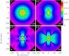 |
Fig. 3 Polarisation maps for a quadrupole magnetic field and BES density distribution (rmodel = 2.25 × 10⁴ AU). See Fig. 1 for further information. |
 |
Fig. 4 Polarisation maps for the H0 = 1.25 singular isothermal toroid according to the LS96 model (rmodel = 2.8 × 10³ AU). White contours show 10, 30, 50, 70, and 90 per cent of the 850-μm dust emission (Stokes I) peak and the scale bar to the right gives the polarised flux intensity in Jy/(1′′ beam). See Fig. 1 for further information. |
4.2. Analytical models
In order to test the correctness of our code, we reproduced the model described in Li & Shu (1996), hereafter LS96, to compare our results with those obtained by GGW05. This detailed comparison of the LS96 model between the results of GGW05 and our code is worthwhile to have a further validation of the reliability of the code. The model of LS96 is a semi-analytical, self-similar description of an axi-symmetric isothermal, self-gravitating protostellar core. It reproduces the hourglass magnetic field configuration suggested by observations (Girart et al. 2006). The governing equations hinge on a dimension-less parameter, H0, which characterises the fraction of support provided against self-gravity by poloidal magnetic fields relative to that of gas pressure (see LS96 for more details). In particular, Fig. 4 shows the results for a core with H0 = 1.25, observed at 850 μm. We adopted a distance of 140 pc, Tdust = 10 K and an angular resolution of  . Images have been smoothed to 1′′ for plotting.
Our computation supports the conclusions of GGW05 concerning the depolarisation at intermediate inclinations. In the central regions the bending of the field lines is stronger and the integration along line of sights close to the centre leads to a lower polarisation degree. We compared the minimum and the maximum degree of polarisation as a function of the inclination of the core with values computed by GGW05. For a direct comparison, we smoothed our model results to 12′′ which is the beam used in GGW05 and we obtain a substantial agreement as shown in Fig. 5.
 |
Fig. 5 Maximum (solid lines) and mininum (dotted lines) percentage of polarisation degree as a function of the inclination of the core with respect to the plane of the sky. DustPol model, solid squares; GGW05 model, empty squares. |
 |
Fig. 6 Degree of polarisation (p) as a function of the intensity normalised to its peak value (I/Imax) for the LS96 toroid with an inclination of 50 degrees with respect to the plane of the sky for different wavelengths, temperatures, and values of H0. Each point in these diagrams represents a grid point from the model and multiple tracks are an artefact due to the grid sampling. The red dashed lines show the maximum and minimum values of the polarisation degree found by GGW05, see their Fig. 8. Regions on the right of the vertical blue solid lines correspond to the extent of the polarisation holes. |
We examined the dependence of the polarisation degree on wavelength, temperature, and H0, finding analogies with GGW05. The two top panels of Fig. 6 show the dependence of the polarisation degree on the wavelength. Due to the fact that the emission for lower wavelengths is rather flat and less concentrated (Gonçalves et al. 2004), the region with low and uniform values of p, the so-called polarisation hole, has a smaller extent in this figure at 450 μm with respect to 850 μm. It follows that, if the polarisation hole has a fixed physical radius, the corresponding value of I/Imax will be larger at 450 μm than at 850 μm. We also probed the dependence of the polarisation degree on the dust temperature as shown by the comparison of the two left panels of Fig. 6. The lower left panel shows the result for the assumption of an external heating with Tdust going from ~15 to ~8 K inside a radius of 0.1 pc (Gonçalves et al. 2004). As in GGW05, we conclude that a non-isothermal distribution of the dust temperature may help the observation of the depolarisation effect. In fact, the magnetic field component in the plane of the sky is generally larger far from the central thermal dust emission peak. Thus, when in presence of an interstellar radiation field, the contribution of the external layers of the prestellar core to the Stokes parameters becomes substantial. Finally, we examined the dependence of the polarisation degree on H0, which is altering the magnetic field support. The lower right panel of Fig. 6 shows the distribution of the polarisation degree for H0 = 0.125, corresponding to a mild pinching of the magnetic field lines. As found in GGW05, it is interesting to notice that even a low value of H0 leads to modifications of the polarisation degree for increasing intensities, measured as the difference between the maximum (pmax) and the minimum (pmin) degree of polarisation observed. For H0 = 0.125, we found Δp = pmax − pmin = 4.5% while, for comparison, Δp = 7.6% for H0 = 1.25, that is for a more pinched field, assuming in both cases ν = 850 μm, Tdust = 10 K, and αmax = 15%.
The magnetic field geometry and temperature distribution are important components for the description of the observed values of the polarisation degree, but they cannot account for the whole set of observational constraints. For example, it is known that the maximum degree of polarisation, αmax, is strongly dependent on the cutoff in the grain size distribution (Cho & Lazarian 2005) and depolarisation may be the result of alterations in the grain structure at higher densities which may reduce the dust grain alignment efficiency (Lazarian & Hoang 2007). In order to test the dependence of the polarisation on grain properties, we assumed a step function for αmax, which drops from 15% to zero for molecular hydrogen number densities higher than 105, 106, 107, and 108 cm-3. Results are shown in Fig. 7. As expected, the polarisation degree decreases with intensity more rapidly as the limit on n(H2) decreases. Despite the assumption of the step function is purely arbitrary, it is possible to deduce that the case of no polarisation for n(H2) > 105 cm-3 has to be discarded since there is no observational evidence that p is zero for I ≳ 0.2Imax. Although the theory of grain alignment is still not completely developed, the extreme flexibility in the parameterisation of αmax allows the user to easily explore the parameter space.
 |
Fig. 7 Degree of polarisation (p) as a function of the intensity normalised to its peak value (I/Imax) for the LS96 toroid as in Fig. 6. This plot shows the decrease in p for high values of I/Imax due to the assumption of a step function for the maximum degree of polarisation. Labels (105 to 108 cm-3) represent the limit on n(H2) above which αmax = 0. |
4.3. Numerical models
The novelty of DustPol is that it can easily manage inputs from numerical simulations set out on regular or irregular grids. In this paper we give a couple of examples of 3D numerical calculations of a collapsing magnetised dense core (Hennebelle & Fromang 2008; Hennebelle & Ciardi 2009) which make use of the adaptive mesh refinement (AMR) code RAMSES (Teyssier 2002; Fromang et al. 2006). We describe only qualitatively the results postponing quantitative conclusions for a following paper (Padovani et al., in prep.).
The grid of a numerical simulation is sampled as if it were an analytic function. Each point of the grid built by LIME takes the value of density, temperature, and magnetic field of the closest model point. Before this step, the output of a numerical simulation has to be converted in the format readable by LIME. To this end, a simple wrapper is distributed together with DustPol.
RAMSES was run for a collapsing rotating core with mass-to-flux ratio equal to 5. The magnetic field and the angular momentum vectors are initially aligned. We extracted four snapshots from the RAMSES run at four times (see caption of Fig. 8), chosen in order to predict the evolution of the polarisation since magnetic field lines get tangled as the core rotates. The output of the RAMSES run at these time samples was used as input to DustPol using a distance of 140 pc, with a wavelength of 850 μm, Tdust = 10 K, and an angular resolution of  , then smoothed at , which is a resolution typically achievable by ALMA. Note that these maps are not corrected for the instrumental response of the interferometer. Initially, the magnetic field has hourglass shape, as time increases, the field configuration becomes purely toroidal. Figure 8 shows the time evolution for a face-on configuration, which yields an initially radial pattern changing to a more toroidal structure.
 |
Fig. 8 Polarisation maps for a collapsing magnetised dense core (face-on view) obtained with the RAMSES code (rmodel = 6.3 × 10² AU). Labels refer to different times of the collapse: t1 = 1.76 × 10⁴ yr, t2 = 1.86 × 10⁴ yr, t3 = 1.94 × 10⁴ yr, and t4 = 2.96 × 10⁴ yr. White contours show 30, 50, 70, and 90 per cent of the 850-μm dust emission (Stokes I) peak and the scale bar to the right gives Ip in Jy/( |
Finally, we tested DustPol using a large scale RAMSES simulation (Dib et al. 2010) relative to a prestellar core with a mass of 1.62 M⊙, which has been obtained from the “Molecular cloud evolution with decaying turbulence” project of the StarFormat database5. The upper panel of Fig. 9 shows the column density distribution of molecular hydrogen, N(H2), of this core. DustPol has been used to get the polarisation pattern using a distance of 140 pc, Tdust = 10 K, and a wavelength of 850 μm. The resulting image is shown in the lower panel of Fig. 9. It has been smoothed from 1′′ to  which is the beam of SCUBA, accounting for the error beams for an accurate description of the beam profile (Hogerheijde & Sandell 2000).
Under the optically thin assumption, the agreement between the RAMSES H2 column density distribution and the DustPol Stokes I map is remarkable. In fact, after normalising N(H2) and Stokes I with respect to their maximum values, we computed the ratio between N(H2) and Stokes I finding a mean value of 0.95 ± 0.12. Additionally, it is worth noting the displacement between the polarised emission and the dust continuum emission near the offset (0,0) and, conversely, the good overlap near ( − 100,150). This can be easily understood by looking at the local direction of the magnetic field into the RAMSES data cube. We found that the magnetic field points towards the line of sight around the centre of the map, thus explaining the decrease in polarisation degree. On the other hand, the direction of the magnetic field mainly lays on the plane of the sky near the north-west clump, where the polarisation is stronger.
Working in tandem, DustPol and StarFormat (to be publicly available) can be used to interpret large-scale polarisation maps of molecular clouds, investigating on magnetic field morphologies.
 |
Fig. 9 Upper panel: column density distribution of molecular hydrogen for a prestellar core extracted from the StarFormat database. Black and white contours show 30, 50, 70, and 95 per cent of the H2 column density peak and of the 850-μm dust emission (Stokes I) peak, respectively. The scale bar to the right gives N(H2) in logarithmic scale. Lower panel: polarisation map for the core depicted in the upper panel (rmodel = 2.8 × 10⁴ AU). The scale bar to the right gives Ip in Jy/( |
 |
Fig. 10 Top panel: dust polarisation SMA maps toward NGC 1333 IRAS 4A from FGG11. Middle panel: synthetic dust polarisation map generated with DustPol, following the FGG11 convolution scheme, using the best fitting parameters of the Allen et al. (2003) model found by FGG11 (see Sect. 4.4 for more details). Each panel shows the intensity (contours), polarised intensity (pixel map), and direction of magnetic field (blue segments). Contours depict emission levels from 6σ up to the maximum value in steps of 6σ, where σ = 0.02 Jy beam-1. The middle panel shows the beam and the angular and spatial scale. Bottom panel: histogram of the difference between the position angles computed with the radiative transfer tool in FGG11 and DustPol. |
4.4. Comparison with observations: NGC 1333 IRAS 4A
The ultimate goal of the DustPol project is to generate simulations capable of being compared to the real data. Its main advantage is that it provides quick convergence because of the adaptive gridding and it easily accommodates outputs from other codes as shown in Sects. 4.2 and 4.3. Recently, FGG11 have developed a method to compare the observational polarisation maps of the low-mass Class 0 object NGC 1333 IRAS 4A to a set of magnetohydrodynamic (MHD) simulations, which allows to find the best set of models that fit the magnetic field properties of NGC 1333 IRAS 4A. They generate a synthetic source based on models and simulations and, using the same equation set described in this work, they provide synthetic Stokes maps. These synthetic maps are convolved by the interferometric response in order to obtain the spatially filtered maps comparable to the real data. To assess the quality of the DustPol module, we repeated this scheme replacing the radiative transfer tool in FGG11 with DustPol. We used the Allen et al. (2003) model datacube with the best fitting parameters found by FGG11, namely a mass of 1.6 M⊙, a mean volume density within the angular size of 100 AU of 3 × 108 cm-3, an inclination of 45 degrees with respect to the plane of the sky, H0 = 0.125 (see Sect. 4.2), and the dust temperature profile derived by Maret et al. (2002). We ran DustPol with a resolution of  , assuming a source distance of 300 pc, and a wavelength of 880 μm. Then, we applied the same convolution tool developed first by Gonçalves et al. (2008) and improved by FGG11 to the output map of DustPol for a final synthesised beam of
  . Figure 10 shows our results, to be compared with the third row of Fig. 8 in FGG11. The observations and the model are in good agreement and the general morphologies of the total emission (Stokes I) and the polarised emission are consistent. In fact, even if the polarisation vectors in the map generated by DustPol cover a larger area, the difference map between the Stokes Q (and U) maps created by the two radiative transfer tools show no features above the 3σ level (σ = 2.5 mJy beam-1). Therefore, the differences are due to the statistical noise at the low RMS regions. Finally, the differences between the position angles evaluated with the radiative transfer tool in FGG11 and DustPol have a standard deviation of 0.48 degrees, confirming the reliability of DustPol.
5. Conclusions
We have presented the DustPol module of the Adaptable Radiative Transfer Innovations for Submillimetre Telescopes (ARTIST) package, a tool for modelling the polarisation of thermal dust emission self-consistently. The module is an extension to the radiative transfer code LIME making it possible to model complex three-dimensional structures. The synergy between DustPol and codes such as RAMSES and RADMC-3D will help to enlighten the interpretation of the role of magnetic fields in star-forming regions.
DustPol can easily handle analytical as well as pre-gridded models and outputs from other codes, accounting for the dependence on dust temperature and, for the first time to our knowledge, for variations of the polarisation degree. A number of examples (Sect. 4) demonstrate the capabilities and the accuracy of DustPol to interpret existing submillimetre data as well as new data from ALMA and the Planck satellite. The output of DustPol is a FITS file whose header is consistent with the format of the input models for the sim_observe-sim_analyze tasks of the CASA package. This makes it straightforward, e.g., to make prediction about the polarised flux for a given configuration of the ALMA antennas.
The code is publicly available as long as appropriate reference is made to this paper. It is accessible through the complete ARTIST package, taking advantage of the Python-based graphic user interface that includes a model library or through a stand-alone version.
Acknowledgments
M.P. would like to acknowledge Daniele Galli for many helpful and inspiring discussions on development of the code and on drafting the paper. We also want to thank the referee, Karl Misselt, for careful reading of the manuscript and helpful comments. This work was funded as part of the ASTRONET initiative by the Spanish (MINECO), Dutch (NWO), and German (BMBF) funding agencies. M.P., J.M.G. and P.F. are supported by MINECO grants AYA2008-04451-E, AYA2008-06189-C03-02, and AYA2011-30228-C03-02 (Spain) and by AGAUR grant 2009SGR1172 (Catalonia). P.F. is partially supported by MINECO fellowship FPU (Spain). The research in Copenhagen is supported by a Junior Group Leader Fellowship from the Lundbeck Foundation to J.K.J. as well as by the Danish National Research Foundation through the establishment of Centre for Star and Planet Formation. Part of the time, R.K. is financially supported by grant “LPDS 2011-5” of the Leopoldina Fellowship Programme. W.V. acknowledges support by the Deutsche Forschungsgemeinschaft (DFG; through the Emmy Noether Research grant VL 61/3-1).
References
- Allen, A., Shu, F. H., & Li, Z. 2003, ApJ, 599, 351 [NASA ADS] [CrossRef] [Google Scholar]
- Basu, S. 1997, ApJ, 485, 240 [CrossRef] [Google Scholar]
- Bonnor, W. B. 1956, MNRAS, 116, 351 [CrossRef] [Google Scholar]
- Boss, A. P., Keiser, S. A., Ipatov, S. I., Myhill, E. A., & Vanhala, H. A. T. 2010, ApJ, 708, 1268 [NASA ADS] [CrossRef] [Google Scholar]
- Brinch, C., & Hogerheijde, M. 2010, A&A, 523, A25 [NASA ADS] [CrossRef] [EDP Sciences] [Google Scholar]
- Cho, J., & Lazarian, A. 2005, ApJ, 631, 361 [NASA ADS] [CrossRef] [Google Scholar]
- Crutcher, R. M., Troland, T. H., Lazareff, B., & Kazès, I. 1996, ApJ, 456, 217 [NASA ADS] [CrossRef] [Google Scholar]
- Davidson, J. A., Novak, G., Matthews, T. G., et al. 2011, ApJ, 732, 97 [NASA ADS] [CrossRef] [Google Scholar]
- Davis, L., & Greenstein, J. L. 1951, ApJ, 114, 206 [Google Scholar]
- Dib, S., Hennebelle, P., Pineda, J. E., et al. 2010, ApJ, 723, 425 [NASA ADS] [CrossRef] [Google Scholar]
- Dolginov, A. Z., & Mytrophanov, I. G. 1976, Ap&SS, 43, 257 [NASA ADS] [CrossRef] [Google Scholar]
- Draine, B. T., & Weingartner, J. C. 1996, ApJ, 470, 551 [NASA ADS] [CrossRef] [Google Scholar]
- Dullemond, C. P., & Dominik, C. 2004, A&A, 417, 159 [NASA ADS] [CrossRef] [EDP Sciences] [Google Scholar]
- Ebert, R. 1955, Z. Astron., 37, 217 [Google Scholar]
- Efroimsky, M. 2002, ApJ, 575, 886 [NASA ADS] [CrossRef] [Google Scholar]
- Elmegreen, B. G. 1993, ApJ, 419, L29 [NASA ADS] [CrossRef] [Google Scholar]
- Falgarone, E., Troland, T. H., Crutcher, R. M., & Paubert, G. 2008, A&A, 487, 247 [NASA ADS] [CrossRef] [EDP Sciences] [Google Scholar]
- Fiege, J. D., & Pudritz, R. E. 2000, ApJ, 544, 830 [NASA ADS] [CrossRef] [Google Scholar]
- Fogel, M. E., & Leung, C. M. 1998, ApJ, 501, 175 [NASA ADS] [CrossRef] [Google Scholar]
- Frau, P., Galli, D., & Girart, J. M. 2011, A&A, 535, A44 (FGG11) [NASA ADS] [CrossRef] [EDP Sciences] [Google Scholar]
- Fromang, S., Hennebelle, P., & Teyssier, R. 2006, A&A, 457, 371 [NASA ADS] [CrossRef] [EDP Sciences] [Google Scholar]
- Gammie, C. F., & Ostriker, E. C. 1996, ApJ, 466, 814 [NASA ADS] [CrossRef] [Google Scholar]
- Girart, J. M., Crutcher, R. M., & Rao, R. 1999, ApJ, 525, L109 [NASA ADS] [CrossRef] [Google Scholar]
- Girart, J. M., Rao, R., & Marrone, D. P. 2006, Science, 313, 812 [NASA ADS] [CrossRef] [PubMed] [Google Scholar]
- Girart, J. M., Beltrán, N., Zhang, Q., Rao, R., & Estalella, R. 2009, Science, 324, 1408 [NASA ADS] [CrossRef] [PubMed] [Google Scholar]
- Gold, T. 1951, Nature, 169, 322 [Google Scholar]
- Gonçalves, J., Galli, D., & Walmsley, C. M. 2004, A&A, 415, 617 [NASA ADS] [CrossRef] [EDP Sciences] [Google Scholar]
- Gonçalves, J., Galli, D., & Walmsley, C. M. 2005, A&A, 430, 979 (GGW05) [NASA ADS] [CrossRef] [EDP Sciences] [Google Scholar]
- Gonçalves, J., Galli, D., & Girart, J. M. 2008, A&A, 490, L39 [NASA ADS] [CrossRef] [EDP Sciences] [Google Scholar]
- Hennebelle, P., & Fromang, S. 2008, A&A, 477, 9 [NASA ADS] [CrossRef] [EDP Sciences] [Google Scholar]
- Hennebelle, P., & Ciardi, A. 2009, A&A, 506, L29 [NASA ADS] [CrossRef] [EDP Sciences] [Google Scholar]
- Hogerheijde, M., & Sandell, G. 2000, ApJ, 534, 880 [NASA ADS] [CrossRef] [Google Scholar]
- Lai, S.-P., Girart, J. M., & Crutcher, R. M. 2003, ApJ, 598, 392 [NASA ADS] [CrossRef] [Google Scholar]
- Lazarian, A. 2003, J. Quant. Spectr. Rad. Trans., 79, 881 [Google Scholar]
- Lazarian, A. 2007, J. Quant. Spectr. Rad. Trans., 106, 225 [NASA ADS] [CrossRef] [Google Scholar]
- Lazarian, A., & Hoang, T. 2007, MNRAS, 378, 910 [Google Scholar]
- Lee, H. M., & Draine, B. T. 1985, ApJ, 290, 211 [NASA ADS] [CrossRef] [Google Scholar]
- Li, Z.-Y., & Shu, F. H. 1996, ApJ, 472, 211 (LS96) [NASA ADS] [CrossRef] [Google Scholar]
- Mac Low, M.-M., & Klessen, R. S. 2004, RvMP, 76, 125 [Google Scholar]
- Maret, S., Ceccarelli, C., Caux, E., Tielens, A. G. G. M., & Castets, A. 2002, A&A, 395, 573 [NASA ADS] [CrossRef] [EDP Sciences] [Google Scholar]
- Martin, P. G. 1971, MNRAS, 153, 279 [NASA ADS] [Google Scholar]
- Matthews, B. C., & Wilson, C. D. 2002, ApJ, 574, 822 [NASA ADS] [CrossRef] [Google Scholar]
- Matthews, B. C., Wilson, C. D., & Fiege, J. D. 2001, ApJ, 562, 400 [NASA ADS] [CrossRef] [Google Scholar]
- Mestel, L., & Spitzer, L. 1956, MNRAS, 116, 503 [NASA ADS] [CrossRef] [Google Scholar]
- Mouschovias, T. C., Tassis, K., & Kunz, M. W. 2006, ApJ, 646, 1043 [NASA ADS] [CrossRef] [Google Scholar]
- Novak, G., Gonatas, D. P., Hildebrand, R. H., Platt, S. R., & Dragovan, M. 1989, ApJ, 345, 802 [NASA ADS] [CrossRef] [Google Scholar]
- Padoan, P., Goodman, A., Draine, B. T., et al. 2001, ApJ, 559, 1005 [NASA ADS] [CrossRef] [Google Scholar]
- Pinto, C., & Galli, D. 2008, A&A, 484, 17 [NASA ADS] [CrossRef] [EDP Sciences] [Google Scholar]
- Purcell, E. M. 1979, ApJ, 231, 404 [NASA ADS] [CrossRef] [Google Scholar]
- Rao, R., Girart, J. M., Marrone, D. P., Lai, S.-P., & Schnee, S. 2009, ApJ, 707, 921 [NASA ADS] [CrossRef] [Google Scholar]
- Ritzerveld, J., & Icke, V. 2006, Phys. Rev. E, 74, 26704 [Google Scholar]
- Surcis, G., Vlemmings, W. H. T., Curiel, S., et al. 2011a, A&A, 527, A48 [NASA ADS] [CrossRef] [EDP Sciences] [Google Scholar]
- Surcis, G., Vlemmings, W. H. T., Torres, R. M., van Langevelde, H. J., & Hutawarakorn Kramer, B. 2011b, A&A, 533, A47 [NASA ADS] [CrossRef] [EDP Sciences] [Google Scholar]
- Tang, Y.-W., Ho, P. T. P., Koch, P. M., et al. 2009, ApJ, 700, 251 [NASA ADS] [CrossRef] [Google Scholar]
- Teyssier, R. 2002, A&A, 385, 337 [NASA ADS] [CrossRef] [EDP Sciences] [Google Scholar]
- Vlemmings, W. H. T., Humphreys, E. M. L., & Franco-Hernández, R. 2011, ApJ, 728, 149 [NASA ADS] [CrossRef] [Google Scholar]
- Wardle, M., & Königl, A. 1990, ApJ, 362, 120 [NASA ADS] [CrossRef] [Google Scholar]
All Figures
|
Fig. 1 Polarisation maps for a purely toroidal magnetic field and a BES density distribution (model radius, rmodel = 2.25 × 10⁴ AU). Black vectors represent the direction of the magnetic field, whose length is proportional to the fractional polarisation, obtained by flipping by 90 degrees the dust polarisation vectors. White contours show 50 and 90 per cent of the 850-μm dust emission (Stokes I) peak and the coloured map depicts the polarised flux intensity (Ip). The scale bar to the right gives Ip in Jy/(10′′ beam). The inclination of the models with respect to the plane of the sky is given in the upper left corner of each subplot. The synthesised beam is shown in the lower left corner. |
| In the text | |
|
Fig. 2 Polarisation maps for a dipole magnetic field and a BES density distribution (rmodel = 2.25 × 10⁴ AU). See Fig. 1 for further information. |
| In the text | |
|
Fig. 3 Polarisation maps for a quadrupole magnetic field and BES density distribution (rmodel = 2.25 × 10⁴ AU). See Fig. 1 for further information. |
| In the text | |
|
Fig. 4 Polarisation maps for the H0 = 1.25 singular isothermal toroid according to the LS96 model (rmodel = 2.8 × 10³ AU). White contours show 10, 30, 50, 70, and 90 per cent of the 850-μm dust emission (Stokes I) peak and the scale bar to the right gives the polarised flux intensity in Jy/(1′′ beam). See Fig. 1 for further information. |
| In the text | |
|
Fig. 5 Maximum (solid lines) and mininum (dotted lines) percentage of polarisation degree as a function of the inclination of the core with respect to the plane of the sky. DustPol model, solid squares; GGW05 model, empty squares. |
| In the text | |
|
Fig. 6 Degree of polarisation (p) as a function of the intensity normalised to its peak value (I/Imax) for the LS96 toroid with an inclination of 50 degrees with respect to the plane of the sky for different wavelengths, temperatures, and values of H0. Each point in these diagrams represents a grid point from the model and multiple tracks are an artefact due to the grid sampling. The red dashed lines show the maximum and minimum values of the polarisation degree found by GGW05, see their Fig. 8. Regions on the right of the vertical blue solid lines correspond to the extent of the polarisation holes. |
| In the text | |
|
Fig. 7 Degree of polarisation (p) as a function of the intensity normalised to its peak value (I/Imax) for the LS96 toroid as in Fig. 6. This plot shows the decrease in p for high values of I/Imax due to the assumption of a step function for the maximum degree of polarisation. Labels (105 to 108 cm-3) represent the limit on n(H2) above which αmax = 0. |
| In the text | |
|
Fig. 8 Polarisation maps for a collapsing magnetised dense core (face-on view) obtained with the RAMSES code (rmodel = 6.3 × 10² AU). Labels refer to different times of the collapse: t1 = 1.76 × 10⁴ yr, t2 = 1.86 × 10⁴ yr, t3 = 1.94 × 10⁴ yr, and t4 = 2.96 × 10⁴ yr. White contours show 30, 50, 70, and 90 per cent of the 850-μm dust emission (Stokes I) peak and the scale bar to the right gives Ip in Jy/( |
| In the text | |
|
Fig. 9 Upper panel: column density distribution of molecular hydrogen for a prestellar core extracted from the StarFormat database. Black and white contours show 30, 50, 70, and 95 per cent of the H2 column density peak and of the 850-μm dust emission (Stokes I) peak, respectively. The scale bar to the right gives N(H2) in logarithmic scale. Lower panel: polarisation map for the core depicted in the upper panel (rmodel = 2.8 × 10⁴ AU). The scale bar to the right gives Ip in Jy/( |
| In the text | |
|
Fig. 10 Top panel: dust polarisation SMA maps toward NGC 1333 IRAS 4A from FGG11. Middle panel: synthetic dust polarisation map generated with DustPol, following the FGG11 convolution scheme, using the best fitting parameters of the Allen et al. (2003) model found by FGG11 (see Sect. 4.4 for more details). Each panel shows the intensity (contours), polarised intensity (pixel map), and direction of magnetic field (blue segments). Contours depict emission levels from 6σ up to the maximum value in steps of 6σ, where σ = 0.02 Jy beam-1. The middle panel shows the beam and the angular and spatial scale. Bottom panel: histogram of the difference between the position angles computed with the radiative transfer tool in FGG11 and DustPol. |
| In the text | |
Current usage metrics show cumulative count of Article Views (full-text article views including HTML views, PDF and ePub downloads, according to the available data) and Abstracts Views on Vision4Press platform.
Data correspond to usage on the plateform after 2015. The current usage metrics is available 48-96 hours after online publication and is updated daily on week days.
Initial download of the metrics may take a while.