© ESO, 2012

1. Introduction

The interstellar medium (ISM) is composed of gas and dust, where the dust component represents about 1% of the total ISM mass. Interstellar gas provides the material for star formation, making it a central part in the life cycle of matter. The gas is either atomic, molecular, or ionized and these three phases are commonly observed using the HI 21 cm emission, CO transitions, and either H_α or free-free emission, respectively. Several studies have reported an emission excess in the far-infrared (FIR) with respect to the gas, that is correlated with none of the gas tracers. These excess detections were first obtained for Galactic regions (Reach et al. 1994; Meyerdierks & Heithausen 1996). By analyzing the diffuse γ-ray emission from the ISM, Grenier et al. (2005) concluded that there is an additional gas phase in our Galaxy called “dark gas” (DG), which has a non-negligible mass. This component has also been discovered in the Magellanic clouds (Leroy et al. 2007; Bernard et al. 2008; Roman-Duval et al. 2010).

The Planck Collaboration (2011a) obtained all-sky maps of the dust optical depth and, comparing it with the observed gas column density, constructed a map of the DG distribution covering a large fraction of the intermediate Galactic latitude sky ( | b |  > 10°). On average, they estimated that the mass of DG is 28% of the atomic mass and 118% of the molecular gas traced by CO emission in the solar neighborhood. These results indicate that the DG is detected at intermediate hydrogen column densities, corresponding to extinctions values between 0.4 and 2.5 mag. The first possible explanation is that the DG could be molecular gas, which is not detected using the CO(J = 1–0) transition. It is indeed expected that a layer of pure H₂ or dissociated CO should exist around dense clouds (e.g. Wolfire et al. 2010) that would be undetectable because at temperatures below 100 K (which is typical of these environments), the fluxes from the H₂ rotational transitions are too low. However, this layer could also be traced using other species such as C⁺ (see Langer et al. 2010). Other possible origins were suggested by the Planck Collaboration (2011a) to explain the observed departure from linearity between the dust optical depth (τ) and the observable gas column density, namely: (1) variations in the dust/gas ratio (D/G), (2) weak CO emission undetected at the sensitivity of the CO survey, (3) optically thin approximation for the HI emission not valid over the entire sky, and (4) formation of dust aggregates, inducing a higher dust emissivity. For hypothesis (1), the authors concluded that variations in D/G of about 30% are unlikely in the solar neighborhood. Assumptions (2) and (3) were tested by performing the analysis with an upper limit in the weak CO emission in one case, and with a different HI spin temperature in the other case. The authors deduced that these two effects could not account for the whole excess. The last option (4) can be tested using extinction data, since dust aggregates are expected to have a higher FIR emissivity than isolated grains, but mostly unaffected optical properties in the visible and ultra-violet. Therefore, no substantial A_V excess relative to the gas column density should be observed in that case. We note that γ-ray observations would not detect any excess if the FIR excess were due to either D/G or dust optical property variations.

The large dust particles that emit in the FIR are also responsible for the main extinction in the visible and near-infrared (NIR). Extinction data are therefore well-suited to checking for the presence of DG. An extinction map covering the whole sky was produced by Dobashi (2011) using the Two Micron All Sky Survey Point Source Catalog (2MASS PSC). This map has since been significantly improved to correct for the background-star intrinsic colors (Dobashi et al. 2012).

This study is carried out following the methodology adopted by Planck Collaboration (2011a), but using extinction instead of FIR optical depth. The use of dust optical depth requires us to determine dust temperature and therefore make assumptions about the dust emissivity shape and/or mixing effects along the line-of-sight (LOS). On the other hand, in principle, extinction directly measures dust column density. In practice however, large-scale extinction maps derived from star counts have limited accuracy and suffer from a bias inherent to the stars being intermixed with the gas, and starlight does not sample the whole LOS. In this analysis, we use the same gas tracers as in Planck Collaboration (2011a), so that the results can be compared directly.

Here, we compare the spatial distribution of the DG seen in absorption and emission, as well as the DG masses derived from the two approaches. We also wish to investigate whether the transition between the HI and H₂ phases is consistent with that found using FIR emission. In addition, we are interested in comparing our results with theoretical models such as that of Wolfire et al. (2010).

In Sect. 2, we present the dataset used in this analysis, in Sect. 3.1 we then describe the method we applied to perform the correlations between extinction data and gas tracers. We discuss the results in Sect. 4. Finally, a summary of our findings is provided in Sect. 5.

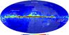Fig. 1 Extinction map (AV) in mag. Regions in light blue are not covered by the combination of the Dame et al. (2001) and NANTEN CO surveys, and are not used in our analyses. The red boxes correspond to individual regions defined in Sect. 3.1.3.

2. Observations

2.1. Extinction data

We used color excess maps produced by Dobashi (2011) based on the 2MASS PSC (Skrutskie et al. 2006). The maps were derived using a technique named “the X percentile method” (Dobashi et al. 2008, 2009), which is an extension of the well-known NICE method introduced by Lada et al. (1994). While the standard NICE method uses the mean color of stars found in a cell set on the sky to measure the color excess by dust, the X percentile method utilizes the X percentile reddest star (X = 100% is the reddest) and is unaffected by the contamination of unreddened foreground stars.

The combination of the maps of the Galactic plane and both north and south high Galactic latitudes cover the whole sky with a 1′ grid and a varying angular resolution (from 1′ to 12′) because of the “adaptive grid” mapping technique used (Cambrésy 1999). This technique adjusts the resolution to ensure a constant number of stars in the cells while measuring the color excess, and maintain a flat noise level all over the sky.

Among the color excess maps presented by Dobashi (2011), we chose to compare the E(J − H) map measured in the range 50 < X < 95% (based on his Eq. (4)) with the gas data, because this map is relatively more sensitive than other maps and has fewer defects in the regions studied in this paper ( | b |  > 10°). However, we note that the results obtained in the following do not change significantly when using other maps computed at different X values or from the other color excess available, E(H − K_S).

Here, we should note that there is a slight but systematic offset in the original color excess maps of Dobashi (2011); this arises from the rather ambiguous determination of the background star colors, i.e., the mean star colors unreddened by dust, which is needed to determine the zero point of the color excess. In general, when deriving a color excess map on large scales using the NICE method, it is virtually impossible to determine the background star colors precisely from the observed stars themselves, because the mean intrinsic star colors should vary on the sky and there is no region without dust across the Galactic plane. For simplicity, Dobashi (2011) assumed a constant mean intrinsic star color in all directions, as for other all-sky color excess maps derived in a similar way, e.g., by Rowles & Froebrich (2009); this led to a systematic offset in the final color excess map.

This varying offset is generally not large, but can cause significant problems when attempting to detect DG. To reduce these offsets, we use the new color-excess maps of Dobashi et al. (2012), who provided a correction to the original color-excess maps of Dobashi (2011) by determining the mean intrinsic star colors as a function of Galactic coordinates using the Besançon Galactic model (Robin et al. 2003), which is one of the latest Galactic stellar population synthesis model. On the basis of this model, they generated a star catalog equivalent to the 2 MASS PSC, but free from any interstellar dust, and calculated how the mean intrinsic star colors vary across the sky when applying the X percentile method to the simulated star catalog. They regarded the resulting star color maps as the background for the color-excess maps derived from the 2MASS PSC.

In addition, Dobashi et al. (2012) estimated the fraction of total dust along the LOS that escapes detection by the X percentile method, by simulating the effect of a diffuse dust disk on the simulated star catalog. The method is known to underestimate the diffuse dust component extending over a large region along the LOS, but it can retrieve extinction from individual well-defined dark clouds more precisely (Dobashi et al. 2009). As a result, they found that more than 80% of the total dust along the LOS should be detected in the Galactic latitude range  | b |  ≳ 5°, though the effect is more severe in the lower Galactic latitude range (e.g., by  ~ 50% at  | b |  ≃ 0°). They derived a map of the detection rate of the dust disk, which can be used to correct the color excess maps for this underestimation on large scales.

The color excess maps used in this work were corrected for the background star colors as well as for the underestimation of the diffuse and extended dust component. However, the corrected maps might still be erroneous close to  | b |  ≃ 0°, especially around the Galactic center, because of the inhomogeneous detection limits in the 2MASS PSC and/or unknown stellar populations not taken into account in the Besançon Model. Therefore, when we compare the maps with the gas data in the following, we restrict ourselves to  | b |  > 10°, where these corrections for the background and the underestimation are minimized. This also corresponds to the region studied in Planck Collaboration (2011a).

Finally, we converted the E(J − H) map to A_V using ${\mathit{A}}_{\mathrm{V}}\mathrm{=}\mathrm{10.9}\mathit{E}\mathrm{(}\mathit{J}\mathrm{-}\mathit{H}\mathrm{)}\mathit{,}$(1)where the coefficient corresponds to the empirical reddening law of Cardelli et al. (1989) for R_V = 3.1. The resulting map (see Fig. 1) has an almost constant noise level of ΔA_V ≃ 0.5 mag.

2.2. Gas tracers

The gas tracers used in this analysis are the same as described in Planck Collaboration (2011a). Here we provide a summary of the atomic (21 cm HI emission) and molecular (¹²CO(J = 1–0) line) surveys. We used the LAB (Leiden/Argentine/Bonn) survey to trace the atomic gas. This survey is a combination of the Leiden/Dwingeloo survey by Hartmann & Burton (1997) with sky observations above  − 30° of Galactic latitude (at a 36′ angular resolution), and the IAR (Instituto Argentino de Radioastronomia) survey (Arnal et al. 2000; Bajaja et al. 2005) of the Southern sky at latitudes below  − 25° (at a 30′ angular resolution). The LAB data were integrated in the velocity range  − 400 < V_LSR < 400 km s^-1. Assuming that the gas is optically thin, we deduced the hydrogen column density from the integrated intensity of the HI emission (W_HI) using ${\mathit{N}}_{\mathrm{HI}}\mathrm{=}{\mathit{X}}_{\mathrm{HI}}{\mathit{W}}_{\mathrm{HI}}\mathit{,}$(2)where X_HI is the HI integrated intensity to column-density conversion factor. This factor is taken to be equal to 1.82 × 10¹⁸ H/cm²/(K km s^-1) (Spitzer 1978).

For the molecular gas, we used the combination of three ¹²CO(J = 1–0) line surveys:

• the Dame et al. (2001) survey, in theGalactic plane, obtained with both the CfA telescope in the north(at an angular resolution of 8.4′) and CfA-Chile telescope in thesouth (at an angular resolution of 8.8′). The integrated intensitymap was derived by integrating the velocity range where the COemission is significantly detected (Dame 2011);

• the unpublished high latitude survey obtained with the CfA telescope, still observing the northern sky (Dame et al., in prep.). The data cube was integrated over 10–20 velocity channels;

• the NANTEN survey obtained from Chile for the intermediate Galactic latitudes not covered by the Dame et al. (2001) survey, at a 2.6′ angular resolution. This survey is still unpublished, but a full description of the NANTEN telescope can be found for instance in Fukui et al. (1999). The total intensity map was obtained by integrating the data cube over the whole velocity range.

Each survey was smoothed to a common resolution of 8.8′ using the convolution by a Gaussian kernel. As quoted in Planck Collaboration (2011a), the NANTEN data appear to have 24% higher values than those obtained with the CfA telescopes. This discrepancy is still poorly understood and following Planck Collaboration (2011a), the NANTEN data were decreased by 24%, before merging with the CfA survey, to bring them to the absolute scale of Dame et al. (2001). The total map used in this analysis is shown in Planck Collaboration (2011a), Fig. 1. The CO integrated intensity (W_CO) to column density conversion factor is derived from the relation ${\mathit{N}}_{{\mathrm{H}}_{\mathrm{2}}}\mathrm{=}{\mathit{X}}_{\mathrm{CO}}{\mathit{W}}_{\mathrm{CO}}\mathit{.}$(3)The value of the CO conversion factor (X_CO) is still debated. This factor is also expected to vary over the sky. For this reason, we made no assumption and derived X_CO instead from correlations (see Sect. 3.1).

The contribution of emission in the ionized medium is neglected in this study. This assumption is reasonable since we do not consider the Galactic plane emission, which includes most of the ionized medium emission caused by HII regions. However, its possible small contribution at high latitudes, which is correlated neither with atomic nor molecular-traced gas, can be accounted for in the constant term (${\mathit{A}}_{\mathrm{V}}^{\mathrm{0}}$) when performing the correlations (see Eq. (4)).

This work is done at the resolution of the HI data, i.e. 36′. All data are projected using the HEALPix pixelization scheme (Hierarchical Equal Area isoLatitude Pixelization)¹ with nside = 256, corresponding to a pixel size of 13.7′. The description of the projection method used is given in Appendix A.

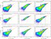Fig. 2 Correlation plots between extinction data (AV) and the total gas-column density (${\mathit{N}}_{\mathrm{H}}\mathrm{=}{\mathit{N}}_{\mathrm{H}}^{\mathrm{HI}}\mathrm{+}\mathrm{2}{\mathit{X}}_{\mathrm{CO}}{\mathit{W}}_{\mathrm{CO}}$) excluding the Galactic plane ( | b |  > 10°): high latitude sky (top panels), inner Galaxy (middle panels) and outer Galaxy (bottom panels). Left, middle, and right panels correspond respectively, to regions where no DG is detected (“no DG”) according to Planck Collaboration (2011a), where strong DG is detected (“DG”), and the entire region (“All”) (see Sect. 3.1). The color scale represents the density of pixels on a log scale. The yellow dots show the correlation binned in NH. The red lines show the best-fit linear correlation, constrained for the whole data in the “no DG” region. The short-dashed and long-dashed lines indicate the position of a departure from a linear fit, and the position where the correlation recovers a linear behavior, respectively.

3. Extinction/gas correlation

3.1. (A_V/N_H)^ref and X_CO determination

In Planck Collaboration (2011a), the reference value of the ratio of the dust optical depth to the gas column densities ($\mathrm{(}\frac{\mathit{\tau }}{{\mathit{N}}_{\mathrm{H}}}{\mathrm{)}}^{\mathrm{ref}}$) was determined from the correlation between τ and the gas tracers at low gas-column density. We followed the same type of analysis, and modeled the extinction $\mathrm{\left(}{\mathit{A}}_{\mathrm{V}}^{\mathrm{mod}}\mathrm{\right)}$ in the portion of the sky covered by the infrared, atomic, and CO-traced surveys, for  | b |  > 10°, as 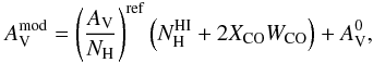${\mathit{A}}_{\mathrm{V}}^{\mathrm{mod}}\mathrm{=}{\left(\frac{{\mathit{A}}_{\mathrm{V}}}{{\mathit{N}}_{\mathrm{H}}}\right)}^{\mathrm{ref}}\mathrm{(}{\mathit{N}}_{\mathrm{H}}^{\mathrm{HI}}\mathrm{+}\mathrm{2}{\mathit{X}}_{\mathrm{CO}}{\mathit{W}}_{\mathrm{CO}}\mathrm{)}\mathrm{+}{\mathit{A}}_{\mathrm{V}}^{\mathrm{0}}\mathit{,}$(4)where ${{}^{\mathrm{\right(}}\frac{{\mathit{A}}_{\mathrm{V}}}{{\mathit{N}}_{\mathrm{H}}}^{\mathrm{\left)}}}^{\mathrm{ref}}$ is the reference value of the ratio of visible extinction to gas column density, and ${\mathit{A}}_{\mathrm{V}}^{\mathrm{0}}$ is a constant, which can account for ionized gas and/or the offset in the extinction map.

However, the A_V map is particularly noisy at low column density, which makes the estimate of ${{}^{\mathrm{\right(}}\frac{{\mathit{A}}_{\mathrm{V}}}{{\mathit{N}}_{\mathrm{H}}}^{\mathrm{\left)}}}^{\mathrm{ref}}$ difficult. We therefore adopted a slightly different approach from Planck Collaboration (2011a). Our analysis was done in two steps. We first selected regions with a limited amount of DG by identifying regions in Fig. 8 of Planck Collaboration (2011a) with DG column densities ${\mathit{N}}_{\mathrm{H}}^{\mathrm{X}}$ such that ${\mathit{N}}_{\mathrm{H}}^{\mathrm{X}}\mathit{/}{\mathit{N}}_{\mathrm{H}}\mathit{<}\mathrm{0.05}$ and we also imposed a low CO content (W_CO < 0.2 K km s^-1). For this region, which we refer to as “no DG”, we derived the best-fit parameters $\mathrm{(}\frac{{\mathit{A}}_{\mathrm{V}}}{{\mathit{N}}_{\mathrm{H}}}{\mathrm{)}}^{\mathrm{ref}}$ and ${\mathit{A}}_{\mathrm{V}}^{\mathrm{0}}$ using Eq. (4), but did not attempt to derive X_CO in this first step because the considered regions have little CO emission. Second, we repeated the same analysis including all pixels of the considered region included in the gas surveys (we refered to this region as “all”), while imposing the ${{}^{\mathrm{\right(}}\frac{{\mathit{A}}_{\mathrm{V}}}{{\mathit{N}}_{\mathrm{H}}}^{\mathrm{\left)}}}^{\mathrm{ref}}$ and ${\mathit{A}}_{\mathrm{V}}^{\mathrm{0}}$ values derived in the first step and determined the best-fit value for X_CO. We also computed the mass of DG from the difference between the best correlation and the data at that stage. The procedure above was applied to both the whole high Galactic latitude sky (see Sect. 3.1.1) and a set of individual regions (see Sect. 3.1.3), and in all cases was restricted to  | b |  > 10°.

Results of the correlations are presented in Table 1. The best-fit parameters were obtained from χ² minimization. Parameter uncertainties were derived from the difference between the minimum and maximum values of the parameters contained in interval Δχ², corresponding to a confidence level of 68%. We note that, for the purpose of illustrating the A_V-gas correlations (see Figs. 2 and 3), we also carried the correlation in a region with ${\mathit{N}}_{\mathrm{H}}^{\mathrm{X}}\mathit{/}{\mathit{N}}_{\mathrm{H}}\mathit{>}\mathrm{0.05}$, which we refered to as the “DG” region.

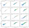Fig. 3 Correlation plots between extinction data (AV) and the total gas column density (${\mathit{N}}_{\mathrm{H}}\mathrm{=}{\mathit{N}}_{\mathrm{H}}^{\mathrm{HI}}\mathrm{+}\mathrm{2}{\mathit{X}}_{\mathrm{CO}}{\mathit{W}}_{\mathrm{CO}}$) in various regions excluding the Galactic plane ( | b |  > 10°), from top to bottom the Cepheus-Polaris, Taurus, Orion, and Aquila-Ophiuchus regions. Left, middle, and right panels correspond respectively, to regions where no DG is detected (“no DG”) according to Planck Collaboration (2011a), where strong DG is detected (“DG”), and the entire region (“All”) (see Sect. 3.1). The color scale represents the density of pixels on a log scale. The description of the yellow dots, red, and dashed lines is given in the caption of Fig. 2.

3.1.1. High Galactic latitude regions (|b| > 10°)

The correlation was first established across the whole high Galactic latitude sky ( | b |  > 10°) characterizing the solar neighborhood. Results are displayed in Fig. 2 (top panels). We note that the linear fits (slope = ${{}^{\mathrm{\right(}}\frac{{\mathit{A}}_{\mathrm{V}}}{{\mathit{N}}_{\mathrm{H}}}^{\mathrm{\left)}}}^{\mathrm{ref}}$) shown in the figures (red lines) were constrained using the whole data in the “no DG” region, and not the binned version of the data shown by yellow dots. The corresponding lines are curved as plotted on a log-log scale, because of the constant term. The investigation of this “no DG” region leads to an (A_V/N_H)^ref ratio of 6.53 × 10^-22 mag cm². This value is close to the reference value of 5.34 × 10^-22 obtained by Bohlin et al. (1978), which is relevant to the solar neighborhood and the Galactic plane. We found that the optimal X_CO is close to 1.67 × 10²⁰ H₂ cm^-2/(K km s^-1). This value is lower than the findings of Planck Collaboration (2011a), who derived an averaged X_CO = 2.54 × 10²⁰ H₂ cm^-2/(K km s^-1), but in better agreement with the Galactic average of 1.9 × 10²⁰ H₂ cm^-2/(K km s^-1) (Strong & Mattox 1996) and the value of 1.8 × 10²⁰ H₂ cm^-2/(K km s^-1) derived by Dame et al. (2001) for  | b |  > 5°.

Looking at Fig. 2, one can discern a different behavior in the A_V versus N_H plots (with ${\mathit{N}}_{\mathrm{H}}\mathrm{=}{\mathit{N}}_{\mathrm{H}}^{\mathrm{HI}}\mathrm{+}\mathrm{2}{\mathit{X}}_{\mathrm{CO}}{\mathit{W}}_{\mathrm{CO}}$), when comparing the “DG” and “no DG” regions at intermediate and high A_V. In the first case, looking at the binned data points the correlation shows an excess between N_H ≃ 4 × 10²⁰ cm^-2 (A_V = 0.2 mag) and N_H ≃ 3 × 10²¹ cm^-2 (A_V = 1.5 mag) compared to a linear fit, whereas we do not in the second case. We note that, owing to the low signal-to-noise ratio of the extinction data at low column densities, the location of these transitions were determined by eye here, while they were inferred from a fit in Planck Collaboration (2011a). These results imply that there is an additional gas phase, with a spatial distribution that is similar to that determined using the Planck data (Planck Collaboration 2011a). For comparison, these authors estimated that the excess appears at A_V ranging from 0.4 to 2.5 mag. However, results obtained by Planck Collaboration (2011b), by analyzing the diffuse ISM and Galactic halo, revealed some residual emission in the infrared/HI correlation, between N_H ≃ 3 × 10²⁰ cm^-2 (A_V ≃ 0.15 mag) and N_H ≃ 4 × 10²¹ cm^-2 (A_V ≃ 2.0 mag). Our results are in-between these two findings based on Planck data.

The column density of the dark component (${\mathit{N}}_{\mathrm{H}}^{\mathrm{X}}$) can be computed as the difference between the observed and the best-fit (${\mathit{A}}_{\mathrm{V}}^{\mathrm{mod}}$) extinction per unit column density, over the entire region 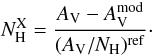${\mathit{N}}_{\mathrm{H}}^{\mathrm{X}}\mathrm{=}\frac{{\mathit{A}}_{\mathrm{V}}\mathrm{-}{\mathit{A}}_{\mathrm{V}}^{\mathrm{mod}}}{\mathrm{(}{\mathit{A}}_{\mathrm{V}}\mathit{/}{\mathit{N}}_{\mathrm{H}}{\mathrm{)}}^{\mathrm{ref}}}\mathrm{·}$(5)The total mass of hydrogen within the DG component (${\mathit{M}}_{\mathrm{H}}^{\mathrm{X}}$), the atomic (${\mathit{M}}_{\mathrm{H}}^{\mathrm{HI}}$), and CO-traced molecular gas (${\mathit{M}}_{\mathrm{H}}^{\mathrm{CO}}$), is estimated in the same way as in Planck Collaboration (2011a)${\mathit{M}}_{\mathrm{H}}^{\mathrm{X}\mathit{,}\mathrm{HI}\mathit{,}\mathrm{CO}}\mathrm{=}{\mathit{m}}_{\mathrm{H}}{\mathit{D}}^{\mathrm{2}}{\mathrm{\Omega }}_{\mathrm{pix}}\begin{array}{}\sum \end{array}{\mathit{N}}_{\mathrm{H}}^{\mathrm{X}\mathit{,}\mathrm{HI}\mathit{,}\mathrm{CO}}\mathit{,}$(6)where D is the distance to the gas, m_H the hydrogen atom mass, and Ω_pix the pixel solid angle. As in Planck Collaboration (2011a), we assumed the same distance to all gas components. We obtained ${\mathit{M}}_{\mathrm{H}}^{\mathrm{X}}\mathit{/}{\mathit{M}}_{\mathrm{H}}^{\mathrm{HI}}\mathrm{=}\mathrm{0.19}\mathrm{\pm }\mathrm{0.25}$ and ${\mathit{M}}_{\mathrm{H}}^{\mathrm{X}}\mathit{/}{\mathit{M}}_{\mathrm{H}}^{\mathrm{CO}}\mathrm{=}\mathrm{1.64}\mathrm{\pm }\mathrm{2.20}$. These values are expected to be both overestimated and underestimated, respectively, since the scale-height of the HI component is larger than that of the molecular one, with a probable intermediate scale-height for the DG component. The formal uncertainty in the DG mass is large and essentially results from the assumed uncertainty in ΔA_V/A_V and from our assumption that this uncertainty is an absolute error and therefore does not scale down with the number of independent measurements. This leads to a large uncertainty in the DG mass when most pixels in a region have low A_V values, but it is likely that our assumption about the nature of the errors overestimates the uncertainty.

Our DG mass is lower than found in Planck Collaboration (2011a), who deduced ${\mathit{M}}_{\mathrm{H}}^{\mathrm{X}}\mathit{/}{\mathit{M}}_{\mathrm{H}}^{\mathrm{HI}}\mathrm{\simeq }\mathrm{0.28}\mathrm{\pm }\mathrm{0.03}$ and ${\mathit{M}}_{\mathrm{H}}^{\mathrm{X}}\mathit{/}{\mathit{M}}_{\mathrm{H}}^{\mathrm{CO}}\mathrm{\simeq }\mathrm{1.18}\mathrm{\pm }\mathrm{0.01}$, but consistent with it, taking our large uncertainties into account. With the use of their X_CO value, we would obtain ${\mathit{M}}_{\mathrm{H}}^{\mathrm{X}}\mathit{/}{\mathit{M}}_{\mathrm{H}}^{\mathrm{CO}}\mathrm{\simeq }\mathrm{0.73}$. Our results lead to a DG mass equal to 17% of the total observed mass, close to the value of 22% derived by Planck Collaboration (2011a). Our study using extinction data therefore reveals slightly less DG mass than the same analysis based on FIR data. The difference between the two analyses is however insignificant owing to large uncertainties for this region of the sky.

3.1.2. Inner/outer Galaxy

We carried out the same analysis for the inner ( | l |  < 70°) and outer ( | l |  > 70°) Galaxy, at high Galactic latitudes ( | b |  > 10°). A difference appears in the (A_V/N_H)^ref ratio, with a higher value being found in the inner Galaxy ($\mathrm{(}\frac{{\mathit{A}}_{\mathrm{V}}}{{\mathit{N}}_{\mathrm{H}}}{\mathrm{)}}^{\mathrm{ref}}\mathrm{=}\mathrm{8.72}\mathrm{\times }{\mathrm{10}}^{-22}$ mag cm^-2) than the outer Galaxy ($\mathrm{(}\frac{{\mathit{A}}_{\mathrm{V}}}{{\mathit{N}}_{\mathrm{H}}}{\mathrm{)}}^{\mathrm{ref}}\mathrm{=}\mathrm{5.46}\mathrm{\times }{\mathrm{10}}^{-22}$ mag cm^-2). This result could illustrate the true large-scale variations in the dust abundance and reflect the large-scale metallicity gradient in our Galaxy.

From Fig. 2, one can see that the excess is more prominent in the inner Galaxy than the outer Galaxy. In addition, we note that the outer Galaxy appears to be more noisy at low gas column densities. This is likely because the outer Galaxy hosts fewer stars than the inner Galaxy, inducing larger uncertainties in the resulting extinction map. The reconciliation between the data and the linear fit, corresponding to the H₂-to-CO transition in the case of molecular DG, seems to occur at N_H ≃ 3 − 3.5 × 10²¹ cm^-2 (A_V ≃ 1.5–1.75 mag) in both the inner and the outer Galaxy.

In term of the DG mass, each part of the Galaxy has a different behavior. The inner regions contain a more enhanced DG component, with ratios ${\mathit{M}}_{\mathrm{H}}^{\mathrm{X}}\mathit{/}{\mathit{M}}_{\mathrm{H}}^{\mathrm{HI}}$ and ${\mathit{M}}_{\mathrm{H}}^{\mathrm{X}}\mathit{/}{\mathit{M}}_{\mathrm{H}}^{\mathrm{CO}}$ of about 0.24 and 2.43, respectively. In contrast, the DG mass in the outer Galaxy represents only 11% of the gas in the atomic phase and 74% of that in the CO-traced phase. This result indicates that the additional gas phase is essentially concentrated in the inner Galaxy. In a similar way, the X_CO factor appears to be larger in the inner Galaxy (X_CO = 2.28 × 10²⁰ H₂   cm^-2/(K   km   s^-1)) than its outer parts (X_CO = 1.67 × 10²⁰ H₂   cm^-2/(K   km   s^-1)).

3.1.3. Individual regions

Performing the analysis on individual regions requires the availability of enough pixels with and without DG, taking into account the limited extent of the CO survey. We were able to explore the A_V-N_H correlation in the following four regions:

• Taurus (200° < l < 160°;  −35° < b <  −10°);

• Orion (240° < l < 200°;  −30° < b <  −10°);

• Cepheus-Polaris (135° < l < 90°; 10° < b < 40°);

• Aquila-Ophiuchus (|l|  < 20°; 10° < b < 48°).

The results of the correlations for individual regions are presented in Fig. 3. Each environment has different dust properties, with ${{}^{\mathrm{\right(}}\frac{{\mathit{A}}_{\mathrm{V}}}{{\mathit{N}}_{\mathrm{H}}}^{\mathrm{\left)}}}^{\mathrm{ref}}$ ranging between 3.41 × 10^-22 and 6.99 × 10^-22 mag cm². Moreover, these regions are of great interest because they have distinctive gas properties. The X_CO factor in Orion and Aquila-Ophiuchus are larger than in the other regions. In addition, the former regions have a substantially large DG mass ratio relative to the atomic hydrogen, with ratios of 0.45 and 0.59, respectively. These large amounts of DG in Orion and Aquila-Ophiuchus are visible in Fig. 3 as a clear, large excess in the A_V-N_H plot. We checked that the excess was not due to contamination by YSOs. The color excess maps may indeed overestimate the true A_V if there is significant contamination by YSOs. In these two regions, we therefore also performed the correlation between extinction maps in the J band (A_J) and the gas tracers, because YSOs would induce an underestimation in the extinction maps (as opposed to the color excess maps). These results indicate that the large amount of DG is not caused by the presence of YSOs. Grenier et al. (2005) obtained a ratio ${\mathit{M}}_{\mathrm{H}}^{\mathrm{X}}\mathit{/}{\mathit{M}}_{\mathrm{H}}^{\mathrm{HI}}$ that is even larger than our results, in the Aquila-Ophiuchus-Libra region, with a ratio of 1. In contrast, they derived a value of 0.14 in Orion. They found a ratio of 0.33 for the Taurus-Perseus-Triangulum region, close to our value of 0.42 in the Taurus region. We note however that the individual regions defined in Grenier et al. (2005) are not exactly the same as the ones used in this paper. The A_V-N_H plot for Cepheus-Polaris does not display any noticeable excess. When comparing the DG mass with the CO one in the different clouds, we observe significant variations. We note values ranging from 0.17 in the Cepheus-Polaris region to 1.65 in Aquila-Ophiuchus, with values of 0.66 and 0.76 in Orion and Taurus. These ratios are however highly dependent on the value of the X_CO factor. The low uncertainty in the dark mass of the Taurus region is caused by the relatively large A_V values. The absolute uncertainty ΔA_V/A_V is larger in Cepheus-Polaris which corresponds to a large number of pixels at low A_V, inducing a considerable mass uncertainty.

The H₂-to-CO transition, which we determined by eye, appears at N_H ≃ 3.5 × 10²¹ cm^-2 (A_V ≃ 1.75 mag) in Taurus, N_H ≃ 6 × 10²¹ cm^-2 (A_V ≃ 3.0 mag) in Orion, N_H ≃ 3.5 × 10²¹ cm^-2 (A_V ≃ 1.75 mag) in Cepheus-Polaris, and N_H ≃ 4 × 10²¹ cm^-2 (A_V ≃ 2.0 mag) in Aquila-Ophiuchus. This transition seems to vary with environment. The position of the HI-to-H₂ transition is uncertain because of the noise in the extinction data at low gas-column densities. For this reason, we do not discuss its value further in this paper.

4. Discussion

The two quantities τ and A_V are in principle proportional. However, the estimate of the dust optical depth τ requires knowledge of the dust equilibrium temperature, requiring an additional step in the study of the dust/gas ratio, and additional assumptions that could bias the results. For instance, a single dust temperature is often assumed along the LOS. In addition, the temperature estimate depends on the assumption made about the emissivity spectral index β. In that sense, the use of extinction data is more straightforward. However, extinction data suffer from several defects, especially when producing the color excess map. Even if the X percentile method used to generate the map is a promising method, the resulting map can still be biased by missing extinction, inducing variations in the detection rate. The detection rate, i.e., the fraction of the detected A_V to the true total A_V integrated along the LOS, could vary as a function of both the Galactic coordinates and the distance to the clouds. To determine how much extinction we should miss in the adopted A_V map, we have carried out a test by applying the X percentile method to some artificial clouds set in the distribution of stars generated using the Besançon Model (Robin et al. 2003). We first prepared a spherical cloud having a Gaussian density distribution with a size of 6 pc (at FWHM) and a total extinction along the LOS of A_V = 10 mag at the center of the cloud. We then located the cloud at realistic coordinates and distances of some nearby clouds in the simulated star distribution, e.g., at (l,b) = (174.0°,  −13.5°) and at D = 150 pc for the Taurus cloud, and performed the X percentile method exactly in the same way as Dobashi (2011) did using the 2MASS PSC. Our results indicate that most of the individual clouds analyzed here are well-detected with a detection rate larger than 90% (i.e., the model cloud with A_V = 10 mag is detected as A_V > 9 mag), except for Orion whose detection rate is  ≃ 76%. General results show that nearby clouds (D < 500 pc), which represent most of the clouds at  | b |  > 10° in the A_V map, are clearly detected with a detection rate  > 80% for all directions. The low (A_V/N_H)^ref ratio derived in Orion could be the result of underestimating A_V in this region. Apart from this region, the (A_V/N_H)^ref ratios in Table 1 appear equal or larger than the reference value given by Bohlin et al. (1978), confirming that the X percentile method does not miss a substantial amount of extinction.

The determination of the X_CO conversion factor differs from one analysis to another. Our average value of 1.67 × 10²⁰ H₂   cm^-2/(K   km   s^-1) is close to the Galactic average (Strong & Mattox 1996) and the value derived by Dame et al. (2001) for  | b |  > 5°. A decrease in X_CO is observed from the inner to the outer high Galactic latitude sky. Most of the clouds observed in the Galactic extinction map at  | b |  > 10° are nearby local clouds, at a distance of about 200–500 pc, so we do not attribute the variations to the metallicity gradient (Rolleston et al. 2000), but instead to local variations. Arimoto et al. (1996), using CO data and virial masses, derived an average value near Sun of 2.8 × 10²⁰ H₂   cm^-2/(K   km   s^-1), with variations ranging from 2.09 × 10²⁰ to 3.74 × 10²⁰ H₂   cm^-2/(K   km   s^-1) with increasing Galactocentric radius. Abdo, et al. (2010) discovered a similar behavior, but with significant variations ranging from 0.87 × 10²⁰ H₂   cm^-2/(K   km   s^-1) in the Gould Belt to 1.9 × 10²⁰ H₂   cm^-2/(K   km   s^-1) in the Perseus arm. Finally, the Planck Collaboration (2011a) estimated an average value of 2.54 × 10²⁰ H₂   cm^-2/(K   km   s^-1) in the solar neighborhood. We also note that some of the studies included the dark component in their derivation of X_CO.

In their model to estimate the DG mass, Wolfire et al. (2010) predicted an HI-to-H₂ transition located at A_V ≃ 0.2 mag, which agrees with our findings. This result is however slightly lower than the value derived using FIR data (A_V ≃ 0.4 mag) following Planck Collaboration (2011a). However, in the latter case the HI-to-H₂ transition was determined by χ² minimization, whereas in our study it was done by eye, which can induce large uncertainties.

Moreover, the model predictions suggest a constant fraction of the molecular mass in the dark component of about 0.3 for an average extinction A_V around 8 mag. In cases of decreasing extinction, they found an increase in the dark mass fraction. In the framework of their model, this would indicate that a larger fraction of molecular gas is located outside the CO region. This fraction (f_DG) is computed as ${\mathit{f}}_{\mathrm{DG}}\mathrm{=}\frac{{\mathit{M}}_{\mathrm{H}}^{\mathrm{X}}}{{\mathit{M}}_{\mathrm{H}}^{\mathrm{X}}\mathrm{+}{\mathit{M}}_{\mathrm{H}}^{\mathrm{CO}}}\mathrm{·}$(7)Values of f_DG for each region are provided in Table 1. Over the entire high Galactic latitude sky, we derived f_DG = 0.62, with a larger value in the inner Galaxy (f_DG = 0.71) with respect to the outer Galaxy (f_DG = 0.43). For comparison, using the same definition of this quantity, the Planck Collaboration (2011a) obtained a value of f_DG ≃ 0.55 for the solar neighborhood. The Taurus and Aquila-Ophiuchus regions have a DG fraction of 0.43 and 0.62, respectively. These values are in good agreement with the results obtained by Grenier et al. (2005, see Table 1) in equivalent regions, with fractions of 0.3 and 0.6, for the Taurus and Aquila-Ophiuchus-Libra regions. These authors derived f_DG as low as 0.1 for Cepheus-Cassiopeia-Polaris and Orion, whereas Abdo, et al. (2010) deduced a value of 0.30 for Cepheus. We obtained f_DG equal to 0.15 and 0.40 in Cepheus-Polaris and Orion.

All these studies illustrate the existence of variations in the DG mass fraction. In our study, we have excluded the Galactic plane, where the most massive and bright molecular clouds are located. At the 36′ angular resolution, most of the pixels considered in our analysis have extinctions lower than 10 mag. In this case, f_DG values larger than 0.3 are expected following Wolfire et al. (2010), and this is indeed what is observed here.

Dust in the form of aggregates is likely to be more emissive than isolated grains, but aggregation is not expected to substantially affect absorption properties in the visible (Kohler et al. 2011). The detection of significant departure from linearity between extinction data and gas column densities, especially in Orion or Aquila-Ophiuchus, which exhibit the largest excess in Fig. 3, indicates that dust emissivity changes induced by grain aggregation is an unlikely explanation of the observed excess. As a consequence, grain coagulation can only be responsible for a small amount of the observed excess, and may explain some of the differences in the studies based on FIR data (Planck Collaboration 2011a) and visible extinction data (this work). Moreover, our results agree with the model prediction of Wolfire et al. (2010), favoring the hypothesis of pure H₂ gas (without CO molecules), surrounding the CO regions.

5. Summary

Using a recently revised all-sky extinction map, we have examined the correlation between the extinction and gas column densities derived from HI and CO observations. Our results can be summarized as follows:

• We have measured an excess of extinction at intermediate columndensities, relative to a linear-fit between A_V and observable gas. Thisexcess is observed over the whole high Galactic latitude sky, witha predominant amount being found toward the inner regions ( | l |  < 70°),and in particular in Aquila-Ophiuchus. This result confirms therecent detection of DG in the Planck data and implies that theeffect in the FIR is not due to changes in the dust optical propertiescaused by dust aggregation.

• We have derived an average dust extinction to gas ratio of (A_V/N_H)^ref = 6.53 × 10^-22 mag cm^-2 in the solar neighborhood, for an average X_CO = 1.67 × 10²⁰ H₂ cm^-2/(K km s^-1). The inner/outer Galaxy exhibits a higher/lower (A_V/N_H)^ref ratio (8.72 × 10^-22/5.46 × 10^-22 mag cm^-2), associated with a higher/lower X_CO factor (2.28 × 10²⁰/1.67 × 10²⁰ H₂ cm^-2/(K km s^-1). A significantly larger value, more than twice the value derived in the solar neighborhood is observed in the Aquila-Ophiuchus region. In contrast, the lowest X_CO value is found in Cepheus-Polaris.

• The results of our analysis agree with the theoretical predictions of modeling of the dark H₂ gas obtained to help explain the observed departure from linear-fits in the correlations.

• The DG mass derived is 19% of the atomic mass and 164% of that in the CO-traced gas in the solar neighborhood. It can reach up to 59% of the atomic gas in the Aquila-Ophiuchus region. Our DG mass estimates are slightly lower than that derived from FIR Planck data, but the difference is insignificant.

• We have estimated the fraction of the molecular mass in the dark component (f_DG) and found an average value of 0.62 in the solar neighborhood, with variations going from 0.43 to 0.71 in the outer and inner Galaxy. We have derived f_DG = 0.15, 0.43, 0.40, and 0.62 in the Cepheus-Polaris, Taurus, Orion, and Aquila-Ophiuchus regions, respectively.

• The HI-to-H₂ and H₂-to-CO transitions appear for A_V ≃ 0.2 and A_V ≃ 1.5 mag in the solar neighborhood, with variations from regions to regions.

Acknowledgments

D.P. was supported by the Centre National d’Etudes Spatiales (CNES). Part of this work was financially supported by Grant-in-Aid for Scientific Research (Nos. 22700785 and 22340040) of Japan Society for the Promotion of Science (JSPS). The authors would like to thank T. M. Dame for making the unpublished CO data available to them to perform this work.

References

Appendix A: WCS to HEALPix ancillary data transformation

The data used in this paper were transformed from their native WCS (world coordinate system) local projection into the HEALPix (Hierarchical Equal Area isoLatitude Pixelization) all-sky pixelization using the method described here in this Appendix. This method has also been used to produce HEALPix maps of a larger set of ancillary data, particularly in the context of the analysis of the Planck data². We note that the CO map used in this paper is not yet freely available, since the corresponding data have not been made public.

The HEALPix format allows us to store ancillary data on a single grid scheme on the sphere. This is advantageous since different data can then be compared on a pixel by pixel basis, without the need to project the data to a common grid. Ancillary data are available in the WCS convention and are usually stored as Flexible Image Transport System (FITS) files. In the following, we refer to the ancillary data as FITS maps. It is usually impractical to return to the raw ancillary data and directly reprocess the maps into the HEALPix pixelization. It is therefore necessary to project the FITS format data onto the HEALPix pixels. As the FITS and HEALPix pixels do not match each other in position, size, and shape, this requires some kind of interpolation, which must be done with the minimal loss of information and without altering the photometry of the original ancillary data. Here, we use a mosaicking method where we compute explicitly the surface of the pixel intersections, and use these values as weights to construct the HEALPix map.

The HEALPix pixels projected onto a local FITS map are shown in Fig. A.1. The calculations are performed for a HEALPix pixel size (given by the N_side HEALPix parameter) so that the corresponding HEALPix pixel size matches the Shannon criterion for the angular resolution of the data considered. This ensures that no spatial information is lost in the conversion and that the corresponding HEALPix and the FITS pixels have similar sizes. For a given FITS projection (i.e. from the astrometry information contained in the FITS header), we first identify the HEALPix pixels that intercept the sky area covered by the FITS map. For each of those HEALPix pixels, we identify the FITS pixels with a non-zero intersection. We then compute the surface fraction of the FITS pixels intersecting the HEALPix pixel ${\mathit{S}}_{\mathit{ih}}^{\mathit{if}}$, where “if” denotes the FITS pixel number and “ih” denotes the HEALPix pixel number.

The calculation is performed in the pixel space of the FITS map shown in Fig. A.1. We first compute the sky coordinates of the four corners of the considered HEALPix pixel. We then transform these coordinates into 2D pixel numbers (i, j) of the FITS image using standard routines and the astrometry information contained in the FITS header of the considered image. We then assume that the frontier of the HEALPix pixel is a straight line in the FITS image pixel frame. Although this is not exactly true, this is a very small approximation when the size of the HEALPix pixel is smaller or on the order of the FITS pixel size, which is always the case here. We then compute the surface of the corresponding intersection polygon, which has been normalized to that of the HEALPix pixel surface ${\mathit{S}}_{\mathit{ih}}^{\mathit{if}}$³.

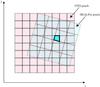Fig. A.1 Geometry of the HEALPix and FITS pixels.

The intersection geometry informations (if and ${\mathit{S}}_{\mathit{ih}}^{\mathit{if}}$) are stored in a table containing one entry per HEALPix pixel that has non-zero intersection with the considered FITS map. Calculations are carried and stored separately for each FITS map. We note that the above table can be easily inverted to a table with one entry per FITS pixel, giving the HEALPix pixel numbers intercepting it (ih) and the corresponding surface

fraction ${\mathit{S}}_{\mathit{if}}^{\mathit{ih}}$, which in turn can be used to perform reverse calculations projecting HEALPix maps onto local WCS projection.

The above intersection fractions are then used to compute HEALPix ancillary data value d_ih, given the FITS data d_if as 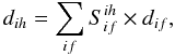${\mathit{d}}_{\mathit{ih}}\mathrm{=}\sum _{\mathit{if}}{\mathit{S}}_{\mathit{if}}^{\mathit{ih}}\mathrm{\times }{\mathit{d}}_{\mathit{if}}\mathit{,}$(A.1)where the summation is carried over all FITS pixels intersecting a HEALPix pixel ih.

When the data is composed of a collection of individual FITS maps, the calculation are performed for each map separately, while maintaining a map of the total weight, which allows us to evaluate average values in sky regions where individual maps overlap. We note that virtually all WCS projection types can be used, including the sixcube projection used for the COBE and FIRAS data.

All Tables

All Figures

	Fig. 1 Extinction map (AV) in mag. Regions in light blue are not covered by the combination of the Dame et al. (2001) and NANTEN CO surveys, and are not used in our analyses. The red boxes correspond to individual regions defined in Sect. 3.1.3.
In the text

Fig. 2 Correlation plots between extinction data (AV) and the total gas-column density (${\mathit{N}}_{\mathrm{H}}\mathrm{=}{\mathit{N}}_{\mathrm{H}}^{\mathrm{HI}}\mathrm{+}\mathrm{2}{\mathit{X}}_{\mathrm{CO}}{\mathit{W}}_{\mathrm{CO}}$) excluding the Galactic plane ( | b |  > 10°): high latitude sky (top panels), inner Galaxy (middle panels) and outer Galaxy (bottom panels). Left, middle, and right panels correspond respectively, to regions where no DG is detected (“no DG”) according to Planck Collaboration (2011a), where strong DG is detected (“DG”), and the entire region (“All”) (see Sect. 3.1). The color scale represents the density of pixels on a log scale. The yellow dots show the correlation binned in NH. The red lines show the best-fit linear correlation, constrained for the whole data in the “no DG” region. The short-dashed and long-dashed lines indicate the position of a departure from a linear fit, and the position where the correlation recovers a linear behavior, respectively.

In the text

Fig. 3 Correlation plots between extinction data (AV) and the total gas column density (${\mathit{N}}_{\mathrm{H}}\mathrm{=}{\mathit{N}}_{\mathrm{H}}^{\mathrm{HI}}\mathrm{+}\mathrm{2}{\mathit{X}}_{\mathrm{CO}}{\mathit{W}}_{\mathrm{CO}}$) in various regions excluding the Galactic plane ( | b |  > 10°), from top to bottom the Cepheus-Polaris, Taurus, Orion, and Aquila-Ophiuchus regions. Left, middle, and right panels correspond respectively, to regions where no DG is detected (“no DG”) according to Planck Collaboration (2011a), where strong DG is detected (“DG”), and the entire region (“All”) (see Sect. 3.1). The color scale represents the density of pixels on a log scale. The description of the yellow dots, red, and dashed lines is given in the caption of Fig. 2.

In the text

	Fig. A.1 Geometry of the HEALPix and FITS pixels.
In the text

References

- Abdo, A. A., Ackermann, M., Ajello, M., et al. 2010, ApJ, 710, 133 [NASA ADS] [CrossRef] [Google Scholar]
- Arnal, E. M., Bajaja, E., Larrarte, J. J., et al. 2000, A&AS, 142, 35 [NASA ADS] [CrossRef] [EDP Sciences] [Google Scholar]
- Arimoto, N., Sofue, Y., & Tsujimoto, T. 1996, PASJ, 48, 275 [NASA ADS] [CrossRef] [Google Scholar]
- Bajaja, E., Arnal, E. M., Larrarte, E., et al. 2005, A&A, 440, 767 [NASA ADS] [CrossRef] [EDP Sciences] [Google Scholar]
- Bernard, J.-P., Reach, W., Paradis, D., et al. 2008, AJ, 136, 919 [NASA ADS] [CrossRef] [Google Scholar]
- Bohlin, R. C., Savage, B. D., & Drake, F. J. 1978, ApJ, 224, 132 [NASA ADS] [CrossRef] [Google Scholar]
- Cambrésy, L. 1999, A&A, 345, 965 [NASA ADS] [Google Scholar]
- Cardelli, J. A., Clayton, G. C., & Mathis, J. S. 1989, ApJ, 345, 245 [NASA ADS] [CrossRef] [Google Scholar]
- Dame, T. M. 2011 [arXiv:1101.1499] [Google Scholar]
- Dame, T. M., Hartmann, D., & Thaddeus, P. 2001, ApJ, 547, 792 [NASA ADS] [CrossRef] [Google Scholar]
- Dobashi, K. 2011, PASJ, 63, S1 [NASA ADS] [CrossRef] [Google Scholar]
- Dobashi, K., Bernard, J.-P., Hughes, A., et al. 2008, A&A, 484, 205 [NASA ADS] [CrossRef] [EDP Sciences] [Google Scholar]
- Dobashi, K., Bernard, J.-P., Kawamura, A., et al. 2009, AJ, 137, 5099 [NASA ADS] [CrossRef] [Google Scholar]
- Dobashi, K., Marshall, D. J., Shimoikura, T., & Bernard, J.-P. 2012, PASJ, submitted [Google Scholar]
- Fukui, Y., Onishi, T., Abe, R., et al. 1999, PASJ, 51, 571 [Google Scholar]
- Grenier, I. A., Casandjian, J. M., & Terrier, R. 2005, Science, 307, 1292 [NASA ADS] [CrossRef] [PubMed] [Google Scholar]
- Hartmann, D., & Burton, W. B. 1997, Atlas of Galactic Neutral Hydrogen (Cambridge, UK: Cambridge University Press) [Google Scholar]
- Kohler, M., Guillet, V., & Jones, A. 2011, A&A, 528, A96 [NASA ADS] [CrossRef] [EDP Sciences] [Google Scholar]
- Langer, W. D., Velusamy, T., Pineda, J. L., et al. 2010, A&A, 521, A17 [NASA ADS] [CrossRef] [EDP Sciences] [Google Scholar]
- Lada, C. J., Lada, E. A., Clemens, D. P., & Bally, J. 1994, ApJ, 429, 694 [NASA ADS] [CrossRef] [Google Scholar]
- Leroy, A., Bolatto, A., Stanimirovic, S., et al. 2007, ApJ, 658, 1027 [NASA ADS] [CrossRef] [Google Scholar]
- Meyerdierks, H., & Heithausen, A. 1996, A&A, 313, 929 [NASA ADS] [Google Scholar]
- Planck Collaboration 2011a, A&A, 536, A17 [NASA ADS] [CrossRef] [EDP Sciences] [Google Scholar]
- Planck Collaboration 2011b, A&A, 536, A24 [Google Scholar]
- Reach, W. T., Koo, B., & Heiles, C. 1994, ApJ, 429, 672 [NASA ADS] [CrossRef] [Google Scholar]
- Robin, A. C., Reylé, C., Derrière, S., & Picaud, S. 2003, A&A, 409, 523 [NASA ADS] [CrossRef] [EDP Sciences] [Google Scholar]
- Rolleston, W. R. J., Smartt, S. J., Dufton, P. K., & Ryans, R. S. I. 2000, A&A, 363, 537 [NASA ADS] [Google Scholar]
- Roman-Duval, J., Israel, F. P., Bolatto, A., et al. 2010, A&A, 518, A74 [Google Scholar]
- Rowles, J., & Froebrich, D. 2009, MNRAS, 395, 1640 [NASA ADS] [CrossRef] [Google Scholar]
- Skrutskie, M. F., Cutri, R. M., Stiening, R., et al. 2006, AJ, 131, 1163 [NASA ADS] [CrossRef] [Google Scholar]
- Spitzer, L. 1978, Physical Processes in the Interstellar Medium (New-York: Wiley-Interscience) [Google Scholar]
- Strong, A. W., & Mattox, J. R., A&A, 308, 21 [Google Scholar]
- Wolfire, M. G., Hollenbach, D., & McKee, C. F. 2010, ApJ, 716, 1191 [NASA ADS] [CrossRef] [Google Scholar]