| Issue |
A&A
Volume 543, July 2012
|
|
|---|---|---|
| Article Number | A57 | |
| Number of page(s) | 15 | |
| Section | Extragalactic astronomy | |
| DOI | https://doi.org/10.1051/0004-6361/201118200 | |
| Published online | 27 June 2012 | |
Compact radio emission from z ~ 0.2 X-ray bright AGN⋆
1 I. Physikalisches Institut, Universität zu Köln, Zülpicher Str. 77, 50937 Köln, Germany
e-mail: This email address is being protected from spambots. You need JavaScript enabled to view it.
2 Max-Planck-Institut für Radioastronomie, Auf dem Hügel 69, 53121 Bonn, Germany
Received: 4 October 2011
Accepted: 13 April 2012
Abstract
Context. The radio and X-ray emission of active galctic nuclei (AGN) appears to be correlated. The details of the underlying physical processes, however, are still not fully understood, i.e., to what extent the X-ray and radio emission is originating from the same relativistic particles, or from the accretion-disk, or corona, or both.
Aims. We study the cm radio emission of an SDSS/ROSAT/FIRST matched sample of 13 X-raying AGN in the redshift range 0.11 ≤ z ≤ 0.37 at high angular resolution with the goal of searching for jet structures or diffuse, extended emission on sub-kpc scales.
Methods. We used MERLIN at 18 cm for all objects and Western EVN at 18 cm for four objects to study the radio emission on scales of ~500 pc and ~40 pc for the MERLIN and EVN observations, respectively.
Results. The detected emission is dominated by compact nuclear radio structures. We find no kpc collimated jet structures. The EVN data indicate compact nuclei on 40 pc scales, with brightness temperatures typical for accretion-disk scenarios. Comparison with FIRST data shows that the 18 cm emission is resolved out up to 50% by MERLIN. Star-formation rates based on large aperture SDSS spectra are generally too low to produce considerable contamination of the nuclear radio emission. We can, therefore, assume the 18 cm flux densities to be produced in the nuclei of the AGN. Together with the ROSAT soft X-ray luminosities and black-hole mass estimates from the literature, our sample objects closely follow the Merloni et al. fundamental plane relation, which appears to trace the accretion processes. Detailed X-ray spectral modeling from deeper hard X-ray observations and higher angular resolution at radio wavelengths are required to make more progress in separating jet and accretion related processes.
Key words: galaxies: nuclei / radio continuum: galaxies / techniques: interferometric
Appendix A is available in electronic form at http://www.aanda.org
© ESO, 2012
1. Introduction
X-rays have turned out to be efficient tracers of nuclear activity in active galactic nuclei (AGN, Brandt & Hasinger 2005). Current models suggest that the observed X-rays are produced in the accretion flow onto the central supermassive black hole (SMBH), with soft X-rays typically originating from the accretion disk and hard, comptonized X-rays from a corona surrounding the accretion disk (e.g., Shields 1978; Haardt & Maraschi 1991; Perola et al. 2002).
Related to the accretion phenomenon is the observation of jets, outflows that consist of charged particles (primarily electrons) accelerated to relativistic velocities. The electrons give rise to the observed synchrotron spectrum at radio frequencies (e.g., Bridle & Perley 1984). Some AGN, however, show flat radio spectra, which are interpreted as self-absorbed synchrotron radiation of multiple jet knots (e.g., Cotton et al. 1980).
Several studies of radio and X-ray detected AGN have resulted in an apparent correlation between the radio and X-ray luminosities (e.g., Salvato et al. 2004; Brinkmann et al. 2000), suggesting a common physical origin of both phenomena. Together with the associated black-hole mass, these two values determine the location of objects in the fundamental plane (FP) of black-hole activity (e.g., Falcke et al. 2004; Merloni et al. 2003). The physical relation between the three properties is still unclear, however. Several structural components (accretion disk, corona, jet, disk wind) and physical processes (synchrotron, (inverse) Compton, bremsstrahlung, relativistic beaming) can contribute to the total radio and X-ray output (e.g., Narayan et al. 1998; Heinz & Merloni 2004; Yuan et al. 2005; Steenbrugge et al. 2011). Their relative importance appears to depend on the accretion efficiency, the black-hole mass, and potentially the black-hole spin (e.g., Körding et al. 2006; Sikora et al. 2007). This, however, renders a simple interpretation of the FP impractical, i.e. identification of physical processes by locus in the FP, at least for individual objects. Indeed, there appears to be a range of different FPs, depending on object class, i.e. the predominant physical processes. Detailed analyses are, therefore, necessary, to properly separate star formation, accretion flow, and jet emission from each other in the circumnuclear environment of AGN. This is especially important at higher redshifts, for which the probed linear scales become increasingly larger and the surface brightnesses increasingly dimmer. Sensitive, high angular resolution observations at radio wavelengths are helpful in this respect, because they allow one to assess the presence and influence of jet emission, relativistic beaming, and star formation based on radio morphology and radio spectral index. For example, Japanese VLBI Network (JVN) milli arc-second angular resolution (~4 mas) observations of three z ~ 0.2 RL NLS1 galaxies (Doi et al. 2007) show unresolved nuclei on pc scales and brightness temperatures as well as spectral properties indicative for relativistically beamed emission. Ulvestad et al. (2005) carried out VLBA imaging of RQ QSOs at mas resolution. Two objects of their sample are at z ≈ 0.2 and either show a jet or a self-absorbed, compact synchrotron source. According to the ratio of their X-ray and radio fluxes, they appear to be rather radio-loud (cf., Terashima & Wilson 2003). Based on VLBA observations, Blundell & Beasley (1998) found strong evidence for jet-producing central engines for some of their RQ QSOs in the form of relativistically beamed radio emission. Leipski et al. (2006) presented VLA configuration A and B imaging of z ≈ 0.2 RQ QSOs and low-z Seyfert galaxies. The radio structures found in these QSOs resemble those of jets and outflows, and the authors proposed that RQ QSOs are up-scaled versions of Seyfert galaxies. The question remains, however, why these objects cannot form the powerful jets that have been found in RL QSOs, although they possess the jet-producing central engine. Steenbrugge et al. (2011) followed the idea that the radio emission of RQ QSOs is produced by free-free emission in the optically thin part of an accretion disk wind. Studying RQ Palomar Green QSOs (PG QSOs) in X-rays and in the radio at sub arc-second resolution, Steenbrugge et al. found that only in two out of twenty objects, bremsstrahlung might contribute to the nuclear radio emission. The QSOs investigated in the literature so far are among the brightest members of the intermediate-redshift AGN population. Studying the radio properties of less luminous QSOs, therefore, allows one to probe and extend the parameter space of relevant physical processes to less powerful and more abundant QSOs.
In the following, we present radio interferometric 18 cm continuum observations of 13 optically selected, X-ray bright AGN to investigate the radio/X-ray correlation for intermediate redshift AGN in more detail. Section 2 describes the sample and Sect. 3 the observations. Section 4 presents the results and a discussion in the context of the radio/X-ray correlation, concluded by a summary in Sect. 5. The appendix provides notes on individual targets. Throughout this work, we use a cosmology with H0 = 70 km s-1 Mpc-1, Ωm = 0.3, and ΩΛ = 0.7 (Spergel et al. 2003).
2. The sample
The space density of luminous AGN is very low in the nearby Universe (e.g., Schulze et al. 2009). To study the (circum-) nuclear energetics in these AGN, one has to resort to a larger cosmological volume. Increased projected linear scales and surface-brightness dimming, however, make more distant galaxies harder to interpret. A proper separation of Seyfert and star-formation features benefits from radio-interferometric observations. These are possible with current observatories like the Multi-Element Radio Linked Interferometer Network (MERLIN) or the European Very Long Baseline Interferometer Network (EVN). Observations of luminous, intermediate-redshift AGN have the potential to impart means to connect the physical drivers in terms of fueling and feedback of low-redshift and less powerful AGN to those of high-redshift, very powerful AGN.
The 13 targets1 presented in this work are based on a cross-match between the Sloan Digital Sky Survey Second data release (SDSS DR2, Abazajian et al. 2004) and the ROSAT All Sky Survey (RASS, Voges et al. 1999). From the SDSS, we have chosen only those objects for which an optical spectrum has been measured. The SDSS/RASS pairs were subsequently matched with the VLA Faint Images of the Radio Sky at Twenty centimeters survey (FIRST, Becker et al. 1995). FIRST provides better than 5′′ angular resolution. SDSS, RASS, and FIRST are very well matched in terms of sky coverage and sensitivity (Anderson et al. 2003). For this pilot study, we specifically selected intermediate-redshift objects (0.1 < z < 0.4) from the matched sample that lie close to the classical Seyfert/QSO luminosity demarcation (i.e., Mi = −22 Schneider et al. 2003) and that encompass different spectral types of AGN (i.e., Seyfert 1, Narrow Line Seyfert 1, LINER, radio galaxy; cf., Table 1 for individual classes). These targets are less luminous for a given redshift than the well-studied PG QSOs (by about 2 mag at V band; cf., Laor & Behar 2008). Furthermore, we selected only FIRST-unresolved RQ to radio-intermediate objects. They have milli-Jansky flux densities, making them accessible for sensitive radio interferometric observations and allow us to investigate the nature of their core radio emission. The details of the X-ray/optical matching are described in Zuther et al. (2009). The matched sample, at this point, is by no means complete, because we selected specific AGN classes from the quite small initial crossmatched sample (about 100 objects). Resorting to more recent versions of crossmatched samples (e.g., Anderson et al. 2007; Vitale et al. 2012; Zuther et al., in prep.; based on more recent SDSS data releases), allows selecting statistically more relevant subsamples of individual AGN classes (e.g., NLS1s) for high angular resolution follow-up studies.
Basic SDSS, ROSAT, and FIRST characteristics of the sample.
Table 1 lists basic source parameters: ID2 (1), SDSS name (2), redshift (3), spectroscopic class (4), local environment (5), extinction-corrected SDSS absolute i-band psf magnitude (6), FIRST 20 cm peak flux density in mJy (7), FIRST beam size in sqarcsec (8), logarithm of radio loudness (9), logarithmic units of ROSAT 0.1 − 2.4 keV flux in erg s-1 (10), and logarithmic units of the black-hole mass in M⊙ (11). The absolute i-band magnitude was calculated assuming a power-law3 at visible wavelength with index αvis = 0.5 (e.g., Anderson et al. 2003) and a K-correction of the form Fi = Fo(1 + z)α − 1 (Peterson 1997). The radio loudness is defined as R∗ = f5 GHz/f2500 Å (e.g., Kellermann et al. 1989). In the radio domain we used a power-law index αr = 0.7 (e.g., Hill et al. 2001) to estimate the rest-frame 6 cm flux density. The 2500 Å flux density was estimated from the SDSS gPSF magnitude, using the above αvis. Objects clearly above log R∗ > 1 are usually described as radio-loud (RL). Very powerful ones can even reach R∗ > 3 (cf., Ivezić et al. 2002). X-ray fluxes were computed by converting the X-ray counts to flux using PIMMS4 and assuming an absorbed power-law with an energy index αX = 1.5 (cf., Anderson et al. 2003)5. The absorbing column densities are Galactic values and were determined from the H I map of Dickey & Lockman (1990). Black-hole masses were taken from the literature (see Table 1) and are based on a combination of the measurements of the width of broad components of hydrogen recombination lines and the luminosity-radius relation of broad-line AGN (e.g., Kaspi et al. 2005). For (SDSS J150407.51-024816.5 [4] and SDSS J010649.39+010322.4 [5]), we measured the [SII] line dispersions as tracers of the bulge stellar velocity dispersion from their SDSS spectra and employed the M• − σ∗ relation as discussed in Komossa & Xu (2007). However, the values are only intended to give a rough idea of the involved black-hole masses. SDSS J162332.27+284128.7 [9] is a BL Lac, SDSS J092710.60+532731.6 [12] is a passive galaxy, and both sources show no spectral feature that can be used for SMBH mass-estimates.
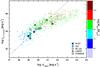 |
Fig. 1 0.1−2.4 keV X-ray vs. 20 cm FIRST peak luminosity. Symbols of our sources are indicated in the legend and correspond to spectroscopic types. Colors are coded according to the black-hole mass. Open symbols are for objects without available black-hole mass. For comparison, we present SDSS/FIRST/ROSAT-based broad-line AGN (BLAGN) from Li et al. (2008, × correspond to RQ and +. The dashed line is the linear correlation for RQ QSO of Brinkmann et al. (2000). |
Figure 1 shows the radio/X-ray correlation for our sample. For comparison we also show the SDSS/ROSAT/FIRST-based broad line AGN (BLAGN) sample of Li et al. (2008), together with the fit for RQ QSOs from (Brinkmann et al. 2000). The BLAGN sample is split into an RQ ( × ) and an RL ( + ) subsample. The radio-loud objects harbor more massive black holes than the RQ objects, though the dependence on black-hole mass appears to be most intense at lower radio powers (cf., Fig. 4 in Li et al. 2008). The RQ correlation has a slope of unity, indicating that the core radio emission is a direct tracer of the nuclear activity. Our targets follow the RQ relation closely, with the exception of target 11, which has a strong, extended jet component. At high radio powers, the RL BLAGN significantly deviate from the RQ relation, indicating that the jet component becomes dominant. If the X-ray emission still originates from (or close to) the accretion disk, while the radio emission is coming from the jet, then a deviation from the RQ correlation is expected.
3. MERLIN and EVN observations
We acquired 18 cm continuum snapshots of the 13 X-ray bright AGN introduced in Sect. 2 using MERLIN. For four objects we also obtained 18 cm Western EVN (using the stations Effelsberg, Medicina, Westerbork, Onsala [85 ft.], Torun, Noto, and Jodrell Bank [Lovell]) observations at higher angular resolution. Target 4 was furthermore studied with the same Western EVN at 6 cm. All observations were carried out in phase-referencing mode, i.e. the target scans were alternated with scans of a nearby phase reference. The observations were distributed over several hour angles to ensure a more homogeneous uv coverage. Table 2 gives an overview of the individual observing runs, including the date of observations (2), radio observatory (3), exposure time (4), and the associated phase calibrators (5). For the MERLIN data, we checked the suitability of the pipeline results (amplitude-, phase calibration, flagging of the phase calibrator) and applied additional flagging of the target amplitudes and phases before imaging with the data reduction package AIPS6 (Wells 1985). For the EVN data, we carried out flagging, amplitude/phase calibration and fringe-fitting with AIPS before imaging, according to standard reduction recipes7.
4. Results and discussion
Cleaning and self-calibrating the images with Difmap8 (Shepherd 1997), employing natural weighting, resulted in the Stokes-I maps9 presented in Figs. 2 and 3. The restoring beam sizes and orientation are indicated in the lower left corner of the maps. Typical beam sizes are 290 × 170 mas for MERLIN and 19 × 12 mas for EVN, corresponding to linear scales of about 950 × 560 pc and 63 × 40 pc, respectively. The contours represent multiples of the standard deviation, σ, of off-source regions in the final reconstructed images, as listed in Table 310. The table furthermore lists source properties such as peak flux density, major and minor axes of a Gaussian fit to the central component, and the extent of the central component, measured as  (cf., Ivezić et al. 2002). Sources with ϵ > 1 are extended.
Journal of 18 cm observations.
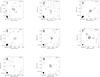 |
Fig. 2 Maps of the MERLIN 18 cm reconstructed images of the detected sources (detection threshold 3σ). Contours refer to − 2 (dashed), 2, 3, 4, 5, and 6 times the σ in the image. Except for sources 7 and 9, for which the contours refer to −2, 2, 3, 4, 8, 16, 32, ... times the σ. All σ values are given in Table 3. The beams are indicated in the bottom left corner of the maps. North is up, East is left. Sources with EVN follow-up observations are shown in Fig. 3. |
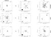 |
Fig. 3 The first two columns present MERLIN and EVN 18 cm reconstructed maps. The third column shows the MERLIN 18 cm map of source 4 in the first row. The second row shows the EVN 6 cm map including the eastern and western components. In the third row we present a close-up of the eastern component in the EVN 18 cm map. The western component was not detected. We present maps of the cleaned images of the detected sources (detection threshold 3σ). Contours refer to − 3 (dashed), 3, 4, 8, 16, ... times the σ in the images. The σ values are given in Table 3. The beams are indicated in the bottom left corner of the maps. North is up, East is left. |
All targets were detected with MERLIN and EVN, except SDSS J134420.87+663717.6 [13]. Noise levels range from 0.07 − 0.6 mJy in the MERLIN images and 0.06−1.14 mJy in the EVN images. As can be deduced from the maps, all detected sources are dominated by a nuclear component. The extent parameter indicates that these nuclear components are marginally resolved (ϵ ~ 1.16). Note that the boundary between unresolved and resolved source is not sharp, since errors in the estimation of peak and integrated flux densities have to be taken into account. Assuming 10% errors of the flux measurements (which is the mean error for all our measurements), results in a ~10% error for ϵ. This means that ϵ = 0.9 and ϵ = 1.1 have the same meaning. Targets SDSS J030639.57+000343.1 [7] and SDSS J080644.41+484149.2 [11] show the most extended structures according to their ϵ. A special case is target [4], for which we detected a second strong nuclear component (see also Appendix A for a more detailed discussion). This is the only source that was also targeted at 6 cm. Both components were detected at 6 cm, but only the stronger component was detected at 18 cm (Fig. 3). Bad weather conditions during the 18 cm run could have partially been responsible for a reduced sensitivity outside the image center.
Figure 4 displays the brightness temperature versus the radio-derived star-formation rate (SFR). As discussed below (Sect. 4.2), the SFR is proportional to the radio luminosity density. Therefore, the figure also displays the variation of peak flux density with the used array (VLA – MERLIN – EVN; i.e., the probed angular scales). For most sources, a trend of decreasing peak flux densities of the central marginally resolved point source with increasing angular resolution is evident. This is consistent with the idea of attributing part of the radio emission (up to 50% from FIRST to MERLIN) to extended jet structures or star formation. These features are just resolved out by the longer baselines. Variability of the nuclear source can also account to some degree for the differences between the multi-epoch/multi-aperture data. As will be discussed in the next section, the increased peak flux densities for some sources (1, 4, 10, 12) at later epochs clearly point toward variability. For sources whose peak flux density at later epochs is decreasing, we cannot clearly distinguish between the two effects.
4.1. Extended emission
The sources of this sample – except target 11, which shows a compact core plus two distant lobes – are unresolved on FIRST scales. We can, therefore, compare the integrated flux density in the MERLIN images, Fpeak × ϵ2, with that of the FIRST peak flux densities (Table 3)11. Four (5, 6, 8, 12) of the 11 MERLIN detections (ignoring the double source 4 for the moment) are clearly fainter on MERLIN than on FIRST scales, indicating resolved extended emission. The resolved fractions reach up to 70%. Another four sources (2, 3, 9, 10) have integrated MERLIN flux densities similar to the FIRST peak flux density, indicating that most of the flux is still contained in the compact nuclear component. The remaining three sources (1, 7, 11) are clearly brighter on MERLIN scales, indicating variability. In addition to source intrinsic processes, interstellar scintillation in our Galaxy can be responsible for part of the observed variability (e.g., Draine 2011). This is particularly important in the 3−8 GHz regime and caused by changing sight lines through the interstellar medium to the target during the motion of the Earth around the Sun. It has been observed that the variability amplitude of compact (on VLBI scales) cores of QSOs related to this phenomenon is typically up to 25% (e.g., Quirrenbach et al. 1992). We therefore checked the 60 μm and 100 μm IRAS maps around the positions of our sample objects for Galactic cirrus emission (cf., Jakobsen et al. 1987) and the maps for local (within a few parsecs) turbulent warm interstellar clouds (Linsky et al. 2008). We found that scintillation potentially contributes to the variability of our sources. In terms of differential cloud velocity (Linsky et al. 2008), sources 10 and 12 are the least and source 1 is most strongly affected by scintillation. Without any additional correction for this effect, the measured core fluxes of our targets are constant on that level, and excess variation is most likely due to source intrinsic properties (i.e., extended emission or variability of the central engine). Nevertheless, our basic conclusions regarding the radio loudness and the location in the fundamental plane, as discussed in the following sections, are not hampered by this effect. More (pseudo-simultaneous) multiwavelength observations are required to resolve the ambiguity between variability caused by jet/AGN or supernovae or interstellar scintillation contributions.
4.2. Importance of star formation
4.2.1. Brightness temperatures
The brightness temperature, TB, helps distinguishing between emission mechanisms. The angular size of the restoring beam can be used to determine TB, corresponding to the unresolved nuclear radio flux: 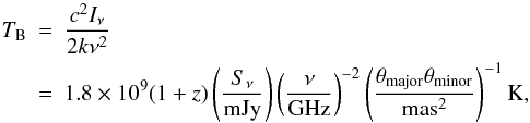 (1)where c is the speed of light, ν the frequency, k the Boltzmann constant, and Iν the specific monochromatic intensity, which is the specific flux density divided by the solid angle Ω, the extent of the radio emitter. The solid angle is approximately Ω ≈ θmajor × θminor of the unresolved source component. The factor (1 + z) accounts for the redshift of the source. The typical temperature of an HII region is on the order of 104 K. Brightness temperatures well above 104 K (typical for star-forming galaxies, e.g., Condon et al. 1982), are probably not caused by star formation (cf., discussion in Krips et al. 2007). The effective temperature of radiation for classical accretion disks is in the range 105 − 107 K (cf., Narayan et al. 1998). Brightness temperatures in excess of 107 K are related to nonthermal processes, at very high levels (>109 K) supposedly to relativistically beamed jet emission (e.g., Readhead 1994). Table 3 lists TB for the individual measurements (FIRST, MERLIN, EVN). The brightness temperatures for given angular sizes vary between 102 − 4 K for FIRST, 104 − 6 K for MERLIN, and 107 − 8 K for EVN; clearly increasing with increasing angular resolution. Brightness temperatures of the unresolved VLBA cores of RQQs are about 108 − 9 K (Ulvestad et al. 2005), while luminous quasars can exhibit brightness temperatures of up to 1012 K (e.g., Kellermann & Pauliny-Toth 1969). At least for the EVN data the values are too high to be dominated by star formation.
4.2.2. Star-formation indicators
A large body of work on star-forming galaxies shows correlations between X-ray/FIR (e.g., David et al. 1992), and radio/FIR (e.g., Condon et al. 1991), as well as calibrations of supernova and SFRs (e.g., Condon 1992; Hill et al. 2001; Hopkins et al. 2003; Bell 2003), which allows us to test the hypothesis that the nuclear emission is dominated by star formation.
First, we can estimate SFRs and FIR luminosities from our radio measurements. We used the 18 cm flux densities directly, since for reasonably flat spectra of radio emission the differences between 18 cm and 20 cm flux densities are negligible. Star-formation rate is, according to Bell (2003), related to the 20 cm luminosity density by  (2)The estimated SFRs for the FIRST, MERLIN, and EVN measurements are listed in Table 3. For about half of the sources the SFRs are > 100 and reach up to 104 M⊙ yr-1. Hopkins et al. (2003) find SFRs ≲ 100 M⊙ yr-1 for most of their SDSS-based sample of inactive galaxies. There are extreme examples of starbursts/interacting galaxies with SFRs of up to 1000 M⊙ yr-1 (cf., Kennicutt 1998). These objects, however, are ultraluminous infrared galaxies (ULIGs, e.g., Sanders & Mirabel 1996). We can also estimate the infrared (IR) flux if all radio emission is due to star formation, i.e. re-radiation of hot dust. We used the radio-SFR in Eq. (4) of Kennicutt (1998). For most of our objects the estimated IR luminosity falls in the regime of ULIGs. As such, they should have been detected by IRAS12.
MERLIN, EVN measurements, basic source parameters, and derived brightness temperatures, star-formation rates.
Supernovae are the end product of massive star formation. There appear to be exceptionally bright type-2 radio supernovae (RSNe). Following Hill et al. (2001), we compared our core flux densities with that of one of the brightest supernovae, SN1986J in NGC 891 (Weiler et al. 1990) shifted to the average redshift of our sample (z ~ 0.2). The 20 cm and 6 cm light curves peak at about 130 mJy. Our sample is about 1000 times more distant than NGC 891. To contribute significantly to the unresolved core emission, about 10 − 100 RSNe have to be involved. This is quite high, especially when considering the small volume sampled by the EVN observations (cf., Terlevich et al. 1992; Muxlow et al. 1994). Furthermore, assuming that the entire radio flux has a non-thermal origin, we can estimate the type-II supernova rate (SNR) according to Condon & Yin (1990):  (3)where α ~ − 0.8 is the nonthermal radio spectral index and LNT is the nonthermal component of the radio emission. Table 3 lists the estimated SNRs, which range from 0.1 − 83 yr-1. Starburst galaxies show SNRs on the order of ≲ 10 yr-1 (e.g., Mannucci et al. 2003), while Seyferts, with some exceptions, show SNRs on the order of ≲ 1 yr-1 (e.g., Hill et al. 2001; Laine et al. 2006).
Furthermore, we can use the the [OII]λ3728 Å luminosity, measured from the SDSS spectra, to estimate SFRs (e.g., Hopkins et al. 2003; Kennicutt 1998). It has been demonstrated that [OII] can also be used as a star-formation tracer in AGN (Ho 2005), and we will show that consistently, star formation is not significantly contaminating the nuclear emission. In high ionization type-1 AGN, flux ratios of [OII]/[OIII] typically range from 0.1 − 0.3 (Ho 2005, and references therein). Excess [OII] emission can then be attributed to star formation (cf., Villar-Martín et al. 2008). In our sample the median [OII]/[OIII] = 0.53, ranging from 0.13 to 4.9. Except for the two LINER galaxies [4, 5], which show the highest ratio in excess of a factor of about 15 over the typical type-1 AGN value, the ratios are quite similar to type-1 ionization. We followed the prescription of Ho (2005) in estimating [OII]-based SFRs. At this point we neglected excitation of [OII] via shocks. These might be important for LINERs (Heckman 1980) and in such cases, we overpredict the [OII]-based SFRs. With the Kennicutt (1998) calibration, we then found a median SFR of about 7.3 M⊙ yr-1, ranging from 0.4 to 71 M⊙ yr-1. This demonstrates that star formation contributes to the overall emission. However, inverting Eq. (2) to estimate radio luminosities based on the [OII]-derived SFRs and comparing with Table 3, especially with those SFRs derived from our MERLIN and EVN data, shows that star formation cannot explain the compact radio emission of our sources. The [OII]-based radio luminosities are at least an order of magnitude below those of the observed radio luminosities. There appear to be two exceptions, sources [5] and [6], for which [OII] and radio SFRs are on the same order of magnitude and are comparably small. Target [5] is one of the two LINER galaxies in our sample. The fact that the SFRs are of the same order of magnitude might be misleading, since part of the [OII] emission is likely to be excited by shocks, as mentioned above. Note that the 3′′ diameter SDSS fibers probe galactic scales on the order of 10 kpc at the average redshift of our sample, while MERLIN probes ten times smaller scales. In that sense, the SDSS fibers much better couple to the FIRST beam size of about 5′′ and probably much of the star formation is extended throughout the host galaxies. A direct comparison of the MERLIN and EVN based with the [OII] based SFRs has to be taken with caution and should only be regarded as a coarse indicator for the contribution of star formation to the radio emission.
Figure 4 summarizes the situation based on brightness temperature and radio SFR. With higher angular resolution (MERLIN) part of the emission is resolved out. The exceptions mentioned at the end of the previous paragraph consistently are on the left side of the diagram. With still increasing angular resolution (EVN), however, the nuclear emission is rather unresolved, the SFR remains constant, and the brightness temperature increases. The EVN cores are, therefore, likely due to nonstellar nuclear processes, which is consistent with the AGN nature of the visible spectra.
 |
Fig. 4 Brightness temperature vs. star-formation rate, both estimated from radio flux densities. The symbol size corresponds to the source size of the individual observation. FIRST, MERLIN, and EVN measurements of each source are connected by a line. General symbol shapes as in Fig. 1. |
4.3. The radio/X-ray connection
In the previous section we have seen that for most of the sample objects the compact (i.e., unresolved) radio emission is of non-stellar origin. We can combine our high angular resolution 18 cm observations with archival soft X-ray data to bring our sources in context with the radio/X-ray correlation. We will show that the sources of our sample follow the general trends of the X-ray/radio correlation and that they are consistent with the fundamental plane relation of Merloni et al. (2003), which rather traces the accretion flow than the connection with the (radio) jet. Since the X-ray and radio data are not from the same epoch, we cannot exclude that variability has affected the fluxes in each of the components. Here, we assume that the measured fluxes are representative for the average flux levels of the presented AGN. At radio frequencies (Fig. 4), all but two sources present decreasing flux-density values on MERLIN scales, while on EVN scales mostly the level of the FIRST flux density is reached. Considering the SDSS/ROSAT/FIRST BLAGN sample of Li et al. (2008), the large number of objects provides statistical trends for the population. As will be discussed in the following paragraphs, the objects presented in this work are following these general trends, indicating that variability does not have a significant impact. Concerning the X-ray domain, three objects (4, 5, and 12) are located close to/at the centers of clusters of galaxies. Therefore, a significant fraction of the X-rays originates from the hot intracluster gas and will bias our results (see Appendix A).
 |
Fig. 5 Radio/X-ray vs. radio/optical flux ratio. Diagonal lines indicate optical/X-ray ratios of 1, 10, and 100. Symbol shapes as in Fig. 1. Black symbols are based on our MERLIN measurements. The black open right triangle corresponds to the radio upper-limit-based values of source 13. Red symbols are based on our EVN measurements. The open magenta triangles are data from Ulvestad et al. (2005). Green hexagons are low-luminosity Seyfert 1, 2 galaxies from Panessa et al. (2007), blue crosses radio galaxies from Balmaverde & Capetti (2006). Cyan diamonds are soft X-ray selected NLS1s from Grupe et al. (2004). Light gray plus signs are BLAGN from Li et al. (2008). Japanese VLBI observations of two of them are represented by orange pentagons (Doi et al. 2007). Note that only our data and those of Ulvestad et al. and Doi et al. are based on high angular resolution radio observations. The dotted horizontal and vertical lines mark the refined RL/RQ demarcation from Panessa et al. (2007). |
4.3.1. Radio loudness
Radio loudness and the nature of its apparent dichotomy (RL and RQ AGN) are still a matter of debate. Selection effects seem to play an important role. However, when conducting deep radio observations, AGN appear to show a rather continuous distribution of the radio loudness (e.g., Cirasuolo et al. 2003). Nevertheless, work on large SDSS-based samples still recovers a bimodality (Ivezić et al. 2002). RL AGN are associated with the largest black-hole masses and early-type host galaxies, while late-type galaxies almost exclusively host RQ AGN (e.g., Hamilton 2010). On the other hand, using high angular resolution in the radio (e.g., VLA) and the visible (e.g., HST), even classical low-redshift RQ AGN and low-luminosity AGN (despite their low intrinsic power) turn out to have RL cores (Ho & Peng 2001). This emphasizes the importance of angular resolution and sensitivity for a thorough classification.
Terashima & Wilson (2003) introduced a new measurement of the radio loudness. They computed the ratio of 5 GHz over hard X-ray flux, RX = νSν(5 GHz)/S(2−10 keV). The use of X-ray flux was supposed to overcome extinction effects that are important at visible wavelengths. The unresolved nuclear X-ray source is also more reliably connected to the AGN than the visible emission, which could be contaminated by host galaxy light. Figure 5 displays the ratio of radio over X-ray luminosity versus classical radio loudness. Also indicated are lines of constant optical over X-ray luminosity. The dotted horizontal and vertical lines show the refined RQ/RL separation by Panessa et al. (2007). Our data points are shown as filled black (MERLIN) and red (EVN) symbols. The shapes of the symbols are as in Fig. 1. Our data points populate the RQ region between 1 ≤ O/X ≤ 10. The two LINERs (4 and 5, filled stars) and the passive galaxy (12, filled circle) show a relative increased X-ray contribution due to X-rays from the harboring galaxy clusters. The large ROSAT beam does not allow us at this point to decompose the X-ray emission into AGN and cluster emission. As discussed above, in 11 of 13 cases, the MERLIN observations resolve out 15 − 80% (with an average of about 41%) of the FIRST detected emission (assuming no contribution by variability). This means that the AGN become more radio-quiet, and this effects moves the data points along O/X = const. lines; e.g. a 50% resolved fraction of the MERLIN data would move the corresponding FIRST data points by − 0.3 dex along log RX and log R∗.
For comparison, we present data from various related studies. We show the 0.1−2.4 keV instead of the 2−10 keV fluxes. As noted by Ulvestad et al. (2005), applying the commonly used X-ray photon index of Γ = 2 in computing the 2−10 keV flux results in an average reduction of the X-ray flux by a factor of 2. We therefore multiplied the 2 − 10 keV fluxes of the comparison objects by that factor, lacking knowledge on the X-ray spectra justifies this procedure13. Small, gray symbols show SDSS/ROSAT/FIRST-based BLAGN ( ⟨ z ⟩ = 0.67 ± 0.49 for 0.02 < z < 2.17) from Li et al. (2008). Black-hole masses range from 106−8 M⊙ ( ⟨ M• ⟩ = 3 × 10⁸ M⊙). The data span four decades of radio loudness and closely follow the O/X = 1 line. According to the revised RQ/RL separation by Panessa et al. (2007) about 12% of their sample can be classified as RL. In contrast, using the classical definition, 69% of their sample is RL. The nearby (z < 0.015) low-luminosity AGN (type-1, type-2 and LINER/HII) from Panessa et al. (2007) are shown as green hexagons. Black-hole masses are in the range 105−8 M⊙ with a peak just below 108 M⊙ (Panessa et al. 2006). Open cyan diamonds are soft X-ray selected NLS1 galaxies (with 0.017 < z < 0.27) from Grupe et al. (2004). The RQ NLS1s have likely quite small black-hole masses of around ≲ 106 M⊙14. Blue crosses are core radio galaxies and low-luminosity radio galaxies (with 0.003 < z < 0.01) from the study of Balmaverde & Capetti (2006). These objects are clearly radio loud and have a mean black-hole mass of ~ 4 × 10⁸ M⊙. From high angular resolution studies, we show QSOs studied with VLBA (on mas scales) by Ulvestad et al. (2005, open, magenta, upright triangles). The RQ QSOs (based on the samples of Barvainis et al. 1996; Barvainis & Lonsdale 1997) are mostly unresolved on VLBA scales, exhibit brightness temperatures of about 109 K, and have typical black-hole masses of about 109 M⊙. The RQ QSOs clearly populate a different region (O/X ≈ 100) than the other RQ AGN presented in the figure. The RL QSOs are similar in their radio-loudness characteristics to those from the other studies. Orange pentagons are JVN observations of two NLS1s by Doi et al. (2007). They have black-hole masses of about 107 M⊙ and are also part of the Li et al. (2008) sample. The JVN data are spatially unresolved on mas scales and brightness temperatures in excess of 107 K.
In Fig. 5, most of the data points lie between 1 ≲ O/X ≲ 10, especially those of the BLAGN from Li et al. (2008) scatter around the O/X = 1 line. In the RQ domain, Ulvestad et al. (2005) found slight indications for increasing O/X for decreasing R∗. The authors discussed that this effect could be related to an increased X-ray contribution by inverse Compton up-scattered photons from the base of the jet for RL objects. For RL objects, especially radio galaxies, O/X can again reach values ≳ 10. Interestingly, the RQ objects with the highest RX are broad absorption line QSOs, which are known to be X-ray faint, and it is still a matter of discussion whether the X-ray faintness is due to extinction (e.g., Miller et al. 2009; Blustin et al. 2008). If extinction is important, R∗ in these objects could be biased and corrected values could indeed be located in the RL domain. One has to emphasize the importance of thoroughly studying the nuclear radio to X-ray emission to derive the intrinsic nuclear continuum (cf. Ho & Peng 2001). Angular resolution varies with telescope and observing wavelength. Accordingly, over a range in target redshift, a wide range in linear scales will be probed by the observations. For the Li et al. (2008) sample, the linear scales range from ~ 0.4 − 8.5 kpc/′′. Contamination by host galaxy emission or extended jet structures makes a comparison between individual works difficult. Despite a quite low angular resolution, the high luminosity in the X-ray domain can generally be solely ascribed to the AGN (cf., discussion in Panessa et al. 2005). Galaxy clusters with significantly extended X-ray emission present an exception. Here, high angular resolution and X-ray spectral information are necessary.
In general, RX and R∗ are well correlated and can, apparently, both be used to assess the radio loudness of AGN.
4.3.2. Eddington ratio
Assuming spherical accretion, for given black-hole mass, the Eddington luminosity LEdd is calculated as LEdd ≈ 1.26 × 1038 M•/M⊙ erg s-1. The Eddington ratio η = Lbol/LEdd, where Lbol is the bolometric luminosity, can be calculated with an estimate of the bolometric luminosity based on the rest-frame 5100 Å luminosity density (Vestergaard 2004)15: Lbol ≈ 9.47 × λLλ(5100 Å) erg s-1. The bolometric luminosity of AGN is proportional to the accretion rate  , therefore η ∝ Ṁ•/ṀEdd is an indirect measure of the accretion rate relative to the Eddington rate. Accretion scenarios are, generally, more complex than the spherical case. Barai et al. (2011), for example, carried out simulations of non-spherical accretion onto an SMBH and found deviations of spherical accretion as a function of the X-ray luminosity. In units of the Eddington luminosity, they found that for low LX ≈ 0.005, gas accretes in a spherical fashion, while for intermediate LX ≈ 0.02, the flow develops prominent non-spherical features. This is a mixture of cold gas clumps that fall toward the SMBH, forming a filamentary structure, and hot gas is slowed down or even driven outward again due to buoyancy. The objects presented here cover the whole range of LX values. Our targets and the BLAGN have LX ~ 0.2 (cf., Fig. 6 and discussion in Sect. 4.3.3). At face value, the Eddington ratio has to be taken with care and provides only a coarse impression of the accretion efficiency. We founnd a range of Eddington ratios for our sample. Table 4 lists the Eddington ratios for the 11 objects with SMBH mass estimates together with the ratio of soft X-ray over Eddington luminosity. On average η = 0.18. The NLS1s have the highest Eddington ratios, η ~ 0.45, while the two LINERs and the RL QSO (515) have the lowest ratios, η ~ 0.06. These values are typical for luminous AGN (e.g., Greene & Ho 2007). Here, η for the LINERs is on the high end of values found (e.g., Dudik et al. 2005), while η for the NLS1s is on the low end of values found for this class (e.g., Bian & Zhao 2004). We recognize a trend of decreasing η with increasing M•, which is commonly found for AGN (Greene & Ho 2007).
To estimate the bolometric luminosities, we fitted the rest-frame shifted SDSS spectra with a linear combination of a power law and two stellar population templates (young and old), including reddening in all components, to achieve an impression of a possible host galaxy contribution (cf., Zuther 2007). For the SY1s and NLS1s we found no significant host galaxy contributions in the spectra and therefore extracted the foreground-extinction-corrected 5100 Å fluxes directly from the spectra. For the two LINER sources we used our host-subtracted estimates of the 5100 Å luminosity density. It has to be noted that the bolometric correction applied as described above is, strictly speaking, valid only in a statistical sense, since the bolometric luminosity strongly depends on the shape of the spectral energy distribution of the individual objects (cf., Ho 2008).
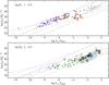 |
Fig. 6 M• weighted 5 GHz radio luminosity versus the soft X-ray luminosity in units of the Eddington luminosity (from the fundamental plane equation in Merloni et al. 2003). Symbol shapes as in Fig. 5. For clarity, our data are presented as open black squares. In addition, we show the data of Merloni et al. (2003, gray asterisks) and the low-luminosity AGN of Yuan et al. (2009, violet, downpointing triangles). The dashed violet line represents the fit of Yuan et al. (2009) adopted to soft X-rays. The thin gray line shows the fundamental plane of Merloni et al. (2003) adopted for the soft X-rays. The thin black dotted (dot-dashed) lines indicate constant RX = −1.5 (RX = −4.5) for typical log M• [M⊙] = 6 and 10 (upper and lower line), respectively. These lines have a slope of unity. Furthermore, we present data from Hardcastle et al. (2009, stars), for which the fraction of accretion related X-ray emission could be determined. The brown-colored full stars correspond to the full X-ray and the brown open stars to the accretion-related X-ray luminosities. Upper panel: presented are RL objects, RX > − 2.5, according to Panessa et al. (2007). The thick, dashed light-gray line represents the fit of Li et al. (2008) to their RL BLAGN. Lower panel: presented are RQ objects, RX ≤ − 2.5, according to Panessa et al. (2007). The thick, dashed light-gray line represents the fit of Li et al. (2008) to their RQ BLAGN. See text for details. |
Eddington parameters ordered by spectral class.
4.3.3. The fundamental plane of black-hole activity
It has been recognized that stellar-mass black holes and supermassive black holes share a common black-hole fundamental plane (FP), spanned by the three parameters X-ray luminosity, radio luminosity, and black-hole mass (e.g., Gallo et al. 2003; Merloni et al. 2003; Falcke et al. 2004): log LR = ζRXlog LX + ζRMlog M• + C. This relation (i.e., its correlation coefficients) implies a fundamental connection between radio and X-ray emission producing processes. The Merloni et al. (2003) fit gives ζRX = 0.6 ± 0.11,  , and
, and  . Currently, the FP is interpreted in the context of synchrotron emission from a jet (both in the radio and X-ray regime, e.g., Falcke et al. 2004; Yuan et al. 2009) or an advection-dominated accretion flow producing X-rays together with a jet visible in the radio (Merloni et al. 2003). There are, however, complications related to selection and observational effects (cf., Körding et al. 2006).
In Fig. 6, according to the visualization by Merloni et al. (2003, their Fig. 7), we show the black-hole-mass-weighted 5 GHz luminosities versus soft X-ray luminosities in units of Eddington luminosity. The two panels correspond to RL (log RX > − 2.5) and RQ (log RX ≤ − 2.5) AGN. Our measurements are presented as black open squares in the RQ regime and the data points follow the Merloni FP relation (thin gray line, slope ζRX = 0.6) closely. For comparison, we include the same data sets as for Fig. 5. Additionally, we show data for low-luminosity AGN (LLAGN) of Yuan et al. (2009, violet downpointing triangles) and the data set of Merloni et al. (2003, grey asterisks). The fit to the Yuan et al. (2009, dashed, thin violet line) LLAGN has a slope of ζRX = 1.2316. The thin dotted and dash-dotted gray lines correspond to constant RX = −1.5 and RX = −4.5, respectively. The upper and lower lines of each pair (dotted, dash-dotted) correspond to black-hole masses M• = 106 M⊙ and M• = 1010 M⊙, respectively. Wang et al. (2006) and Li et al. (2008) find different correlation slopes for RL (ζRX = 1.5 ± 0.08, ζRM = −0.2 ± 0.1, C = 0.05 ± 0.1) and RQ (ζRX = 0.73 ± 0.10, ζRM = 0.31 ± 0.12, C = −0.68 ± 0.07) BLAGN, which are individually different from the relation found by Merloni et al. (2003). We plot their correlations (RL, RQ) as thick dashed lines in the corresponding panel in Fig. 6. The dependence on the black-hole mass in their large sample is weak and only for RQ BLAGN with black-hole masses ≲ 107.3 M⊙ a clear positive trend is observed. Körding et al. (2006), e.g., show that the Eddington ratio is an important ingredient, with strongly sub-Eddington objects following the FP relation much tighter. Hardcastle et al. (2009) demonstrated the importance of a proper separation of accretion-related from jet-related X-ray emission. Based on X-ray spectral modeling, they found that the Merloni et al. (2003) relation lies much closer to the accretion-related X-ray luminosities of their sample. We demonstrate this finding by plotting their data, for which such a decomposition is possible. Brown filled stars represent the total X-ray luminosities, while brown open stars represent the corresponding accretion-related X-ray luminosities. It appears that the current FP reflects a relation between accretion power and jet power and not the structural properties of (relativistic) jets (Hardcastle et al. 2009). Especially, low angular resolution, broad band X-ray data are prone to mixing effects (i.e. corona, jet, warm absorber, etc.), which complicates the interpretation. This is also true for our sample, which is based on the soft X-ray RASS data. Nevertheless, Li et al. (2008) studied the relation between soft X-rays and the broad Hβ emission for their sample. They found a strong correlation and interpreted it as a signature of the accretion process. Apart from the different normalization, the slope of their correlation for RQ BLAGN is quite similar to that of Merloni et al. (2003). At least, the RQ BLAGN appear to be accretion-dominated.
As Hardcastle et al. (2009) and Yuan et al. (2009) show, a proper decomposition of the X-rays into jet- and accretion-related components introduces considerably different distributions in diagrams like Fig. 6. As soon as the sample chosen covers only a narrow range in radio loudness, this results in a “correlation” slope of unity. This is indicated by lines of log RX = const. in the figure. At this point, without a proper accretion/jet decomposition, the FP does not appear to provide new information about the radio/X-ray connection. There is certain room for scatter, as indicated by the dotted and dot-dashed lines (dotted for log RX = −1.5 and dashed for log RX = −4.5), the upper ones corresponding to M• = 106 M⊙ and the lower ones to M• = 1010 M⊙.
Similarly, because radio emission is produced by relativistic jets, Doppler boosting of the synchrotron radiation could significantly affect the observed radio flux densities, resulting in a vertical shift in the FP diagram. Li et al. (2008) investigated the influence of relativistic beaming on their BLAGN sample. They estimate the intrinsic (unbeamed) radio power with the observed X-ray luminosity through the radio/X-ray correlation derived from RQ AGN only (their Fig. 13). Typically, BLAGN have boosting factors less than 30, while in the SDSS-based BLAGN sample, factors of up 1000 (which can only be produced in BL Lac objects) are found. Nevertheless, for the majority of their sample that have factors of ≲ 100, boosting alone is not sufficient to explain the observed stronger radio powers of RL BLAGN (cf., Heinz & Merloni 2004). Though, as discussed above, using soft X-ray luminosities of the RQ AGN might introduce uncertainties in the estimation of beaming factors. All this points in a direction in which it is not straightforward to read from the distribution of data points the connection between X-ray and radio emission for given samples. In other words, the details of the sample selection and observation are essential.
Interestingly, at log LX/LEdd ≳ − 1 there appears to be a limit in the Eddington-weighted X-ray luminosity in Fig. 6 for RQ AGN. In this region, objects tend to have increased radio luminosities. This is clearly visible for the Li et al. (2008) BLAGN. As discussed by the authors, the soft X-ray luminosity likely reflects the accretion process, because of the tight correlation with the broad Balmer line luminosities. This could mean that the SMBHs are accreting most efficiently around their Eddington limit and the increased radio luminosity can then be attributed to (beamed) jet emission. Our higher angular resolution radio data together with the ROSAT data follow the same trend17. Nevertheless, we do not find indications for kpc-scale jets and we would require still higher angular resolution radio observations to associate beamed radio emission with high-brightness temperatures (cf. Doi et al. 2007).
5. Summary
We have presented 18 cm MERLIN observations of 13 intermediate-redshift X-ray bright AGN, four of which have also been studied at 18 cm with Western EVN. This work is intended to be a pilot study for investigating the energetic components (i.e., starburst vs. active nucleus) in the nuclei of such AGN at high angular resolution.
Despite the variety of spectroscopic types (SY1, NLS1, LINER, BL Lac, and passive), the 18 cm emission is essentially compact in both MERLIN (on ~500 pc scales) and EVN maps (on ~40 pc scales), with up to 50% of the lower-resolution VLA flux densities being resolved out by our interferometric observations. There are no indications for distinctive jets, except for a BL Lac object (9) and an FR-II QSO (object 11).
Based on various SFR indicators, star formation does not play a dominant role, and the compact radio emission is, therefore, most likely related to the AGN. However, we cannot discern between accretion or jet-related radio emission at this point, because of the lack of spatial and spectral resolution both in the radio and X-ray domain.
Using the soft X-ray and 5 GHz luminosities, we placed our sample objects on the fundamental plane of a black-hole activity diagram (Fig. 6). Our targets follow the general trends seen in the diagram of RQ AGN. Here we used the radio over X-ray luminosity ratio as an indicator for the radio loudness. Generally, the slope of the FP is related to a specific accretion/jet model. As discussed by several authors (e.g., Yuan et al. 2009; Hardcastle et al. 2009; Körding et al. 2006), care has to be taken when estimating accretion/jet-related X-ray and radio fluxes for individual objects based on the FP. This, on the other hand, suggests that there is no simple interpretation of the FP without a proper separation of the accretion/jet components and consideration of object types (e.g., QSO, LLAGN, radio galaxy).
Our data lie close to the relation found by Merloni et al. (2003), which describes properties of the jets rather than the accretion process. Higher angular resolution radio images at several frequencies, and hard X-ray spectra are required to study the emission processes in our sources in more detail and to better constrain their position in the fundamental plane diagram.
The eMERLIN upgrade will allow for significantly improved sensitivity for imaging (down to a noise level of a few μJy) and, correspondingly, an increased sensitivity for extended emission. On the VLBI level, the e-EVN project will provide similar improvements, but for much higher angular resolution. These advancements are instrumental to further the characterization of the relevant emission components that might determine the location of AGN in the FP.
Online material
Appendix A: Notes on individual targets
SDSS J153911.17+002600.7 (1):
this AGN is an NLS1 galaxy (Zhou et al. 2006; Williams et al. 2002). From its RASS observation, a hardness ratio of HRI = 0.46 ± 0.45 and a very soft photon index Γ = 2.8 ± 0.9 have been deduced by Williams et al. (2002). Its SDSS images exhibit some irregular structures around the nucleus. Part of this structure is a foreground star. The remaining faint features might belong to the host galaxy, or to some background galaxy. It is the radio-loudest AGN in our sample, when neglecting the two jet-dominated sources (9 and 11; see below).
SDSS J150521.92+014149.8 (2):
this NLS1 galaxy shows faint signatures of a spiral host galaxy. It also exhibits a strongly blueshifted [OIII] λ5007 emission line (by about 165 km s-1), which is commonly found in NLS1s and might be related to outflows or inflows (Boroson 2005).
SDSS J134206.57+050523.8 (3):
this is an NLS1 Nagao et al. (2001); Zhou et al. (2006) and is also a member of the Li et al. (2008) sample.
SDSS J150407.51-024816.5 (4):
this elliptical LINER galaxy is the central galaxy of the compact X-ray luminous galaxy cluster RXC J1504-0248 with one of the most massive nearby cooling cores (Böhringer et al. 2005). The black-hole mass, estimated from the [SII] line width (cf., Komossa & Xu 2007) of about 3 × 10⁷ M⊙, is somewhat less than those estimated for the brightest cluster central galaxies (108 − 9 M⊙, e.g., Rafferty et al. 2006; Fujita & Reiprich 2004).
In our MERLIN 18 cm images we detected two sources (4E[ast] and 4W[est]) at the optical position of the galaxy (Fig. 3). The two components are separated by about 0 5, which corresponds to 1750 pc at z = 0.217. In the VLA archive, we found a 3.5 cm data set at an angular resolution ( ≈ 0.25″) similar to that of our MERLIN image. Both components are detected at 3.5 cm, with Fpeak(E) = 28.78 ± 0.07 mJy and Fpeak(W) = 0.60 ± 0.07 mJy. The EVN 6 cm image recovers both components, while in the EVN 18 cm image, we only detected 4E. The 18 cm limiting peak flux density of 4W is 1.4 mJy. Figure A.1 displays the continuum spectra of 4E and 4W. The MERLIN/VLA two-point spectral index
  × log (S3.5 cm/S18 cm) is 0.42 for 4E and 2.05 for 4W. The EVN two-point spectral index
  × log (S6 cm/S18 cm) is 0.14 for 4E and < 0.58 for 4W. The eastern component has a relatively flat 18-6-3.5 cm spectrum. The western component is steeper, but flattens toward shorter wavelengths. The flat nuclear spectrum might be the result of a set of closely spaced homogeneous synchrotron components or optically thin bremsstrahlung in a disk wind (cf., Blundell & Kuncic 2007). The SDSS image of the host galaxy is regular and shows no signs of a recent merger. Together with the steep spectral index, the western component does not appear to be a companion nucleus, but rather a jet component. This is consistent with an asymmetry seen in the central X-ray brightness distribution (Fig. 9 in Böhringer et al. 2005), which might be the result of interaction between the radio jet and the hot cluster medium. More conclusions are limited because the EVN 18 cm data were hampered by bad weather. More and deeper radio data are required to study the impact of the potential radio jet onto the surrounding environment.
SDSS J010649.39+010322.4 (5):
this LINER galaxy lies at the heart of the galaxy cluster RXC J0106.8+0103 or Zw 348 (e.g., Ebeling et al. 2000; Böhringer et al. 2000). In this cluster, the AGN is expected to be a major contaminant of the overall X-ray emission (Böhringer et al. 2000). However, from the low RX and R ∗ values in Fig. 5, it can be seen that the X-rays still appear to be dominated by the cluster emission. The FIRST image reveals a slight extended emission component to the southeast in addition to the compact core (the extend parameter θFIRST ≈ 1.3), which, being barely above the noise level, could be an indication for a jet component. Our MERLIN image does not reveal any extended emission, since it might resolve out faint extended emission. This galaxy is also luminous at UV wavelengths (based on GALEX data). It lies on the boundary of between large UV luminous galaxies (UVLGs) and compact UVLGs as defined by Hoopes et al. (2007). Large UVLGs are principally normal galaxies, but are very luminous primarily because of their large size. Compact UVLGs, on the other hand, are low-mass, relatively metal-poor systems that often have disturbed morphology. These systems are characterized by intense ongoing star formation. Hoopes et al. (2007) estimated the SFR by SED fitting. SFRUV ≈ 2.4 is compatible with our FIRST estimated SFR (Table 3). Our MERLIN results show a much lower SFR, which indicates that the star formation is significantly extended throughout the host and is resolved out by the interferometer. The increasing brightness temperature at MERLIN angular resolution indicates an AGN/jet origin of the unresolved emission.
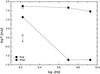 |
Fig. A.1 Target 4 radio continuum spectra of eastern and western components: MERLIN at 1.67 GHz (open symbols represent EVN measurements), EVN at 5 GHz, and VLA at 8.46 GHz. |
SDSS J074738.38+245637.3 (6):
this early-type Seyfert 1 has a companion SDSS J074738.25+245626.1 at z = 0.131. Low surface-brightness features in the SDSS images are located between the two galaxies. Gravitational interaction could therefore be responsible for the SFR of ~50 M⊙ yr-1 estimated from the large aperture data. MERLIN appears to resolve out a fraction of about 80% of the FIRST emission. The resulting SFR estimate is comparable to the [OII] one, which is about 10 M⊙ yr-1. This is the most radio-quiet source of the sample, and with the MERLIN measurement it becomes even more radio-quiet,  . The X-ray luminosity is typical for Seyfert 1 galaxies, which in turn indicates that only a small fraction of the MERLIN flux density is related to star formation, to follow the X-ray/radio correlation. MERLIN probes galactic scales of ~450 pc, while the 3′′ diameter SDSS fiber probes a region of about 7 kpc diameter. This suggests that the [OII] luminosity might be related to the extended, resolved out FIRST radio emission. Higher angular resolution radio observations are required to resolve this problem.
SDSS J030639.57+000343.1 (7):
this NLS1 has a spiral morphology. The galaxy is possibly a member of a group, with a projected distance of about 110 kpc to the nearest neighbor. It has a redshifted [OIII] λ5007 emission line (~46 km s-1), which, as discussed above, indicates a complex narrow-line region kinematics (Boroson 2005).
SDSS J081026.07+234156.1 (8):
Whalen et al. (2006) classified this AGN as an NLS1 galaxy. Its optical appearance is compact. It is the radio-faintest object in our sample. With the MERLIN measurement, it becomes the second-most radio-quiet AGN,  .
.
SDSS J162332.27+284128.7 (9):
this optically unresolved object has been classified as a BL Lac object (Plotkin et al. 2008). Owing to the absence of spectral features, no black-hole mass could be estimated. This might also be a problem for its redshift, which is taken from the SDSS database. This object is not particularly radio-loud (Fig. 5), though we are supposedly observing the jet almost face on.
SDSS J080322.48+433307.1 (10):
this SY1 galaxy shows some extremely redshifted [OIII] emission (~57 km s-1,
Boroson 2005) and is also included in the large catalogs by Wang et al. (2006) and Li et al. (2008). Owing to a nearby guide star (SDSS J080324.87+433330.1), it is also suitable for AO-assisted observations.
SDSS J080644.41+484149.2 (11):
this source is the only FRII RL QSO (de Vries et al. 2006) in our sample, having a nearby natural guide star (SDSS J080645.63+484156.6). Its optical appearance is unresolved. Although it is RL in the classical sense, the RX measurement would still result in a RQ AGN. We have only used the compact nuclear radio emission. This could mean that the 40 pc scale emission is not that strongly influenced by the jet component.
SDSS J092710.60+532731.6 (12):
this radio galaxy shows a passive, elliptical optical spectrum. It has a nearby natural guide star (SDSS J092707.09+532742.3) and is likely the brightest cluster galaxy in the Zw 2379 galaxy cluster (z = 0.205; Stott et al. 2008). Its high EVN brightness temperature underlines the AGN nature of the radio emission.
SDSS J134420.87+663717.6 (13):
IRAS 13428+6652 has been identified as Seyfert 1.5 by Moran et al. (1996). It appears to be a major merger with an extended tidal tail and possibly two nuclei. It is suitable for AO-assisted studies (SDSS J134427.10+663705.2). The source has been detected at 20 cm by NVSS. However, we could not detect any compact flux density at 18 cm with MERLIN. Since it is an IR luminous galaxy (LFIR ≈ 5 × 10¹¹ L⊙), the radio emission is most likely dominated by extended star formation.
The last four objects in Table 1 have nearby (<40″), bright (r < 15 mag) guide stars and are suitable for adaptive-optics assisted follow-up observations of their host galaxies at near-IR wavelengths (cf., Zuther et al. 2009).
For brevity, we will refer to the ID instead of the SDSS name throughout the paper.
Throughout the paper we use Fν ∝ ν − α.
Portable, Interactive Multi-Mission Simulator, Version 3.8a2.
For the energy index we used the form N(E) ∝ E − Γ, and Γ = α + 1.
ftp://ftp.astro.caltech.edu/pub/difmap/difmap.html
We use the term map in the context of the interferometric observations for the graphical representation of the reconstructed images by contours.
The measured σ values are consistent with the noise levels, as derived theoretically (cf., Wrobel & Walker 1999), using typical MERLIN system parameters.
For a typical radio spectral index (α = 0.7), the MERLIN 18 cm fluxes densities are only marginally different from the estimated 20 cm ones.
Take, for example, the ULIG 3C 48, which has a similar redshift and infrared luminosity (z = 0.3695, LIR ≈ 5 × 10¹² L⊙) and has been clearly detected with IRAS (Neugebauer et al. 1985).
Here, a certain amount of caution is advisable, because it is currently unclear whether soft (0.1 − 2 keV) and hard X-rays (2 − 10 keV) have the same origin for the various classes of objects presented in Figs. 5 and 6. Furthermore, soft 0.1 − 2.4 keV X-rays are more prone to extinction than the harder 2 − 10 keV X-rays.
Based on the width of their broad Hβ lines and the broad-line-region radius luminosity relation from Bentz et al. (2009).
Actually, the optical luminosity density used in Vestergaard (2004) is measured at 4400 Å. Arguably, the commonly used luminosity density at 5100 Å is sufficiently close in wavelength to yield consistent values.
Yuan et al. (2009) found the following correlation coefficients: ζRX = 1.22, ζRM = 0.23, C = −12.46.
This takes into account the similar database (i.e., SDSS/ROSAT/ FIRST matches).
Acknowledgments
The authors kindly thank the anonymous referee for fruitful comments and suggestions. The authors kindly thank Anita Richards, Tom Muxlow, and Giuseppe Cimo for their help during data reduction, as well as Martin Hardcastle for kindly providing additional information on their X-ray study of 3CRR sources. This work has benefited from research funding from the European Community’s sixth Framework Programme under RadioNet R113CT 2003 5058187. MERLIN is a National Facility operated by the University of Manchester at Jodrell Bank Observatory on behalf of STFC. The European VLBI Network is a joint facility of European, Chinese, South African and other radio astronomy institutes funded by their national research councils. Part of this work was supported by the German Deutsche Forschungsgemeinschaft, DFG project numbers SFB 494 and SFB 956. J.Z. acknowledges support from the European project EuroVO DCA under the Research e-Infrastructures area (RI031675).
References
- Abazajian, K., Adelman-McCarthy, J. K., Agüeros, M. A., et al. 2004, AJ, 128, 502 [Google Scholar]
- Anderson, S. F., Voges, W., Margon, B., et al. 2003, AJ, 126, 2209 [NASA ADS] [CrossRef] [Google Scholar]
- Anderson, S. F., Margon, B., Voges, W., et al. 2007, AJ, 133, 313 [NASA ADS] [CrossRef] [Google Scholar]
- Balmaverde, B., & Capetti, A. 2006, A&A, 447, 97 [NASA ADS] [CrossRef] [EDP Sciences] [Google Scholar]
- Barai, P., Proga, D., & Nagamine, K. 2011, MNRAS, in press [arXiv:1112.5483] [Google Scholar]
- Barvainis, R., & Lonsdale, C. 1997, AJ, 113, 144 [NASA ADS] [CrossRef] [Google Scholar]
- Barvainis, R., Lonsdale, C., & Antonucci, R. 1996, AJ, 111, 1431 [NASA ADS] [CrossRef] [Google Scholar]
- Becker, R. H., White, R. L., & Helfand, D. J. 1995, ApJ, 450, 559 [NASA ADS] [CrossRef] [Google Scholar]
- Bell, E. F. 2003, ApJ, 586, 794 [Google Scholar]
- Bentz, M. C., Peterson, B. M., Netzer, H., Pogge, R. W., & Vestergaard, M. 2009, ApJ, 697, 160 [Google Scholar]
- Bian, W., & Zhao, Y. 2004, MNRAS, 352, 823 [NASA ADS] [CrossRef] [Google Scholar]
- Blundell, K. M., & Beasley, A. J. 1998, MNRAS, 299, 165 [NASA ADS] [CrossRef] [Google Scholar]
- Blundell, K. M., & Kuncic, Z. 2007, ApJ, 668, L103 [NASA ADS] [CrossRef] [Google Scholar]
- Blustin, A. J., Dwelly, T., Page, M. J., et al. 2008, MNRAS, 390, 1229 [NASA ADS] [CrossRef] [Google Scholar]
- Böhringer, H., Voges, W., Huchra, J. P., et al. 2000, ApJS, 129, 435 [NASA ADS] [CrossRef] [Google Scholar]
- Böhringer, H., Burwitz, V., Zhang, Y., Schuecker, P., & Nowak, N. 2005, ApJ, 633, 148 [NASA ADS] [CrossRef] [Google Scholar]
- Boroson, T. 2005, AJ, 130, 381 [NASA ADS] [CrossRef] [Google Scholar]
- Brandt, W. N., & Hasinger, G. 2005, ARA&A, 43, 827 [Google Scholar]
- Bridle, A. H., & Perley, R. A. 1984, ARA&A, 22, 319 [NASA ADS] [CrossRef] [Google Scholar]
- Brinkmann, W., Laurent-Muehleisen, S. A., Voges, W., et al. 2000, A&A, 356, 445 [NASA ADS] [Google Scholar]
- Cirasuolo, M., Celotti, A., Magliocchetti, M., & Danese, L. 2003, MNRAS, 346, 447 [NASA ADS] [CrossRef] [Google Scholar]
- Condon, J. J. 1992, ARA&A, 30, 575 [NASA ADS] [CrossRef] [MathSciNet] [Google Scholar]
- Condon, J. J., & Yin, Q. F. 1990, ApJ, 357, 97 [NASA ADS] [CrossRef] [Google Scholar]
- Condon, J. J., Condon, M. A., Gisler, G., & Puschell, J. J. 1982, ApJ, 252, 102 [NASA ADS] [CrossRef] [Google Scholar]
- Condon, J. J., Anderson, M. L., & Helou, G. 1991, ApJ, 376, 95 [NASA ADS] [CrossRef] [Google Scholar]
- Cotton, W. D., Wittels, J. J., Shapiro, I. I., et al. 1980, ApJ, 238, L123 [NASA ADS] [CrossRef] [Google Scholar]
- David, L. P., Jones, C., & Forman, W. 1992, ApJ, 388, 82 [NASA ADS] [CrossRef] [Google Scholar]
- de Vries, W. H., Becker, R. H., & White, R. L. 2006, AJ, 131, 666 [NASA ADS] [CrossRef] [Google Scholar]
- Dickey, J. M., & Lockman, F. J. 1990, ARA&A, 28, 215 [NASA ADS] [CrossRef] [MathSciNet] [Google Scholar]
- Doi, A., Fujisawa, K., Inoue, M., et al. 2007, PASJ, 59, 703 [NASA ADS] [Google Scholar]
- Draine, B. T. 2011, Physics of the Interstellar and Intergalactic Medium (Princeton University Press) [Google Scholar]
- Dudik, R. P., Satyapal, S., Gliozzi, M., & Sambruna, R. M. 2005, ApJ, 620, 113 [NASA ADS] [CrossRef] [Google Scholar]
- Ebeling, H., Edge, A. C., Allen, S. W., et al. 2000, MNRAS, 318, 333 [NASA ADS] [CrossRef] [Google Scholar]
- Falcke, H., Körding, E., & Markoff, S. 2004, A&A, 414, 895 [NASA ADS] [CrossRef] [EDP Sciences] [Google Scholar]
- Fujita, Y., & Reiprich, T. H. 2004, ApJ, 612, 797 [NASA ADS] [CrossRef] [Google Scholar]
- Gallo, E., Fender, R. P., & Pooley, G. G. 2003, MNRAS, 344, 60 [NASA ADS] [CrossRef] [Google Scholar]
- Greene, J. E., & Ho, L. C. 2007, ApJ, 667, 131 [NASA ADS] [CrossRef] [Google Scholar]
- Grupe, D., Wills, B. J., Leighly, K. M., & Meusinger, H. 2004, AJ, 127, 156 [NASA ADS] [CrossRef] [Google Scholar]
- Haardt, F., & Maraschi, L. 1991, ApJ, 380, L51 [NASA ADS] [CrossRef] [Google Scholar]
- Hamilton, T. S. 2010, MNRAS, 1111 [Google Scholar]
- Hardcastle, M. J., Evans, D. A., & Croston, J. H. 2009, MNRAS, 396, 1929 [NASA ADS] [CrossRef] [Google Scholar]
- Heckman, T. M. 1980, A&A, 87, 152 [NASA ADS] [Google Scholar]
- Heinz, S., & Merloni, A. 2004, MNRAS, 355, L1 [NASA ADS] [CrossRef] [Google Scholar]
- Hill, T. L., Heisler, C. A., Norris, R. P., Reynolds, J. E., & Hunstead, R. W. 2001, AJ, 121, 128 [NASA ADS] [CrossRef] [Google Scholar]
- Ho, L. C. 2005, ApJ, 629, 680 [NASA ADS] [CrossRef] [Google Scholar]
- Ho, L. C. 2008, ARA&A, 46, 475 [NASA ADS] [CrossRef] [Google Scholar]
- Ho, L. C., & Peng, C. Y. 2001, ApJ, 555, 650 [NASA ADS] [CrossRef] [Google Scholar]
- Hoopes, C. G., Heckman, T. M., Salim, S., et al. 2007, ApJS, 173, 441 [NASA ADS] [CrossRef] [Google Scholar]
- Hopkins, A. M., Miller, C. J., Nichol, R. C., et al. 2003, ApJ, 599, 971 [NASA ADS] [CrossRef] [Google Scholar]
- Ivezić, Ž., Menou, K., Knapp, G. R., et al. 2002, AJ, 124, 2364 [NASA ADS] [CrossRef] [Google Scholar]
- Jakobsen, P., de Vries, J. S., & Paresce, F. 1987, A&A, 183, 335 [NASA ADS] [Google Scholar]
- Kaspi, S., Maoz, D., Netzer, H., et al. 2005, ApJ, 629, 61 [NASA ADS] [CrossRef] [Google Scholar]
- Kellermann, K. I., & Pauliny-Toth, I. I. K. 1969, ApJ, 155, L71 [NASA ADS] [CrossRef] [Google Scholar]
- Kellermann, K. I., Sramek, R., Schmidt, M., Shaffer, D. B., & Green, R. 1989, AJ, 98, 1195 [NASA ADS] [CrossRef] [Google Scholar]
- Kennicutt, Jr., R. C. 1998, ARA&A, 36, 189 [Google Scholar]
- Komossa, S., & Xu, D. 2007, ApJ, 667, L33 [NASA ADS] [CrossRef] [Google Scholar]
- Körding, E., Falcke, H., & Corbel, S. 2006, A&A, 456, 439 [NASA ADS] [CrossRef] [EDP Sciences] [Google Scholar]
- Krips, M., Eckart, A., Krichbaum, T. P., et al. 2007, A&A, 464, 553 [NASA ADS] [CrossRef] [EDP Sciences] [Google Scholar]
- Laine, S., Kotilainen, J. K., Reunanen, J., Ryder, S. D., & Beck, R. 2006, AJ, 131, 701 [NASA ADS] [CrossRef] [Google Scholar]
- Laor, A., & Behar, E. 2008, MNRAS, 390, 847 [NASA ADS] [CrossRef] [Google Scholar]
- Leipski, C., Falcke, H., Bennert, N., & Hüttemeister, S. 2006, A&A, 455, 161 [NASA ADS] [CrossRef] [EDP Sciences] [Google Scholar]
- Li, Z., Wu, X., & Wang, R. 2008, ApJ, 688, 826 [NASA ADS] [CrossRef] [Google Scholar]
- Linsky, J. L., Rickett, B. J., & Redfield, S. 2008, ApJ, 675, 413 [NASA ADS] [CrossRef] [Google Scholar]
- Mannucci, F., Maiolino, R., Cresci, G., et al. 2003, A&A, 401, 519 [NASA ADS] [CrossRef] [EDP Sciences] [Google Scholar]
- Merloni, A., Heinz, S., & di Matteo, T. 2003, MNRAS, 345, 1057 [NASA ADS] [CrossRef] [Google Scholar]
- Miller, B. P., Brandt, W. N., Gibson, R. R., Garmire, G. P., & Shemmer, O. 2009, ApJ, 702, 911 [NASA ADS] [CrossRef] [Google Scholar]
- Moran, E. C., Halpern, J. P., & Helfand, D. J. 1996, ApJS, 106, 341 [NASA ADS] [CrossRef] [Google Scholar]
- Muxlow, T. W. B., Pedlar, A., Wilkinson, P. N., et al. 1994, MNRAS, 266, 455 [NASA ADS] [CrossRef] [Google Scholar]
- Nagao, T., Murayama, T., & Taniguchi, Y. 2001, ApJ, 546, 744 [NASA ADS] [CrossRef] [Google Scholar]
- Narayan, R., Mahadevan, R., & Quataert, E. 1998, in Theory of Black Hole Accretion Disks, ed. M. A. Abramowicz, G. Bjornsson, & J. E. Pringle, 148 [Google Scholar]
- Neugebauer, G., Soifer, B. T., & Miley, G. K. 1985, ApJ, 295, L27 [NASA ADS] [CrossRef] [Google Scholar]
- Panessa, F., Wolter, A., Pellegrini, S., et al. 2005, ApJ, 631, 707 [NASA ADS] [CrossRef] [Google Scholar]
- Panessa, F., Bassani, L., Cappi, M., et al. 2006, A&A, 455, 173 [NASA ADS] [CrossRef] [EDP Sciences] [Google Scholar]
- Panessa, F., Barcons, X., Bassani, L., et al. 2007, A&A, 467, 519 [NASA ADS] [CrossRef] [EDP Sciences] [Google Scholar]
- Perola, G. C., Matt, G., Cappi, M., et al. 2002, A&A, 389, 802 [Google Scholar]
- Peterson, B. M. 1997, An Introduction to Active Galactic Nuclei (Cambridge University Press) [Google Scholar]
- Plotkin, R. M., Anderson, S. F., Hall, P. B., et al. 2008, AJ, 135, 2453 [NASA ADS] [CrossRef] [Google Scholar]
- Quirrenbach, A., Witzel, A., Kirchbaum, T. P., et al. 1992, A&A, 258, 279 [NASA ADS] [Google Scholar]
- Rafferty, D. A., McNamara, B. R., Nulsen, P. E. J., & Wise, M. W. 2006, ApJ, 652, 216 [NASA ADS] [CrossRef] [Google Scholar]
- Readhead, A. C. S. 1994, ApJ, 426, 51 [Google Scholar]
- Salvato, M., Greiner, J., & Kuhlbrodt, B. 2004, ApJ, 600, L31 [NASA ADS] [CrossRef] [Google Scholar]
- Sanders, D. B., & Mirabel, I. F. 1996, ARA&A, 34, 749 [NASA ADS] [CrossRef] [Google Scholar]
- Schneider, D. P., Fan, X., Hall, P. B., et al. 2003, AJ, 126, 2579 [NASA ADS] [CrossRef] [Google Scholar]
- Schulze, A., Wisotzki, L., & Husemann, B. 2009, A&A, 507, 781 [NASA ADS] [CrossRef] [EDP Sciences] [Google Scholar]
- Shepherd, M. C. 1997, in Astronomical Data Analysis Software and Systems VI, ed. G. Hunt, & H. Payne, ASP Conf. Ser., 125, 77 [Google Scholar]
- Shields, G. A. 1978, Nature, 272, 706 [NASA ADS] [CrossRef] [Google Scholar]
- Sikora, M., Stawarz, Ł., & Lasota, J.-P. 2007, ApJ, 658, 815 [NASA ADS] [CrossRef] [Google Scholar]
- Spergel, D. N., Verde, L., Peiris, H. V., et al. 2003, ApJS, 148, 175 [NASA ADS] [CrossRef] [Google Scholar]
- Steenbrugge, K. C., Jolley, E. J. D., Kuncic, Z., & Blundell, K. M. 2011, MNRAS, 413, 1735 [NASA ADS] [CrossRef] [Google Scholar]
- Stott, J. P., Edge, A. C., Smith, G. P., Swinbank, A. M., & Ebeling, H. 2008, MNRAS, 384, 1502 [NASA ADS] [CrossRef] [Google Scholar]
- Terashima, Y., & Wilson, A. S. 2003, ApJ, 583, 145 [NASA ADS] [CrossRef] [Google Scholar]
- Terlevich, R., Tenorio-Tagle, G., Franco, J., & Melnick, J. 1992, MNRAS, 255, 713 [NASA ADS] [CrossRef] [Google Scholar]
- Ulvestad, J. S., Antonucci, R. R. J., & Barvainis, R. 2005, ApJ, 621, 123 [NASA ADS] [CrossRef] [Google Scholar]
- Vitale, et al. 2012, A&A, submitted [Google Scholar]
- Vestergaard, M. 2004, ApJ, 601, 676 [NASA ADS] [CrossRef] [Google Scholar]
- Villar-Martín, M., Humphrey, A., Martínez-Sansigre, A., et al. 2008, MNRAS, 390, 218 [NASA ADS] [CrossRef] [Google Scholar]
- Voges, W., Aschenbach, B., Boller, T., et al. 1999, A&A, 349, 389 [NASA ADS] [Google Scholar]
- Wang, R., Wu, X., & Kong, M. 2006, ApJ, 645, 890 [NASA ADS] [CrossRef] [Google Scholar]
- Weiler, K. W., Panagia, N., & Sramek, R. A. 1990, ApJ, 364, 611 [NASA ADS] [CrossRef] [Google Scholar]
- Wells, D. C. 1985, in Data Analysis in Astronomy, ed. V. di Gesu, L. Scarsi, P. Crane, J. H. Friedman, & S. Levialdi, 195 [Google Scholar]
- Whalen, D. J., Laurent-Muehleisen, S. A., Moran, E. C., & Becker, R. H. 2006, AJ, 131, 1948 [NASA ADS] [CrossRef] [Google Scholar]
- Williams, R. J., Pogge, R. W., & Mathur, S. 2002, AJ, 124, 3042 [NASA ADS] [CrossRef] [Google Scholar]
- Wrobel, J. M., & Walker, R. C. 1999, in Synthesis Imaging in Radio Astronomy II, ed. G. B. Taylor, C. L. Carilli, & R. A. Perley, ASP Conf. Ser., 180, 171 [Google Scholar]
- Wu, X., & Liu, F. K. 2004, ApJ, 614, 91 [NASA ADS] [CrossRef] [Google Scholar]
- Yuan, F., Cui, W., & Narayan, R. 2005, ApJ, 620, 905 [NASA ADS] [CrossRef] [Google Scholar]
- Yuan, F., Yu, Z., & Ho, L. C. 2009, ApJ, 703, 1034 [NASA ADS] [CrossRef] [Google Scholar]
- Zhou, H., Wang, T., Yuan, W., et al. 2006, ApJS, 166, 128 [NASA ADS] [CrossRef] [Google Scholar]
- Zuther, J. 2007, Ph.D. Thesis, University of Cologne [Google Scholar]
- Zuther, J., Lemson, G., Eckart, A., et al. 2009, in Multi-wavelength Astronomy and Virtual Observatory, ed. D. Baines, & P. Osuna, 15 [Google Scholar]
All Tables
MERLIN, EVN measurements, basic source parameters, and derived brightness temperatures, star-formation rates.
All Figures
|
Fig. 1 0.1−2.4 keV X-ray vs. 20 cm FIRST peak luminosity. Symbols of our sources are indicated in the legend and correspond to spectroscopic types. Colors are coded according to the black-hole mass. Open symbols are for objects without available black-hole mass. For comparison, we present SDSS/FIRST/ROSAT-based broad-line AGN (BLAGN) from Li et al. (2008, × correspond to RQ and +. The dashed line is the linear correlation for RQ QSO of Brinkmann et al. (2000). |
| In the text | |
|
Fig. 2 Maps of the MERLIN 18 cm reconstructed images of the detected sources (detection threshold 3σ). Contours refer to − 2 (dashed), 2, 3, 4, 5, and 6 times the σ in the image. Except for sources 7 and 9, for which the contours refer to −2, 2, 3, 4, 8, 16, 32, ... times the σ. All σ values are given in Table 3. The beams are indicated in the bottom left corner of the maps. North is up, East is left. Sources with EVN follow-up observations are shown in Fig. 3. |
| In the text | |
|
Fig. 3 The first two columns present MERLIN and EVN 18 cm reconstructed maps. The third column shows the MERLIN 18 cm map of source 4 in the first row. The second row shows the EVN 6 cm map including the eastern and western components. In the third row we present a close-up of the eastern component in the EVN 18 cm map. The western component was not detected. We present maps of the cleaned images of the detected sources (detection threshold 3σ). Contours refer to − 3 (dashed), 3, 4, 8, 16, ... times the σ in the images. The σ values are given in Table 3. The beams are indicated in the bottom left corner of the maps. North is up, East is left. |
| In the text | |
|
Fig. 4 Brightness temperature vs. star-formation rate, both estimated from radio flux densities. The symbol size corresponds to the source size of the individual observation. FIRST, MERLIN, and EVN measurements of each source are connected by a line. General symbol shapes as in Fig. 1. |
| In the text | |
|
Fig. 5 Radio/X-ray vs. radio/optical flux ratio. Diagonal lines indicate optical/X-ray ratios of 1, 10, and 100. Symbol shapes as in Fig. 1. Black symbols are based on our MERLIN measurements. The black open right triangle corresponds to the radio upper-limit-based values of source 13. Red symbols are based on our EVN measurements. The open magenta triangles are data from Ulvestad et al. (2005). Green hexagons are low-luminosity Seyfert 1, 2 galaxies from Panessa et al. (2007), blue crosses radio galaxies from Balmaverde & Capetti (2006). Cyan diamonds are soft X-ray selected NLS1s from Grupe et al. (2004). Light gray plus signs are BLAGN from Li et al. (2008). Japanese VLBI observations of two of them are represented by orange pentagons (Doi et al. 2007). Note that only our data and those of Ulvestad et al. and Doi et al. are based on high angular resolution radio observations. The dotted horizontal and vertical lines mark the refined RL/RQ demarcation from Panessa et al. (2007). |
| In the text | |
|
Fig. 6 M• weighted 5 GHz radio luminosity versus the soft X-ray luminosity in units of the Eddington luminosity (from the fundamental plane equation in Merloni et al. 2003). Symbol shapes as in Fig. 5. For clarity, our data are presented as open black squares. In addition, we show the data of Merloni et al. (2003, gray asterisks) and the low-luminosity AGN of Yuan et al. (2009, violet, downpointing triangles). The dashed violet line represents the fit of Yuan et al. (2009) adopted to soft X-rays. The thin gray line shows the fundamental plane of Merloni et al. (2003) adopted for the soft X-rays. The thin black dotted (dot-dashed) lines indicate constant RX = −1.5 (RX = −4.5) for typical log M• [M⊙] = 6 and 10 (upper and lower line), respectively. These lines have a slope of unity. Furthermore, we present data from Hardcastle et al. (2009, stars), for which the fraction of accretion related X-ray emission could be determined. The brown-colored full stars correspond to the full X-ray and the brown open stars to the accretion-related X-ray luminosities. Upper panel: presented are RL objects, RX > − 2.5, according to Panessa et al. (2007). The thick, dashed light-gray line represents the fit of Li et al. (2008) to their RL BLAGN. Lower panel: presented are RQ objects, RX ≤ − 2.5, according to Panessa et al. (2007). The thick, dashed light-gray line represents the fit of Li et al. (2008) to their RQ BLAGN. See text for details. |
| In the text | |
|
Fig. A.1 Target 4 radio continuum spectra of eastern and western components: MERLIN at 1.67 GHz (open symbols represent EVN measurements), EVN at 5 GHz, and VLA at 8.46 GHz. |
| In the text | |
Current usage metrics show cumulative count of Article Views (full-text article views including HTML views, PDF and ePub downloads, according to the available data) and Abstracts Views on Vision4Press platform.
Data correspond to usage on the plateform after 2015. The current usage metrics is available 48-96 hours after online publication and is updated daily on week days.
Initial download of the metrics may take a while.