© ESO, 2012

1. Introduction

The everyday experience of velocity shear in a fluid flow is that if the shear is large enough a laminar flow will become turbulent. In non-rotating flow such as Poiseiulle flow or plane-Couette flow the laminar state is linearly stable at all Reynolds numbers. Nevertheless, in the presence of disturbances of finite amplitude, a transition to turbulence can occur (Darbyshire & Mullin 1994). In the case of rotating shear flow, such as the Taylor-Couette flow (Taylor 1923; Couette 1888) established between concentric rotating cylinders, a transition to turbulence was observed (Wendt 1933; Taylor 1936) for the case in which the inner cylinder was at rest with the outer one spinning. This configuration is linearly stable to infinitesimal perturbations at all Reynolds numbers. Nevertheless, instability was observed at Re ~ 10³ − 10⁵. The transition has been assumed to be subcritical due to similarities with pipe flow transition, though Schultz-Grunow (1959) stated that the transition appeared to be similar to a Kelvin-Helmholtz instability. No first-principles theory exists for subcritical transition in a rotating shear flow, though recent efforts to identify such a transition mechanism can be found in Chagelishvili et al. (2003); Tevzadze et al. (2003); Yecko (2004); Umurhan & Regev (2004); Mukhopadhyay et al. (2005); Afshordi et al. (2005); Lithwick (2007); Rincon et al. (2007); Lithwick (2009); Mukhopadhyay et al. (2011); Mukhopadhyay & Saha (2011). Phenomenological models have been developed based on the assumption that the observed transition is subcritical in nature (Zeldovich 1981; Richard & Zahn 1999; Longaretti 2002; Dubrulle et al. 2005).

Fig. 1 Rotation profiles developed between concentric, co-rotating cylinders. The axes are the rotation speeds of the cylinders defined by a Reynolds number Re1,2 = Ω1,2r1,2(r2 − r1)/ν, where 1 (2) refers to the inner (outer) cylinder. The cylinder radius is r and Ω is the angular velocity. The kinematic viscosity is ν. The flow profiles are classified by a local exponent of angular velocity q ≡ − ∂lnΩ/∂lnr. In cyclonic flow q < 0. The anti-cyclonic regime is further divided in to quasi-Keplerian and centrifugally unstable flows, the boundary between the two is the flat angular momentum profile, q = 2.

This observation has motivated hydrodynamic theories of accretion mechanisms since the work of Shakura & Sunyaev (1973). The linear magnetorotational instability (MRI) (Balbus & Hawley 1991) has since emerged as the mechanism most likely to provide the required levels of angular momentum transport. However, the electrical conductivity of protostellar accretion disks is at best marginally adequate for MRI-driven accretion (Bai 2011; Oishi & Mac Low 2011) and references therein. Therefore, purely hydrodynamic models based on subcritical hydrodynamic instability (SHI) still remain of interest for these cool disks.

A review of transport mechanisms in accretion disks can be found in Balbus & Hawley (1998). The matter in thin accretion disks follow Keplerian angular velocity profiles, Ω(r) ∝ r ^− 3/2, the angular momentum increases with radius, l(r) ∝ r²Ω ∝ r^1/2 and the disk is stable to linear centrifugal instability (Rayleigh 1916). In SHI models of disk accretion, shear in the angular velocity is the source of free energy to drive enhanced transport. A dimensionless coefficient β relates the shear to a turbulent viscosity, ν_T. Modeling by Hueso & Guillot (2005) of two protoplanetary systems require that β lies in the range 10^-6 − 10^-4, which appears to be compatible with the deduced β by Richard & Zahn (1999) based on the Taylor-Couette flow experiments by Wendt (1933) and Taylor (1936).

The velocity profile developed in a Taylor-Couette experiment may share with the Keplerian flow the opposing gradients of angular momentum and angular velocity. We refer to these flows as quasi-Keplerian. The quasi-Keplerian profile is a subset of anti-cyclonic profiles in which ∂Ω/∂r < 0 and may be either centrifugally unstable, ∂l/∂r < 0, or stable, ∂l/∂r > 0. Flows in which ∂Ω/∂r > 0 are cyclonic and are linearly stable at all Reynolds numbers. This is the regime in which Wendt and Taylor made their observations. It is worth noting that the β prescription by Richard & Zahn (1999), even if valid for the cyclonic evidence on which they based it, may not be valid for anti-cyclonic flow, in particular Keplerian flow.

The Princeton MRI experiment is a Taylor-Couette device developed (Schartman et al. 2009) to produce quasi-Keplerian flows in both water and a liquid gallium alloy to look for evidence of both SHI using water and the MRI using alloy (Ji et al. 2001; Goodman & Ji 2002). The flows of interest are diagrammed in Fig. 1. We use two dimensionless numbers to characterize our flow profiles: the Reynolds number, Re, and the local exponent of angular velocity, q. The concentric cylinders have radii r₁,r₂ (r₁ < r₂) and angular velocities Ω₁,Ω₂. We define $\mathit{Re}\mathrm{\equiv }\left({\mathrm{\Omega }}_{\mathrm{1}}\mathrm{-}{\mathrm{\Omega }}_{\mathrm{2}}\right){}^{\mathrm{(}}\mathit{r}_{\mathrm{2}}\mathrm{-}{\mathit{r}}_{\mathrm{1}}{}^{\mathrm{)}}\mathit{r̅}\mathit{/}\mathit{\nu }$, where and ν is the kinematic viscosity. We follow the definition used in Balbus & Hawley (1998) for q ≡ − ∂lnΩ/∂lnr. For a Keplerian disk q = 3/2, and the limit of marginal stability by the Rayleigh criterion occurs for q = 2.

Based on observations of SHI in non-rotating flow three characteristics are always present. 1) The laminar state before transition is linearly stable to infinitesimal perturbations. 2) A hysteresis is observed in the transition: the change from the laminar to the turbulent state occurs at a greater Reynolds number than the transition from turbulent to laminar flow. 3) The transition to the turbulent state is triggered by the presence of ambient fluctuations in the laminar flow. For circular Poiseuille flow no transition occurs below Re ≈ 2 × 10³, even for perturbation amplitude equal to the mean flow velocity (Darbyshire & Mullin 1994). At higher Reynolds number, the fluctuation level required to trigger transition decreases. In carefully controlled experiments the transition has been delayed to Re ~ 10⁵ (Pfenniger 1961).

Local shearing box simulations have been performed to investigate the hydrodynamic stability of quasi-Keplerian flows. Hawley et al. (1999) and Lesur & Longaretti (2005) studied the decay of applied turbulence near the boundary of marginal centrifugal instability (Rayleigh 1916). Both investigations excite transiently the largest Fourier modes of the simulation domain and observe the subsequent evolution of the flow. In both simulations the turbulence decays rapidly for all quasi-Keplerian values of q, except those close to centrifugal instability. Hawley et al. (1999) report that for q/2 < 99.5% and perturbation amplitudes of v′/v = 1 to 100% the flow relaminarizes within one to five orbital periods.

In the anti-cyclonic cases investigated by Lesur & Longaretti (2005) they begin the simulation on the marginally-centrifugally stable boundary, q = 2, with a perturbation amplitude of 100%. While holding Re constant, they gradually step in to the centrifugally stable regime until the flow becomes laminar. They observe that the turbulence persists into the stable regime, but that the critical Reynolds number is an extremely steep function of the distance to the linear stability boundary. In going from q/2 ≈ 99% to q/2 ≈ 97%, the transition Reynolds number increases from  < 1 × 10⁴ to  ≈ 8 × 10⁴.

The forcing amplitude imposed on a fully developed flow used by Lesur & Longaretti (2005) cannot be produced in the Princeton MRI Experiment. We are restricted to forcing the flow with ambient fluctuation levels generated by the boundaries, or by accelerating the boundaries to produce a new flow profile. In the latter case, a statistically steady mean velocity is not reached before the fluctuation levels fall below 5%. In the most unstable flows which we can produce via instability, the maximum measured fluctuation amplitude is of order 10%. No apparent hystereses associated with a transition were observed with these attempts.

Prior to our work in this regime, Richard (2001) and Beckley (2002) were the only experiments to study the stability of quasi-Keplerian flows. Richard’s experiments were performed at Re ~ 10⁴, and Beckley’s were at Re ~ 10⁶. The relation of these Reynolds numbers to our experiments are shown in Fig. 1. Beckley diagnosed his flow by measuring the torque required to maintain a steady state flow. He found that the Reynolds number scaling of this torque was inconsistent with laminar Taylor-Couette flow. Beckley’s apparatus was constructed with cylinder heights comparable to the gap between them, h = 2(r₂ − r₁), and the end caps fixed to the outer cylinder. Because of the relative proximity of the end caps and their speed, Beckley concluded that the excess torque was due to an Ekman circulation (see Sect. 3.4).

The Taylor-Couette device employed by Richard (2001) used taller cylinders, h ≈ 25(r₂ − r₁), with less influence on the bulk flow from the end caps than Beckley’s apparatus (by using a “split” configuration; see Sect. 3 below). Using a visualization technique, Richard observed that his flow underwent a transition to wavy states (Longaretti 2008, priv. comm.) at a Reynolds number of approximately 10⁴, but without quantitative measurements of the angular momentum transport. The measured profiles of the mean azimuthal velocity, however, still deviated significantly from the ideal Couette solution (see Sect. 2 below), presumably due to Ekman circulation driven by the endcaps.

In this paper we present the results of our investigation of SHI in quasi-Keplerian flows in the Princeton MRI experiment. We show significant influences by end caps on the measured angular momentum transport. By using two independently rotatable end caps at each end, the Ekman effects are minimized, resulting in much lower transport levels than proposed by Richard & Zahn (1999). The implications to angular momentum transport in astrophysical disks are discussed.

2. Measurement of angular momentum transport

We briefly review the hydrodynamics of the ideal Couette flow to make explicit the terms which are accessible experimentally to us. We work in cylindrical coordinates (r,θ,z). The incompressible Navier-Stokes equations with stress tensor $\overline{\mathit{\sigma }}$ are: $\begin{array}{ccc}\frac{\mathit{\partial }{v}}{\mathit{\partial t}}\mathrm{+}\left({v}\mathrm{·}\mathrm{\nabla }\right){v}& \mathrm{=}& \mathrm{\nabla }\mathrm{·}\overline{\mathit{\sigma }}\\ \mathrm{\nabla }\mathrm{·}{v}& \mathrm{=}& \mathrm{0.}\end{array}$Writing out the full equation for the azimuthal velocity, v_θ: $\begin{array}{ccc}\frac{\mathit{\partial }{\mathit{v}}_{\mathit{\theta }}}{\mathit{\partial t}}& \mathrm{+}& \frac{{\mathit{v}}_{\mathit{r}}}{\mathit{r}}\frac{\mathit{\partial }\mathrm{\left(}\mathit{r}{\mathit{v}}_{\mathit{\theta }}\mathrm{\right)}}{\mathit{\partial r}}\mathrm{+}\frac{{\mathit{v}}_{\mathit{\theta }}}{\mathit{r}}\frac{\mathit{\partial }{\mathit{v}}_{\mathit{\theta }}}{\mathit{\partial \theta }}\mathrm{+}{\mathit{v}}_{\mathit{z}}\frac{\mathit{\partial }{\mathit{v}}_{\mathit{\theta }}}{\mathit{\partial z}}\mathrm{=}\mathrm{-}\frac{\mathrm{1}}{\mathit{\rho r}}\frac{\mathit{\partial p}}{\mathit{\partial \theta }}\\ & & \end{array}$(3)For steady-state, laminar flow where the transport is only radial (i.e. infinitely tall cylinders), ∂/∂θ = ∂/∂z = 0, the incompressibility condition gives (1/r)∂(rv_r)/∂r = 0 and therefore v_r = 0 from the impermeable radial boundary conditions. Equation (3) becomes: $\mathrm{0}\mathrm{=}\frac{\mathrm{1}}{{\mathit{r}}^{\mathrm{2}}}\frac{\mathit{\partial }}{\mathit{\partial r}}\left[{\mathit{r}}^{\mathrm{3}}\frac{\mathit{\partial }}{\mathit{\partial r}}\left(\frac{{\mathit{v}}_{\mathit{\theta }}}{\mathit{r}}\right)\right]$(4)leading to the ideal Couette solution for the angular velocity: $\mathrm{\Omega }\mathrm{\left(}\mathit{r}\mathrm{\right)}\mathrm{=}\mathit{a}\mathrm{+}\frac{\mathit{b}}{{\mathit{r}}^{\mathrm{2}}}\mathit{,}$with constants: $\mathit{a}\mathrm{=}\frac{{\mathrm{\Omega }}_{\mathrm{2}}{\mathit{r}}_{\mathrm{2}}^{\mathrm{2}}\mathrm{-}{\mathrm{\Omega }}_{\mathrm{1}}{\mathit{r}}_{\mathrm{1}}^{\mathrm{2}}}{{\mathit{r}}_{\mathrm{2}}^{\mathrm{2}}\mathrm{-}{\mathit{r}}_{\mathrm{1}}^{\mathrm{2}}}\mathit{,} \mathit{b}\mathrm{=}\frac{\left({\mathrm{\Omega }}_{\mathrm{1}}\mathrm{-}{\mathrm{\Omega }}_{\mathrm{2}}\right){\mathit{r}}_{\mathrm{2}}^{\mathrm{2}}{\mathit{r}}_{\mathrm{1}}^{\mathrm{2}}}{{\mathit{r}}_{\mathrm{2}}^{\mathrm{2}}\mathrm{-}{\mathit{r}}_{\mathrm{1}}^{\mathrm{2}}}\mathit{,}$(5)where Ω₁ (Ω₂) is the angular velocity of the inner (outer) cylinder, and r₁ (r₂) is the radius of the inner (outer) cylinder, r₁ < r₂. The constants a,b are determined from non-slip boundary conditions at the cylinder walls.

We split all quantities into values time-averaged over a period greater than τ_E (denoted by ⟨⟩) and fluctuations around them (denoted by primes), as in ${\mathit{v}}_{\mathit{i}}\mathrm{=}\mathrm{⟨}{\mathit{v}}_{\mathit{i}}\mathrm{⟩}\mathrm{+}{\mathit{v}}_{\mathit{i}}^{\mathrm{\prime }}$. By the virtue of a rotating flow, time averaging is equivalent to azimuthal averaging so that ∂⟨v_i⟩/∂t = ∂⟨v_i⟩/∂θ = 0. The averaged Eq. (3) then becomes $\begin{array}{ccc}\frac{\mathrm{⟨}{\mathit{v}}_{\mathit{r}}\mathrm{⟩}}{\mathit{r}}\frac{\mathit{\partial }\mathrm{(}\mathit{r}\mathrm{⟨}{\mathit{v}}_{\mathit{\theta }}\mathrm{⟩}\mathrm{)}}{\mathit{\partial r}}& \mathrm{+}& \mathrm{⟨}{\mathit{v}}_{\mathit{z}}\mathrm{⟩}\frac{\mathit{\partial }\mathrm{⟨}{\mathit{v}}_{\mathit{\theta }}\mathrm{⟩}}{\mathit{\partial z}}\mathrm{+}\frac{\mathrm{1}}{{\mathit{r}}^{\mathrm{2}}}\frac{\mathit{\partial }\mathrm{(}{\mathit{r}}^{\mathrm{2}}\mathrm{⟨}{\mathit{v}}_{\mathit{r}}^{\mathrm{\prime }}{\mathit{v}}_{\mathit{\theta }}^{\mathrm{\prime }}\mathrm{⟩}\mathrm{)}}{\mathit{\partial r}}\mathrm{+}\frac{\mathit{\partial }\mathrm{⟨}{\mathit{v}}_{\mathit{z}}^{\mathrm{\prime }}{\mathit{v}}_{\mathit{\theta }}^{\mathrm{\prime }}\mathrm{⟩}}{\mathit{\partial z}}\mathrm{=}\\ & & \end{array}$(6)The second term on the left hand side here (also on the right hand side) can be dropped because of Taylor-Proudman theorem (Greenspan 1968) which states that under steady-state, inviscid conditions where ∂(r²Ω(r))/∂r > 0 the flow profile becomes independent of height. This has been confirmed in our experiments (see Fig. 7 later and also Ji et al. 2006), if sufficiently far from the boundaries. Therefore, deviation from the ideal Couette solution, Eq. (5), arises from only three sources: advection of momentum by a mean radial velocity ⟨v_r⟩, the radial-azimuthal component of the Reynolds stress, ${\mathrm{\Sigma }}_{\mathit{r\theta }}\mathrm{=}\mathrm{⟨}{\mathit{v}}_{\mathit{r}}^{\mathrm{\prime }}{\mathit{v}}_{\mathit{\theta }}^{\mathrm{\prime }}\mathrm{⟩}$, and the axial-azimuthal component of Reynolds stress, ${\mathrm{\Sigma }}_{\mathit{\theta z}}\mathrm{=}\mathrm{⟨}{\mathit{v}}_{\mathit{z}}^{\mathrm{\prime }}{\mathit{v}}_{\mathit{\theta }}^{\mathrm{\prime }}\mathrm{⟩}$. Using 2-component laser Doppler velocimetry (LDV) oriented axially we can directly measure Σ_rθ and ⟨v_r⟩. We do not measure Σ_θz because the measurement volumes for v_θ and v_z do not overlap when the diagnostic is oriented radially (Schartman et al. 2009). This is not of any consequence for this study, however, since in accretion disks Σ_rθ is the turbulent stress responsible for the enhanced transport and closure models developed for disks focus on it exclusively.

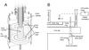Fig. 2 A) The Princeton MRI Experiment is a Taylor-Couette apparatus in which the end caps of the vessel have been divided in to two pairs of nested, independently rotatable end rings. B) The primary diagnostic of the fluid velocity is laser Doppler velocimetry (LDV). Radial profiles of vθ are acquired with the diagnostic viewing the fluid from the side. In the axial orientation two components of velocity vθ and vr are measured. Simultaneous measurement of the two velocities gives a direct measure of the r − θ component of the Reynolds stress. Due to very low data rates, the Reynolds stress is measured primarily at one point.

Zeldovich (1981) first applied Taylor’s torque measurements of cyclonic Couette flow to develop a closure model for Σ_rθ. Richard & Zahn (1999) extended Zeldovich’s analysis using the combined results of Wendt and Taylor to develop their closure model. We will focus here on the methodology of Richard and Zahn, but note that Longaretti (2002) arrived at a similar result using an eddy viscosity argument applied to the cyclonic data.

The closure model of Richard and Zahn proceeds from the scaling of the transition Reynolds number in the cyclonic data of Taylor and Wendt. The critical Reynolds number, Re_c, is a function of the gap between the cylinders Δr = r₂ − r₁. When the ratio of gap width to the average radius , , Re_c increases like . In this regime Richard and Zahn rewrite the critical Reynolds number in terms of the angular velocity gradient and arrive at an instability condition: $\mathit{R}{\mathit{e}}_{\mathrm{c}}\mathrm{=}\frac{\mathit{r̅}\mathrm{3}}{\mathit{\nu }}\frac{\mathrm{\Delta \Omega }}{\mathrm{\Delta }\mathit{r}}{\left(\frac{\mathrm{\Delta }\mathit{r}}{\mathit{r̅}}\right)}^{\mathrm{2}}\mathrm{\ge }\mathrm{6}\mathrm{\times }{\mathrm{10}}^{\mathrm{5}}{\left(\frac{\mathrm{\Delta }\mathit{r}}{\mathit{r̅}}\right)}^{\mathrm{2}}\mathrm{·}$(7)(We note that this prescription implies that the relevant length scale is rather than other length scales, Δr or h, an assumption which may not be justified. See Sect. 5 for more discussion.)

By this prescription, Richard (2001) should expect a turbulent transition at Re_c ≈ 7 × 10⁴ for the radius ratio . In the cyclonic experiments, a transition was observed at Re = 3 × 10⁴. However, the estimate for Re_c does not carry over to the anti-cyclonic experiment where a transition was observed at Re ≈ 3 × 10³. Also absent from the discussion leading to this equation is an estimate of the perturbation amplitudes which triggered the transitions in the experiments of Wendt and Taylor.

Torque measurements in the turbulent regime suggest to Richard and Zahn that the turbulent viscosity, ν_t, is a diffusive process and choose for it the form , α is a constant. Finally, using the observed approximate scaling of α with gap width, Richard & Zahn conclude that the local value for ν_t becomes independent of the gap width (for large enough gaps) and is determined only by the local shear: ${\mathit{\nu }}_{\mathit{t}}\mathrm{=}\mathit{\beta }\left|{\mathit{r}}^{\mathrm{3}}\frac{\mathit{\partial }\mathrm{\Omega }}{\mathit{\partial r}}\right|\mathrm{·}$(8)The flux of angular momentum is then given by $\mathit{\rho }{\mathit{r}}^{\mathrm{2}}\mathrm{⟨}{\mathit{v}}_{\mathit{r}}^{\mathrm{\prime }}{\mathit{v}}_{\mathit{\theta }}^{\mathrm{\prime }}\mathrm{⟩}\mathrm{=}\mathrm{-}\mathit{\rho }{\mathit{\nu }}_{\mathrm{t}}{\mathit{r}}^{\mathrm{3}}\frac{\mathit{\partial }\mathrm{\Omega }}{\mathit{\partial r}}\mathit{,}$(9)which can be rewritten in terms of q: $\mathit{\beta }\mathrm{=}\mathrm{-}\mathrm{⟨}{\mathit{v}}_{\mathit{r}}^{\mathrm{\prime }}{\mathit{v}}_{\mathit{\theta }}^{\mathrm{\prime }}\mathrm{⟩}\mathit{/}{\mathit{q}}^{\mathrm{2}}{\mathit{v}}_{\mathit{\theta }}^{\mathrm{2}}\mathit{.}$(10)Thus, β can be directly determined through measurements of the Reynolds stress. Finally, we comment on a particular case where ⟨v_θ⟩ satisfies the ideal Couette solution (Eq. (5)) with negligible ⟨v_r⟩ and axial dependences. In such a case, Eq. (6) reduces to $\frac{\mathrm{1}}{{\mathit{r}}^{\mathrm{2}}}\frac{\mathit{\partial }\mathrm{(}{\mathit{r}}^{\mathrm{2}}\mathrm{⟨}{\mathit{v}}_{\mathit{r}}^{\mathrm{\prime }}{\mathit{v}}_{\mathit{\theta }}^{\mathrm{\prime }}\mathrm{⟩}\mathrm{)}}{\mathit{\partial r}}\mathrm{=}\mathrm{0}$(11)where the specific angular momentum flux, ${\mathit{r}}^{\mathrm{2}}\mathrm{⟨}{\mathit{v}}_{\mathit{r}}^{\mathrm{\prime }}{\mathit{v}}_{\mathit{\theta }}^{\mathrm{\prime }}\mathrm{⟩}$ [=ν_tr³qΩ = β(r³qΩ)²], is a spatial constant. This is especially convenient when diagnostic access for Reynolds stress measurements are limited to certain locations. The Reynolds stress at other locations can be inferred.

3. Experiment

The Princeton MRI Experiment is a novel Taylor-Couette apparatus (Tagg 1994). The working fluid is confined between concentric, corotating cylinders which are bounded vertically by two pairs of nested, differentially rotating end rings (Burin et al. 2006; Schartman et al. 2009), Fig. 2. The experiment was designed to produce quasi-Keplerian flows of a liquid gallium alloy, GaInSn (Morley et al. 2008) which would become unstable to the MRI in the presence of an applied solenoidal magnetic field (Ji et al. 2001). To minimize the volume of GaInSn required for the MRI studies, the height of the cylinders is only twice the gap width between them, $\mathit{h}\mathit{/}\mathrm{\Delta }\mathit{r}\mathrm{=}\mathit{h}\mathit{/}{}^{\mathrm{(}}\mathit{r}_{\mathrm{2}}\mathrm{-}{\mathit{r}}_{\mathrm{1}}{}^{\mathrm{)}}\mathrm{\approx }\mathrm{2}$. This aspect ratio is small in comparison with other Taylor-Couette experiments which aim to minimize the influence of the end caps by separating them as much as possible. For example, Taylor (1936) used h/Δr > 100. Further details of the design and implementation of the apparatus and diagnostics can be found in Schartman et al. (2009).

3.1. Apparatus

The experiment outer cylinder is a pressure vessel into which the inner cylinder and end rings are submerged. The outer cylinder is a 25.4 mm thick annulus of cast acrylic capped by two 101.6 mm thick acrylic disks. The inner cylinder and end rings are mounted to nested stainless steel axles which pass through the top cap of the outer cylinder. The rings are acrylic. The lower rings and outer cylinder cap were polished to allow optical diagnostic access to the fluid. The inner cylinder is stainless steel and was painted black to reduce reflections which would interfere with the velocity measurement (Table 1). A lip seal is mounted at the top end of each axle to seal against its inner neighbor. The submerged, lower, end of each component is fixed radially by a plain bearing.

The hydrodynamic experiments reported here use water or a water-glycerol mix as the working fluid. The kinematic viscosity of the water-glycerol mix is ν_mix = (15 ± 1)ν_water, with a density of 1.2 g/cm³.

The Princeton MRI Experiment also differs from previous Taylor-Couette experiments in the low tolerance of several components. The submerged plain bearings have radial “play” ranging up to 0.1 mm. Because those bearings are nested, they contribute to a total run-out of the inner cylinder of up to 0.8 mm, see Schartman et al. (2009).

3.2. Experimental flow profiles

The component speeds used to develop the azimuthal velocity profiles are enumerated in Table 2. The four component speeds are listed as ratios to the outer cylinder rotation speed. Our flows of primary interest are the two quasi-Keplerian profiles with nominal values based on the cylinder speeds of q = 1.5 and 1.9. The flow shear of the former is most analogous to accretion flow and for convenience we refer to it as “QK(q = 1.5)”. The fastest growing mode of the MRI has a growth rate  | ω_max | ∝ | qΩ | , therefore the value of q = 1.9 was selected to take advantage of this. The q = 1.9 flow is divided into the three named profiles “QK(Ekman)”, “QK(Split)” and “QK(q = 1.9)” to reflect the choice of end ring speeds. “Ekman” refers to the boundary layer that we expected to significantly perturb the ideal profile, as was seen in a prototype experiment with h/(r₂ − r₁) = 1 (Kageyama et al. 2004). “Split” duplicates the end cap condition commonly used in Taylor-Couette experiments, such as with Taylor, Richard and Wendt (though Wendt had no upper cap, but a free surface). In the “QK(q = 1.9)” profile the end rings are rotating at speeds intermediate to those of the cylinders. The particular choice of speeds were arrived at by trial and error to best approximate the ideal Couette profile, Eq. (5). Radial profiles of v_θ for the q = 1.9 profiles will be presented in Sect. 4.3.

In addition to the quasi-Keplerian profiles, we also present measurements of Σ_rθ from three other anti-cyclonic flows: MS, CUS 1 and CUS 2. They were chosen to lie at or above the Rayleigh centrifugal stability limit. MS refers to a configuration for which the end ring and inner cylinder speeds have been scaled up to the marginal stability line, q = 2. For the cylinder radii we have chosen, the Rayleigh criterion is reached when the inner cylinder speed is ${\mathrm{\Omega }}_{\mathrm{1}}\mathrm{=}{\mathrm{\Omega }}_{\mathrm{2}}{\mathit{r}}_{\mathrm{2}}^{\mathrm{2}}\mathit{/}{\mathit{r}}_{\mathrm{1}}^{\mathrm{2}}\mathrm{=}\mathrm{8.27}$, the CUS profiles are centrifugally unstable by this criterion. For CUS 1, the speed of the inner cylinder and the end rings have been scaled by a constant from those of the QK(q = 1.9) configuration by 15% above the Rayleigh criterion. To make the flow even more unstable, the CUS 2 profile has had the outer end ring and outer cylinder speeds set to zero. Radial profiles of for the CUS cases were not measured. Measurements of transport in the turbulent centrifugally unstable cases are reported in Burin et al. (2010).

The flow profiles are established through an impulsive acceleration of the rotating components. Most often, the experiment was started from rest, though a transition from solid body to differential rotation was also common. The abrupt change in boundary speeds causes the fluid to spin up via Ekman pumping rather than viscous diffusion, though shear instabilities at the walls may contribute to spin-up at early times. The Ekman timescale governs the equilibration time, τ_E ~ (L²/νΩ₂)^1/2. When Ω₂ = 5.6 rad/s, τ_E ~ 60 s. We observed that the fluctuation levels reached their equilibrium values after approximately five viscous Ekman times, and so waited a minimum of 300 s before performing flow measurements (Schartman et al. 2009).

3.3. Diagnostics

3.3.1. Laser Doppler velocimetry

We use LDV for two types of measurement depending on the orientation of the diagnostic with respect to the apparatus, see Fig. 2. When the diagnostic is oriented to view the fluid through the outer cylinder wall, radial profiles of azimuthal velocity, v_θ, are acquired. Viewing the fluid from beneath the vessel, we measure simultaneously v_θ and v_r with a correlation window of 10 μs between them. Thus, all fluctuations are measured up to the frequency of 10⁵ Hz, which is comparable to the Doppler frequency of structures at the viscous scale in water or the size of the tracer particles used. All flows are calibrated against solid body rotation.

In this experiment, the primary sources of error in the LDV measurement are due to optical properties of the acrylic outer cylinder. The errors arise from the curvature of the cylinder, misalignment of the probe head with respect to the vessel and random defects in the optical path. The random defects arise through stress-induced variations in the refractive index of the acrylic. The variations most likely induce spurious correlations by altering the focal lengths of the LDV beams (Miles 1996). The velocity measurement is proportional to sin(d/2f), where d is the beam separation and f is the focal length. Varying the focus for both v_r and v_φ measurements simultaneously will introduce a simultaneous over or underestimation of the velocities. The mean error is removed by calibration against solid body rotation. However, the random defects broaden the sample distribution of the velocity measurement, which cannot be eliminated. The limiting precision of LDV is v′/v ≈ 0.1%, whereas our precision was 1.5%. Details of the calibration process can be found in Schartman (2008).

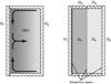Fig. 3 End cap effects which were predicted to distort significantly the mean profile of vθ from the ideal Couette solution. Left: in the bulk flow the velocity profile is supported by the radial pressure gradient, ${\mathit{v}}_{\mathit{\theta }}^{\mathrm{2}}\mathrm{\left(}\mathit{r}\mathrm{\right)}\mathit{/}\mathit{r}\mathrm{=}\mathit{\partial p}\mathit{/}\mathit{\partial r}$. The pressure is approximately uniform vertically, but at the end caps the non-slip boundary condition requires vθ = rΩ2. This imbalance at the end cap drives the radial Ekman circulation, when Ω2 < Ω1 the flow is directed inward. When the Ekman flow reaches the inner cylinder it transitions to an axial flow. In a small aspect-ratio device such as the Princeton MRI Experiment (Kageyama et al. 2004) predict that the Ekman circulations would meet at the midplane and form a radial jet. Right: with independent end rings, the strength of the Ekman pumping can be reduced by minimizing the velocity difference between the rings and the bulk flow. The simulations of Kageyama et al. (2004) showed that two rings provided an effective trade off between mechanical complexity and reduced Ekman pumping. A simulation of the two-ring design by Hollerbach & Fournier (2004) predicted the formation of Stewartson layers at the boundaries between the components. The ideal Couette profile would then be replaced by two annuli in solid body rotation with the end rings.

When the LDV was setup to measure radial profiles of v_θ, the beam probe head is oriented to view the fluid through the curved outer cylinder wall. The laser paths for the velocity component tangent to the azimuthal angle enter and exit the cylinder wall at non-normal incidence. As the probe is scanned radially the angles of incidence change, which alters both the radial location and magnitude of the v_θ measurement, see Schartman (2008). The location of the axial velocity measurement did not coincide with that of v_θ so Σ_θz could not be measured. Moreover, the v_z measurement location was often outside of the flow volume, so this velocity component was ignored.

When the LDV diagnostic is oriented axially to measure v_θ and v_r, the beam path passes through the cylinder bottom cap and outer ring. Attenuation of the laser intensity due to the four boundary crossings limits the data rate to order 1 Hz. For the previously reported measurements of the radial-azimuthal component of Reynolds stress (Ji et al. 2006; Burin et al. 2010), we required of order 10³ velocity samples per fluid profile. Because of this time demand, LDV was performed at only one radial location in this orientation. The LDV probe head was oriented such that the beam bisector was approximately normal to the acrylic surfaces. Comparison with the expected velocity value for solidbody rotation revealed an offset of about 3% in the magnitude of the v_θ.

3.3.2. Flow visualization

Flow visualization of CU, QK(Ekman) and QK(q = 1.9) profiles was performed using water with a 0.3% addition of Kalliroscope AQ-1000 rheoscopic concentrate. The Kalliroscope flakes align with the local fluid shear. The intensity and direction of light scattered by the flakes to make flow patterns visible (Savas 1985). In laminar circular Couette flow the surface normal of the flakes align parallel to . Illuminated from below, ideal (and stable) Couette flow should appear as a uniform color. The flow over the outer ring was illuminated from below by a flashlight and imaged from the side by a CCD.

An attempt to image the flow over the inner ring using this method was not successful. The broad area of illumination combined with the low Kalliroscope concentration required to view the inner region of the flow could not produce enough contrast in the CCD to generate useful images.

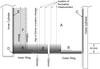Fig. 4 Regions of flow within cylinder gap MRI operation, in this case the outer ring is rotating slower than the bulk flow and the inner ring corotates with the bulk flow at r = 120 mm. The lower half of the apparatus is shown. A) The Taylor-Proudman theorem holds in the bulk flow, which closely approximates the ideal Couette profile. B) Fluctuations generated by the vertical boundaries extend approximately 40 mm into the flow. The sign of radial circulation within the “boundary zones” are indicated by the horizontal arrows. At r = 120 mm, the boundary corotates with the bulk flow. The radial velocity of the Ekman circulation changes sign at this radius as the ring is removing (adding) angular momentum to the bulk at smaller (larger) radii. The Ekman circulations penetrate into the bulk flow, see Fig. 8. Near the ring gap a vertical scan of vθ fluctuations indicates that the discontinuity in velocity produced at the ring gap does not propagate in to the bulk flow. C) Centrifugally stable boundary which transitions from the bulk flow to the outer cylinder. (This region C may be centrifugally unstable when the cylinder speeds exceeds the Rayleigh criterion as in the flow CUS 1 listed in Table 2. This leads to a lower q than 2 in the region A), and may explain the small measured Reynolds stress there as shown in Fig. 10). D) Ekman layer detaches from walls with higher fluctuations visible in the 5 mm radial scan, see Fig. 7. The maximum fluctuation amplitude due to the detachment is approximately 37% and occurs at r ≈ 105 mm (Schartman 2008). E) Measurement of q indicates a centrifugally-unstable region exists between the inner cylinder and r1 ≈ 90 mm. F) The unstable flow relaminarizes by r = 100 mm.

3.4. End caps effects: Ekman and Stewartson layers

All physically realizable Taylor-Couette experiments have a finite cylinder height, h. Rigid plates form the vertical boundaries, with some exceptions such as Wendt (1933) who used a free upper fluid surface. The non-slip boundary conditions at the end caps may introduce deviations from the ideal Couette profile, Eq. (5). The influence of the boundaries is never completely negligible even for aspect ratios in excess of 100 (Taylor 1936; Tagg 1994). Two possible effects of the boundaries are to produce Ekman (Greenspan 1968) or Stewartson layers (Stewartson 1957).

In the bulk flow pressure balances the centrifugal force of the velocity profile, 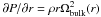$\mathit{\partial P}\mathit{/}\mathit{\partial r}\mathrm{=}\mathit{\rho r}{\mathrm{\Omega }}_{\mathrm{bulk}}^{\mathrm{2}}\mathrm{\left(}\mathit{r}\mathrm{\right)}$. The pressure is approximately constant vertically, while the velocity in the viscous layer attached to an end cap is rotating at the end cap speed, Ω_cap. At the interface between the bulk flow and the viscous layer, a radial Ekman flow is generated to balance the discontinuity of force, see Fig. 3. If Ω_cap < Ω_bulk, the Ekman flow is directed inward radially. When the layer reaches the inner cylinder, it transitions to an axial flow and is accelerated as it spirals along the cylinder. In large aspect ratio devices, the Ekman layer may detach from the inner cylinder before reaching the midplane (Coles 1965). In small aspect ratio devices such as our prototype (Kageyama et al. 2004) we observed that the Ekman layers from each end cap propagated to the cylinder midplane. The flows at the juncture then detached from the inner cylinder in a radial jet. The advection of angular momentum by the Ekman layers produced a mean radial profile of v_θ which was centrifugally unstable near the inner cylinder, and flattened over the larger radii. The cylinders of the current apparatus are only a factor of two taller than the prototype, so we expected a similar effect occur when both end rings co-rotate with the outer cylinder.

Stewartson layers arise from the tendency of a rotating flow to be uniform along the axis of rotation, at least on timescales long compared to an Ekman time, τ_E. Simulations by Hollerbach & Fournier (2004) of the Princeton MRI Experiment predicted the formation of Stewartson layers at the boundaries of the end rings, see Fig. 3. The layers are predicted to separate the bulk fluid in to two annuli. The inner annulus would be in solid body rotation with the inner end rings, and the outer annulus with the outer end rings. The narrow shear layers between the two annuli, and between the annuli and cylinders would be unstable (Hide & Titman 1967; Früh & Read 1999).

Two experiments using LDV were performed to determine the extent to which Ekman or Stewartson layers cause the bulk flow to deviate from the ideal Couette profile. The first experiment was to compare the radial profiles of v_θ using end ring speeds which would maximize or minimize the strength of the Ekman circulation. The second experiment was a detailed vertical scan of v_θ near the ring gap for the profile which minimizes the Ekman circulation. The results of these experiments are presented in Sect. 4.3.

4. Results

4.1. Topography of the QK(q = 1.9) profile

Before presenting the details of the experiments, the topography of a flow generated in the QK(q = 1.9) configuration is diagrammed in Fig. 4. The QK(q = 1.9) profile is displayed because it demonstrates the greatest diversity of behavior in the apparatus. The profiles generated by a different choice of end ring speeds feature one or more of the behaviors of the QK(q = 1.9) profile. The profile consists of a bulk flow in which the Taylor-Proudman theorem holds, and is bounded at the cylinder walls by thin shear layers. The layer at the inner cylinder is anti-cyclonic and unstable by Rayleigh’s criterion. The layer at the outer cylinder is cyclonic, and therefore stable. Ekman layers are present on the top and bottom end rings. One radius of the inner ring corotates with the bulk flow. On either side of this radius the Ekman flows change sign and the flows are able to penetrate deeply into the bulk flow. No radius of the outer ring corotates with the bulk flow, confluence of Ekman circulation does not occur.

The Kalliroscope images of Fig. 5C indicate the most obvious characteristic of the flow: a bulk profile in which the Taylor-Proudman theorem holds, is bounded above and below by a turbulent layer. The measurement of Σ_rθ which extended from z = 35 mm up to z = 90 mm shows no evidence of turbulent radial transport. Mechanical limits of the LDV diagnostic prevented measurements closer than 35 mm to the boundary. From Fig. 7 the region in which the Taylor-Proudman theorem holds extends to at least 5 mm from the end rings. We also know from Fig. 8 that the fluctuation levels of v_θ are increasing as the end ring is approached. Both of these imply the existence of a vertical Reynolds stress Σ_θz. Our ability to place a bound on Σ_θz is limited by the uncertainty in the magnitude of $\overline{{\mathit{v}}_{\mathit{r}}}\mathrm{=}\mathrm{0.18}\mathrm{\pm }\mathrm{0.17}$ mm/s (Schartman 2008).

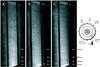Fig. 5 Kalliroscope image of three flows at Re ≈ 5 × 105. A) centrifugally unstable flow with  [Ω1,Ω3,Ω4,Ω1] = [41.8,0,0,0]  rad/s. B) A quasi-Keplerian flow using the Ekman configuration, QK(Ekman),  [Ω1,Ω3,Ω4,Ω1] =   [41.8,5.6,5.6,5.6]  rad/s. C) A quasi-Keplerian profile with end ring speeds optimized to produce the best approximation to the ideal Couette flow 5, QK(q = 1.9),  [Ω1,Ω3,Ω4, Ω1] = [41.8,15.3,4.2,5.6]  rad/s.

4.2. Flow visualization

Images taken with the Kalliroscope technique are shown in Fig. 5. The three flows shown are a CUS 2 centrifugally unstable flow with the outer cylinder at rest, QK(Ekman) flow with the end rings co-rotating with the outer cylinder, and a QK(q = 1.9) profile with both rings in differential rotation. The Reynolds numbers of the profiles are all approximately 5 × 10⁵.

In the centrifugally unstable case, the turbulence is fully developed. There are no visible large scale flow patterns. As discussed in Burin et al. (2010) this lack of structure is consistent with other experiments of supercritical flow at large Reynolds numbers (Lewis & Swinney 1999). The QK(Ekman) case has less structure than the QK(q = 1.9) flow, though we will show in Sect. 4.4 that a larger Reynolds stress is present in the QK(Ekman) flow. In the QK(q = 1.9) case the flow appears turbulent within about 40 mm of the end ring boundary, but in the bulk of the flow the uniform horizontal streaks indicate a quiescent flow. Note also that only in the QK(q = 1.9) case does enough light reach the top ring to discern the upper turbulent band. This demonstrates that the flakes are most aligned with the rotation axis, consistent with the hypothesis that the velocity shear is radial.

4.3. Radial profiles of quasi-Keplerian flows

A comparison of three quasi-Keplerian flows is plotted in Fig. 6. The speeds of the inner and outer cylinders are 42.0 and 5.6 rad/s, respectively. The Reynolds number is Re = 5.5 × 10⁵ and the nominal value for 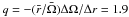. The end rings rotate in the QK(Split), QK(Ekman), or QK(q = 1.9) configurations.

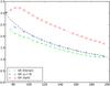Fig. 6 ⟨vθ⟩ for three different centrifugally stable profiles at Re = 5 × 105. The dashed line is the ideal Couette profile based on the cylinder speeds, Ω1 = 42.0,Ω2 = 5.6 rad/s. The dotted lines are cubic spline fits to the bulk flow. The innermost velocity measurement overlaps the inner cylinder and is therefore not included in the interpolation. Both the systematic and random errors in ⟨vθ⟩ are smaller than the marker size.

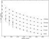Fig. 7 Radial profiles of vθ at several axial locations for an optimized flow (QK(q = 1.9)) at Re ≈ 3 × 105. To facilitate viewing the profiles have been offset. The increased fluctuation levels in the 5 mm scan near the inner cylinder are due to the disruption of the boundary layer circulation which occurs for differential rotation of the inner cylinder with respect to the inner ring. For the innermost radial point at 72 mm, the measurement volume of the diagnostic overlaps the inner cylinder and is therefore a measure of the surface speed of the cylinder rather than a flow velocity.

Radial profiles of V_θ at several axial heights are plotted in Fig. 7 for the QK(q = 1.9) configuration. The axial positions vary from 5 mm above the lower rings to the midplane at 140 mm. The plotted profile is at Re = 3 × 10⁵ with Ω₁ = 21.0,Ω₃ = 7.6,Ω₄ = 2.1,Ω₁ = 2.7 rad/s. The thickness of the viscous Ekman layer is 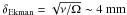${\mathit{\delta }}_{\mathrm{Ekman}}\mathrm{=}\sqrt{\mathit{\nu }\mathit{/}\mathrm{\Omega }}\mathrm{~}\mathrm{4} \mathrm{mm}$. The profiles indicate that the Taylor-Proudman theorem holds in the bulk of the flow, but does not all the way to the end rings. This is especially true for the outer ring which is rotating slower than the outer cylinder. The deviation from the mean profile near the inner cylinder in the 5 mm data is due to an intermittent presence of the boundary layer as it is ejected from the inner cylinder-inner ring transition, see Schartman (2008). The plotted profile is stable by the Rayleigh criterion but two vertical shear layers are present at the cylinder walls.

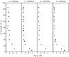Fig. 8 Azimuthal velocity fluctuation levels, σvθ/⟨vθ⟩, near the ring gap for the QK(q = 1.9) profile at Re = 5 × 105 shown in Fig. 7. The radial locations of the scans are diagrammed in Fig. 4. Triangles are the QK(q = 1.9) profile. Shown for comparison are the solid body levels, dotted lines and one axial location for a QK(Ekman) profile, squares. Note that in the r = 123 mm panel, the solidbody line nearly overlaps the left plot border.

A detailed vertical scan was performed near the ring gap to look for evidence of the Stewartson layer predicted by Hollerbach & Fournier (2004). The results of that scan are plotted in Fig. 8. The scan was performed at four radii: r = 123, 129, 134 and 140 mm which are shown in Fig. 4 as the vertical dashed lines. For the radii 129, 134 and 140 mm the fluctuations levels, σ_vθ/⟨v_θ⟩, are comparable to the solid body fluctuation amplitude which is plotted as the vertical dotted lines. No evidence of a Stewartson layer is present near the ring gap at 132 mm. For the points at r =123 mm, the fluctuation amplitude does not converge to the solid body value but remains slightly elevated through to the experiment midplane. The reason for this is that a Stewartson layer does form in the vicinity of the radius at which the end ring co-rotates with the bulk profile, Ω₃ = Ω(r = 123 mm). A single radial scan using a QK(Ekman) profile is also plotted, marked by the squares. In the QK(Ekman) configuration the end caps rotate with the outer cylinder and because of the absence of a stationary radius in the bulk flow, the fluctuation level is comparable to the sold body level. The fluctuation levels of the Stewartson layer at 123 mm are comparable to fluctuation levels over the outer ring in CUS flows in which the outer cylinder is rotating (Schartman 2008).

To perform the measurement of β given in Eq. (10) we need the Σ_rθ component of the Reynolds stress and a value for the local exponent of angular velocity, q. Correlated two-component LDV provides the measurement of Σ_rθ. We determine q from the radial profiles of v_θ plotted in Fig. 6. Because of the proximity of the radial boundaries it is tempting to compute an average value based on the cylinder speeds: . Using this formulation, the three profiles in the figure have the same value for q. A cursory inspection shows that the QK(Split), QK(Ekman) and QK(q = 1.5) profiles do not share the same gradient at r = 180 mm.

Instead we compute q based on a cubic-spline interpolation of v_θ. Determination of q was also done using a finite difference scheme, see Schartman (2008) with similar results. The interpolation of the profile is plotted as the dotted lines in Fig. 6. Radial profiles of q for the QK(Split), QK(Ekman) and QK(q = 1.9) configurations are plotted in Fig. 9. We note that the q value for the QK(q = 1.9) configuration is actually larger than 2 near the outer cylinder but without apparent local centrifugal instabilities.

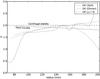Fig. 9 q profiles for centrifugally stable flows used in the calculation of β. The profiles are calculated using the spline fit presented in Fig. 6. Schartman (2008) used a finite difference method to evaluate q producing comparable results. q profiles are also plotted for ideal Couette fow, and marginal stability by the Rayleigh criterion q = 2. The stability boundary derived by Rayleigh (1916) and Taylor (1923) do not account for the presence of vertical boundaries. The oscillation in the QK(Split) case which occurs between 140 and 180 mm is due to the measurement of vθ beginning before the flow had fully equilibrated.

4.4. Reynolds stress

Errors in the measurement of β are dominated by random and systematic errors in ⟨v_rv_θ⟩. We reduced the random error by acquiring of order 10³ samples for each measurement. The systematic error is removed by subtracting the correlation level measured in a solid body profile. The sources of the systematic error include any defects in the acrylic vessel and rings along the laser optical path and any residual inherent correlations between the two components of LDV systems as discussed in Sect. 3.3.1. Example data and their comparisons can be found in Fig. 3 from Ji et al. (2006). The transport levels for linearly-stable profiles are plotted in Fig. 10. The measurements are performed at r = 179 mm and z = 62 mm or z = 74 mm, but the results are robust for other locations, see Fig. 3 from Ji et al. (2006) for the z-dependence. The optimized QK(q = 1.9) and QK(q = 1.5) configurations for Re > 10⁶ are not consistent with Richard and Zahn’s proposed transport level. Averaging the results for the optimized configurations yields β = (1.13 ± 1.15) × 10^-6 and β < 3.4 × 10^-6 at 2 standard deviations. Because negative values for β would indicate inward transport of angular momentum (which we believe to be unphysical, as it would intensify rather than extract energy from the shear), 2 standard deviations yields 98% confidence. The slight improvement of the transport limit over the previously published result (Ji et al. 2006) is due to the use of the local measurement of q and a correction for a small angular misalignment of the LDV diagnostic.

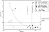Fig. 10 Measurement of β for quasi-Keplerian profiles at r = 179 mm and z = 62 mm or 74 mm. Horizontal dashed lines is the predicted range of β from Richard and Zahn. The vertical dashed line is the estimate of the transition Reynolds number predicted by Eq. (7).

Choices of the ring speeds other than the optimized values have profound effects, through the global Ekman circulation, on the mean flow profiles (Fig. 6) as well as on the Reynolds stress, Σ_rθ. When the ring speeds are chosen to be equal to the outer cylinder (the QK(Ekman) configuration), Σ_rθ is raised significantly above the zero line as shown in Fig. 10, even above the Σ_rθ value measured in the CUS 1 configuration which has a local q below 2 in the bulk flow but with a centrifugally unstable layer near the outer cylinder (the region C in Fig. 4). We note that the Σ_rθ value in the QK(Ekman) configuration approaches the level proposed by Richard & Zahn (1999). When the inner (outer) ring rotates at the inner (outer) cylinder speed (the QK(Split) configuration), Σ_rθ jumps to much larger values. It is important to note that the QK(Split) configuration has stability only with respect to the two cylinder speeds but is unstable locally, i.e. at the ring gap. Given this level of transport, the observations by Richard (2001), which uses the split configuration, are likely to be caused by the influence of the end rings extending throughout the fluid volume. As a side note, the axial boundary conditions are also important for cyclonic flows briefly studied in the Princeton MRI experiments. In the split configuration, radial profiles of these cyclonic flows deviated significantly from the ideal Couette profiles with large fluctuations (Burin 2006), and this subject is studied in detail by a followup experiment (Burin & Czarnocki 2012).

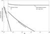Fig. 11 A simplified Moody diagram for circular pipe flow. Only three transport curves are shown: the laminar case, turbulence in a pipe with smooth walls, and one choice of rough wall turbulence. For the rough wall curve, the scale height of the roughness is 5% of the pipe diameter. Below the minimum critical Reynolds number, a perturbed flow will always return to the laminar state. A transition to the turbulent state is marked by a discontinuity in the transport level. The minimum magnitude of the discontinuity in this case is approximately 2.

If a subcritical transition occurred in the range 3 × 10⁵ < Re < 2 × 10⁶, what should we expect to see in Σ_rθ? Suppose the transport follows the behavior of the normalized pressure drop, or friction factor, plotted in the Moody diagram of pipe flow (Moody 1944). A simplified moody diagram is reproduced in Fig. 11 which displays only the laminar behavior and two turbulent cases. The turbulent curves are the smooth wall case and one rough wall case in which the scale height of the roughness is 5% of the pipe diameter. A jump should occur at the transition from the laminar value to a value of order a few times the laminar transport level. If the flow is bounded by rough walls the friction factor should approach constant or logarithmic behavior when the viscous boundary layer becomes thinner than the roughness scale height. This formed the basis of our astrophysical extrapolation in Ji et al. (2006). However, our end caps are not rough nor is rough-wall behavior applicable to accretion disks. Instead, once the transition occurs the transport should again be a decreasing function of Reynolds number. If a transition occurred in the proposed range we should see, according to the Moody diagram, Σ_rθ jump to a factor of 2 to 4 above the laminar transport level β_visc (where shown in Fig. 10) and then fall off as Re is further increased. The absence of such a spike in Fig. 10 argues strongly against the presence of a transition.

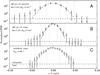Fig. 12 Probability densities of vr for QK(q = 1.9) configuration at Re ≈ 2.2 × 104 using water-glycerol mixture (top panel, labelled A in Fig. 10), QK(q = 1.9) configuration at Re ≈ 3.3 × 105 using water (middle panel, labelled B in Fig. 10), and solid-body rotation (bottom). Apparently larger standard deviations in the solid body flow (C) than those in the QK flow in water (B) are due to the larger ΩOC in the flow (C). The curves are Gaussian fits to the data, vertical lines are first, second and third standard deviations from their means . The data were acquired at z = 75 mm. Note that non-Guassian tails at the level of ≈ 0.2 are due to acrylic optical defects and not genuine characteristics of the flows.

The source of the higher levels of transport associated with the glycerol runs are hinted at by the time-averaged radial velocities (Schartman 2008). Of the QK(q = 1.9) configurations, only for these low Reynolds number experiments is statistically distinguishable from zero. For example, at Re = 2.2 × 10⁴ with glycerol  mm/s, whereas for water  mm/s at Re = 3.3 × 10⁵. The v_r distributions for a glycerol run are compared to a water run and a solid body water run in Fig. 12. At Re = 2.2 × 10⁴, fluctuations are clearly present in the negative tail of the distribution which give rise to the non-zero value of . At the same speed but in water (so that Re = 3.3 × 10⁵), the fluctuations are more symmetric about the mean and the mean radial velocity has fallen by a factor of two. We interpret this to mean that the residual unsteady secondary circulation penetrates deeper into the bulk flow at lower Re, consistent with the results from numerical study by Obabko et al. (2008) which was performed at relatively low Re.

5. Discussions and conclusions

When operating in the QK(q = 1.9) and QK(q = 1.5) configurations with minimized Ekman effects we find no evidence of significantly enhanced angular momentum transport due to the r − θ component of the stress tensor, even at Re ~ 10⁶. The absence of the measured transport efficiencies significantly above their laminar counterparts provides no evidence for a turbulent transition in our quasi-Keplerian flows in the range 10⁴ < Re < 10⁶ since turbulence should enhance the transport to release the free energy it results from. If a subcritical transition occurs at a greater Reynolds number, experiments with Poiseuille flow indicate that at the transition the amplitude of the dimensionless turbulent transport will be a factor of a few above the laminar viscous value which decreases as Re^-1. The tendency of the normalized turbulent intensity to vary inversely with the critical Reynolds number has been confirmed for cyclonic flows, and also for anticyclonic flows to a lesser extent, by the numerical simulations by Lesur & Longaretti (2005). We therefore conclude that either a subcritical transition does not occur, or, if a subcritical transition does occur, the associated radial transport of angular momentum is too small to directly support the hypothesis that subcritical hydrodynamic turbulence is responsible for accretion in astrophysical disks.

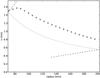Fig. 13 Split end-cap operation at Re = 3 × 105. The dotted line is the ideal Couette profile. The dashed lines are the solid-body speeds of the end rings. Based on the cylinder speeds, the flow should be stable by the Rayleigh criterion. Our beta measurement indicates that the bulk flow is in a turbulent state. Only Rayleigh-unstable flows with the outer cylinder at rest were observed to have greater levels of transport.

This picture conflicts with the observations of Richard (2001) in which flow imaging demonstrated a turbulent transition in quasi-Keplerian flow near Re ~ 10⁴. Richard attributes the turbulence to SHI, but alternative hypotheses were not ruled out. In particular, our measurements in Split end-cap operation indicate that a detached shear layer is present above the inner ring. Such layers are known to have a non-axisymmetric linear instability (Hollerbach 2003; Schaeffer & Cardin 2005). A plot of QK(Split) configuration at Re = 3 × 10⁵ is reproduced in Fig. 13. Also plotted are the velocities of the end rings, as dashed lines. A centrifugally unstable layer is present near the outer cylinder therefore the flow in the vicinity of 200 mm is strongly turbulent. This observation is confirmed by Σ_rθ measurement for this flow: only in the CUS 2 case was a greater level of turbulent transport observed. The inflection point at r ≈ 85 mm has relaxed significantly from the solid body line of the ring which indicates that this region is the source of the instability. The precise nature of the instability cannot be inferred from this saturated flow. As noted, an inflection point is linearly unstable. But it is also possible that flow undergoes an axisymmetric transition because the fluid in solidbody rotation with the end ring has effectively increased the inner cylinder radius.

There are possible limitations in applying the our results directly to astrophysical disks due to experimental geometry. Typical cold and dense astrophysical disks, such as protostellar disks, are geometrically thin, following the ordering , which contrasts with the scale ordering for our experimental apparatus, where all three scales are similar, a point that was made by one of our referees (Longaretti) as well as by Mukhopadhyay & Saha (2011). We now discuss the role of experimental geometry on our conclusions, namely with respect to aspect ratio (h/Δr) and normalized curvature ().

The dependence of the subcritical transition and turbulent transport on aspect ratio (h/Δr) is essentially unknown due to the absence of a first-principles theory. However, conceptually, in the absence of vertical friction, the vertical scale h should not play a role in the transition Re or in radial turbulent transport due to the instability’s origin in radial shear at least when h is larger than both r and Δr, as it is in our experiment. In disks, h (scale height of disk, or some fraction thereof due to stratification) may play more of a role in limiting the size of the largest eddies (or other structures) in the r − z plane (Dubrulle et al. 2005). How this limitation would ultimately affect angular momentum transport is unknown, though a reduction in transport may be implied.

In experiments, the ratio h/Δr may serve as a proxy for the strength of secondary flows due to viscous boundaries. These secondary flows may perturb the flow and trigger instability in subcritical flows – Richard (2001) and Paoletti & Lathrop (2011) (see below) probably being examples of this. These boundary-driven flows contribute to the radial momentum transport. Examples to the contrary, where secondary flows suppress instability and transport, are not known in high-Re Taylor-Couette flow. Our end-cap controls, when optimized, have allowed us to reach relatively high Re while maintaining a quiescent state. Non-optimized end-cap conditions (similar to those used by other expreriments with less controllable boundary conditions), on the other hand, produce fluctuations due to finite h. Thus our optimized velocity measurements, both mean and fluctuating, are suggestive of ideal flow.

Even if h is insignificant, the role of curvature is not, and it remains uncertain as to which radial length scale is relevant. Richard & Zahn (1999) showed that the relevant length scale in the cyclonic flows (based on Wendt 1933; Taylor 1936) changed from Δr to for . An inferred quadratic scaling above this boundary yields Re_c ~ 6 × 10⁵ for the parameters of our experiment, a value which we have exceeded. Thus, even taking into account the effects of flow curvature, the lack of the evidence of turbulence in our results is significant. It is unclear though to what extent scalings based on cyclonic data may be applied to the anti-cyclonic quasi-Keplerian regime.

Recent experimental work by Burin & Czarnocki (2012) in cyclonic flows illustrates that in experiments with large Δr, only a fraction of the flow becomes turbulent, a fraction that reflects the fact that the shear gradient in these experiments is localized near one of the cylinders. Outside of this region the flow remains laminar even well past Re_c. Thus the scaling of Richard & Zahn (1999) appears to be an overestimate. In any case, this is not relevant to disks, where the balance between gravitational and centrifugal forces enforces a nearly constant ratio of shear to rotation.

One might ask a subtle but relevant question, as raised by an anonymous referee, on whether our chosen axial boundary conditions for the ideal Couette profile might limit the transition or turbulent transport from occurring in the bulk flow. This question is motivated by the fact that some well-known subcritical transitions in non-rotating flows are accompanied by large changes in the mean flow; see a recent study in a plane Couette flow by Krug et al. (2012). While it is not possible to completely rule out such a possibility since the transition mechanism is not understood, but it seems unlikely. The axial boundaries can influence the bulk flow either through global Ekman circulation or through local vertical vortex tubes in the spirit of Taylor-Proudman theorem. The former process is slow on a timescale  ∝ Re ^− 1/2 as shown previously (Kageyama et al. 2004), and it is unlikely to be dynamically important for the transition in the bulk flow. The latter process requires more rapid global rotation (Spence et al. 2012) or a strong axial magnetic field in an electrically conducting fluid (Roach et al. 2012); none of them applies here. In fact, the enhanced fluctuations observed near the axial boundaries (Figs. 5C and 8) are indicative of the existence of a turbulent boundary where Taylor-Proundman theorem should not apply.

As a final note, we briefly remark on a new paper (Paoletti & Lathrop 2011) that we were informed just before our planned submission of the present paper. The authors presented a β value of (1.7 ± 0.2) × 10^-5 inferred from torque measurements in quasi-Keplerian flows at similar Reynolds numbers to ours. Since this β value is significantly above ours from direct measurements of Reynolds stress, it was claimed that a turbulent state is seen. We point out, however, that the large β values measured there are subject to the interpretation based on the Ekman effects caused by axial end caps corotating with the outer cylinder. In fact, their reported β value is only by a factor of 2 larger than that of our QK(Ekman) flow (see Fig. 10), which has a reduced Ekman circulation due to a disrupted boundary layer despite the small aspect ratio (Schartman et al. 2009). Richard (2001) reported significant Ekman effects in quasi-Keplerian flows with corotating end caps (and also in the Split configuration) as indicated by large deviations of the measured velocity profiles from the ideal Couette solution (see his Fig. 4.2). Velocity profiles are unreported in Paoletti & Lathrop (2011) but their aspect ratio of 11.47 is smaller than  ~ 25 in Richard (2001), and thus should be subject to stronger Ekman circulations. This latter point is consistent with recent results from numerical simulations (Avila 2012) which were performed at Re significantly below experimental values. The reported numerical results also showed turbulence in the bulk flow in our experimental geometry at low Re. However, these results do not necessarily contradict our data reported in the present paper: the measured β values (e.g. the point A in Fig. 10) are significantly larger at lower Re when using glycerol mix even with optimal axial boundary conditions. We interpret this to mean that the residual unsteady secondary circulation penetrates deeper into the bulk flow at lower Re, but the detailed Re dependence of secondary circulation is subject to future studies. In any case, a quiescent flow, like quasi-Keplerian flows, is more likely to be delicate (than e.g. turbulent flows), and thus prone to be perturbed by imperfect axial boundary conditions even at large aspect ratios.

Acknowledgments

We acknowledge the support from the US Department of Energy’s Office of Sciences – Fusion Energy Sciences Program through the contract number DE-AC02-09CH11466, the support from the US National Science Foundation under grant numbers AST-0607472 and PHY-0821899, and the support from the US National Aeronautics and Space Administration (NASA) under grant numbers APRA08-0066 and ATP06-35. We also appreciate comments and suggestions by referees.

References

All Tables

All Figures

Fig. 1 Rotation profiles developed between concentric, co-rotating cylinders. The axes are the rotation speeds of the cylinders defined by a Reynolds number Re1,2 = Ω1,2r1,2(r2 − r1)/ν, where 1 (2) refers to the inner (outer) cylinder. The cylinder radius is r and Ω is the angular velocity. The kinematic viscosity is ν. The flow profiles are classified by a local exponent of angular velocity q ≡ − ∂lnΩ/∂lnr. In cyclonic flow q < 0. The anti-cyclonic regime is further divided in to quasi-Keplerian and centrifugally unstable flows, the boundary between the two is the flat angular momentum profile, q = 2.

In the text

Fig. 2 A) The Princeton MRI Experiment is a Taylor-Couette apparatus in which the end caps of the vessel have been divided in to two pairs of nested, independently rotatable end rings. B) The primary diagnostic of the fluid velocity is laser Doppler velocimetry (LDV). Radial profiles of vθ are acquired with the diagnostic viewing the fluid from the side. In the axial orientation two components of velocity vθ and vr are measured. Simultaneous measurement of the two velocities gives a direct measure of the r − θ component of the Reynolds stress. Due to very low data rates, the Reynolds stress is measured primarily at one point.

In the text

Fig. 3 End cap effects which were predicted to distort significantly the mean profile of vθ from the ideal Couette solution. Left: in the bulk flow the velocity profile is supported by the radial pressure gradient, ${\mathit{v}}_{\mathit{\theta }}^{\mathrm{2}}\mathrm{\left(}\mathit{r}\mathrm{\right)}\mathit{/}\mathit{r}\mathrm{=}\mathit{\partial p}\mathit{/}\mathit{\partial r}$. The pressure is approximately uniform vertically, but at the end caps the non-slip boundary condition requires vθ = rΩ2. This imbalance at the end cap drives the radial Ekman circulation, when Ω2 < Ω1 the flow is directed inward. When the Ekman flow reaches the inner cylinder it transitions to an axial flow. In a small aspect-ratio device such as the Princeton MRI Experiment (Kageyama et al. 2004) predict that the Ekman circulations would meet at the midplane and form a radial jet. Right: with independent end rings, the strength of the Ekman pumping can be reduced by minimizing the velocity difference between the rings and the bulk flow. The simulations of Kageyama et al. (2004) showed that two rings provided an effective trade off between mechanical complexity and reduced Ekman pumping. A simulation of the two-ring design by Hollerbach & Fournier (2004) predicted the formation of Stewartson layers at the boundaries between the components. The ideal Couette profile would then be replaced by two annuli in solid body rotation with the end rings.

In the text

Fig. 4 Regions of flow within cylinder gap MRI operation, in this case the outer ring is rotating slower than the bulk flow and the inner ring corotates with the bulk flow at r = 120 mm. The lower half of the apparatus is shown. A) The Taylor-Proudman theorem holds in the bulk flow, which closely approximates the ideal Couette profile. B) Fluctuations generated by the vertical boundaries extend approximately 40 mm into the flow. The sign of radial circulation within the “boundary zones” are indicated by the horizontal arrows. At r = 120 mm, the boundary corotates with the bulk flow. The radial velocity of the Ekman circulation changes sign at this radius as the ring is removing (adding) angular momentum to the bulk at smaller (larger) radii. The Ekman circulations penetrate into the bulk flow, see Fig. 8. Near the ring gap a vertical scan of vθ fluctuations indicates that the discontinuity in velocity produced at the ring gap does not propagate in to the bulk flow. C) Centrifugally stable boundary which transitions from the bulk flow to the outer cylinder. (This region C may be centrifugally unstable when the cylinder speeds exceeds the Rayleigh criterion as in the flow CUS 1 listed in Table 2. This leads to a lower q than 2 in the region A), and may explain the small measured Reynolds stress there as shown in Fig. 10). D) Ekman layer detaches from walls with higher fluctuations visible in the 5 mm radial scan, see Fig. 7. The maximum fluctuation amplitude due to the detachment is approximately 37% and occurs at r ≈ 105 mm (Schartman 2008). E) Measurement of q indicates a centrifugally-unstable region exists between the inner cylinder and r1 ≈ 90 mm. F) The unstable flow relaminarizes by r = 100 mm.

In the text

Fig. 5 Kalliroscope image of three flows at Re ≈ 5 × 105. A) centrifugally unstable flow with  [Ω1,Ω3,Ω4,Ω1] = [41.8,0,0,0]  rad/s. B) A quasi-Keplerian flow using the Ekman configuration, QK(Ekman),  [Ω1,Ω3,Ω4,Ω1] =   [41.8,5.6,5.6,5.6]  rad/s. C) A quasi-Keplerian profile with end ring speeds optimized to produce the best approximation to the ideal Couette flow 5, QK(q = 1.9),  [Ω1,Ω3,Ω4, Ω1] = [41.8,15.3,4.2,5.6]  rad/s.

In the text

Fig. 6 ⟨vθ⟩ for three different centrifugally stable profiles at Re = 5 × 105. The dashed line is the ideal Couette profile based on the cylinder speeds, Ω1 = 42.0,Ω2 = 5.6 rad/s. The dotted lines are cubic spline fits to the bulk flow. The innermost velocity measurement overlaps the inner cylinder and is therefore not included in the interpolation. Both the systematic and random errors in ⟨vθ⟩ are smaller than the marker size.

In the text

Fig. 7 Radial profiles of vθ at several axial locations for an optimized flow (QK(q = 1.9)) at Re ≈ 3 × 105. To facilitate viewing the profiles have been offset. The increased fluctuation levels in the 5 mm scan near the inner cylinder are due to the disruption of the boundary layer circulation which occurs for differential rotation of the inner cylinder with respect to the inner ring. For the innermost radial point at 72 mm, the measurement volume of the diagnostic overlaps the inner cylinder and is therefore a measure of the surface speed of the cylinder rather than a flow velocity.

In the text

Fig. 8 Azimuthal velocity fluctuation levels, σvθ/⟨vθ⟩, near the ring gap for the QK(q = 1.9) profile at Re = 5 × 105 shown in Fig. 7. The radial locations of the scans are diagrammed in Fig. 4. Triangles are the QK(q = 1.9) profile. Shown for comparison are the solid body levels, dotted lines and one axial location for a QK(Ekman) profile, squares. Note that in the r = 123 mm panel, the solidbody line nearly overlaps the left plot border.

In the text

Fig. 9 q profiles for centrifugally stable flows used in the calculation of β. The profiles are calculated using the spline fit presented in Fig. 6. Schartman (2008) used a finite difference method to evaluate q producing comparable results. q profiles are also plotted for ideal Couette fow, and marginal stability by the Rayleigh criterion q = 2. The stability boundary derived by Rayleigh (1916) and Taylor (1923) do not account for the presence of vertical boundaries. The oscillation in the QK(Split) case which occurs between 140 and 180 mm is due to the measurement of vθ beginning before the flow had fully equilibrated.

In the text

	Fig. 10 Measurement of β for quasi-Keplerian profiles at r = 179 mm and z = 62 mm or 74 mm. Horizontal dashed lines is the predicted range of β from Richard and Zahn. The vertical dashed line is the estimate of the transition Reynolds number predicted by Eq. (7).
In the text

Fig. 11 A simplified Moody diagram for circular pipe flow. Only three transport curves are shown: the laminar case, turbulence in a pipe with smooth walls, and one choice of rough wall turbulence. For the rough wall curve, the scale height of the roughness is 5% of the pipe diameter. Below the minimum critical Reynolds number, a perturbed flow will always return to the laminar state. A transition to the turbulent state is marked by a discontinuity in the transport level. The minimum magnitude of the discontinuity in this case is approximately 2.

In the text

Fig. 12 Probability densities of vr for QK(q = 1.9) configuration at Re ≈ 2.2 × 104 using water-glycerol mixture (top panel, labelled A in Fig. 10), QK(q = 1.9) configuration at Re ≈ 3.3 × 105 using water (middle panel, labelled B in Fig. 10), and solid-body rotation (bottom). Apparently larger standard deviations in the solid body flow (C) than those in the QK flow in water (B) are due to the larger ΩOC in the flow (C). The curves are Gaussian fits to the data, vertical lines are first, second and third standard deviations from their means . The data were acquired at z = 75 mm. Note that non-Guassian tails at the level of ≈ 0.2 are due to acrylic optical defects and not genuine characteristics of the flows.

In the text

Fig. 13 Split end-cap operation at Re = 3 × 105. The dotted line is the ideal Couette profile. The dashed lines are the solid-body speeds of the end rings. Based on the cylinder speeds, the flow should be stable by the Rayleigh criterion. Our beta measurement indicates that the bulk flow is in a turbulent state. Only Rayleigh-unstable flows with the outer cylinder at rest were observed to have greater levels of transport.

In the text

References

- Afshordi, N., Mukhopadhyay, B., & Narayan, R. 2005, ApJ, 629, 373 [NASA ADS] [CrossRef] [Google Scholar]
- Avila, M. 2012, Phys. Rev. Lett., 108, 124501 [NASA ADS] [CrossRef] [PubMed] [Google Scholar]
- Bai, X. 2011, ApJ, 739, 50 [NASA ADS] [CrossRef] [Google Scholar]
- Balbus, S. A., & Hawley, J. F. 1991, ApJ, 376, 214 [NASA ADS] [CrossRef] [Google Scholar]
- Balbus, S. A., & Hawley, J. F. 1998, Rev. Mod. Phys., 70, 1 [Google Scholar]
- Beckley, H. 2002, Ph.D. Thesis, New Mexico Institute of Mining Technology, Socorro, NM [Google Scholar]
- Burin, M. 2006, unpublished [Google Scholar]
- Burin, M., & Czarnocki, C. 2012, J. Fluid Mech., accepted [Google Scholar]
- Burin, M. J., Ji, H., Schartman, E., et al. 2006, Exp. Fluids, 40, 962 [CrossRef] [Google Scholar]
- Burin, M., Schartman, E., & Ji, H. 2010, Exp. Fluids, 48, 763 [CrossRef] [Google Scholar]
- Chagelishvili, G., Zahn, J., Tevzadze, A., & Lominadze, J. 2003, A&A, 402, 401 [NASA ADS] [CrossRef] [EDP Sciences] [Google Scholar]
- Coles, D. 1965, J. Fluid Mech., 21, 385 [NASA ADS] [CrossRef] [Google Scholar]
- Couette, M. 1888, Comptes Rendus des Séances de l’Académie des Sciences. Paris, 107, 388 [Google Scholar]
- Darbyshire, A. G., & Mullin, T. 1994, J. Fluid Mech., 289, 83 [Google Scholar]
- Dubrulle, B., Dauchot, O., Daviaud, F., et al. 2005, Phys. Fluids, 17, 095103 [Google Scholar]
- Früh, W. G., & Read, P. L. 1999, J. Fluid Mech., 383, 143 [NASA ADS] [CrossRef] [Google Scholar]
- Goodman, J., & Ji, H. 2002, J. Fluid Mech., 462, 365 [NASA ADS] [CrossRef] [Google Scholar]
- Greenspan, H. 1968, The Theory of Rotating Fluids (London: Cambridge University Press) [Google Scholar]
- Hawley, J., Balbus, S., & Winters, W. 1999, ApJ, 518, 394 [NASA ADS] [CrossRef] [Google Scholar]
- Hide, R., & Titman, C. W. 1967, J. Fluid Mech., 29, 39 [NASA ADS] [CrossRef] [Google Scholar]
- Hollerbach, R. 2003, J. Fluid Mech., 492, 289 [NASA ADS] [CrossRef] [Google Scholar]
- Hollerbach, R., & Fournier, A. 2004, AIP Conf. Proc., 733, 114 [NASA ADS] [CrossRef] [Google Scholar]
- Hueso, R., & Guillot, T. 2005, A&A, 442, 703 [NASA ADS] [CrossRef] [EDP Sciences] [Google Scholar]
- Ji, H., Goodman, J., & Kageyama, A. 2001, MNRAS, 325, L1 [NASA ADS] [CrossRef] [Google Scholar]
- Ji, H., Burin, M. J., Schartman, E., & Goodman, J. 2006, Nature, 444, 343 [NASA ADS] [CrossRef] [PubMed] [Google Scholar]
- Kageyama, A., Ji, H., Goodman, J., Chen, F., & Shoshan, E. 2004, J. Phys. Soc. Jap., 73, 2424 [NASA ADS] [CrossRef] [Google Scholar]
- Krug, D., Lüthi, B., Seybold, H., Holzner, M., & Tsinober, A. 2012, Exp. Fluids, 52, 1349 [CrossRef] [Google Scholar]
- Lesur, G., & Longaretti, P.-Y. 2005, A&A, 444, 25 [NASA ADS] [CrossRef] [EDP Sciences] [Google Scholar]
- Lewis, G., & Swinney, H. 1999, Phys. Rev. E, 59, 5457 [NASA ADS] [CrossRef] [Google Scholar]
- Lithwick, Y. 2007, ApJ, 670, 789 [NASA ADS] [CrossRef] [Google Scholar]
- Lithwick, Y. 2009, ApJ, 693, 85 [NASA ADS] [CrossRef] [Google Scholar]
- Longaretti, P. 2002, ApJ, 576, 587 [NASA ADS] [CrossRef] [Google Scholar]
- Miles, P. 1996, Appl. Opt., 35, 5887 [NASA ADS] [CrossRef] [Google Scholar]
- Moody, L. 1944, Trans. ASME, 66, 671 [Google Scholar]
- Morley, N. B., Burris, J., Cadwallader, L. C., & Nornberg, M. D. 2008, Rev. Sci. Inst., 79, 056107 [NASA ADS] [CrossRef] [Google Scholar]
- Mukhopadhyay, B., & Saha, K. 2011, Res. Astron. Astrophys., 11, 163 [NASA ADS] [CrossRef] [Google Scholar]
- Mukhopadhyay, B., Afshordi, N., & Narayan, R. 2005, ApJ, 629, 383 [NASA ADS] [CrossRef] [Google Scholar]
- Mukhopadhyay, B., Mathew, R., & Raha, S. 2011, New J. Phys., 13, 023029 [NASA ADS] [CrossRef] [Google Scholar]
- Obabko, A. V., Cattaneo, F., & Fischer, P. 2008, Phys. Scr., 132, 014029 [CrossRef] [Google Scholar]
- Oishi, J., & Mac Low, M. 2011, ApJ, 740, 18 [NASA ADS] [CrossRef] [Google Scholar]
- Paoletti, M., & Lathrop, D. 2011, Phys. Rev. Lett., 106, 024501 [NASA ADS] [CrossRef] [PubMed] [Google Scholar]
- Pfenniger, W. 1961, in Boundary Layer and Flow Control (Pergamon), 970980 [Google Scholar]
- Rayleigh, L. 1916, Proc. Roy. Soc. Lond. A, 93, 148 [Google Scholar]
- Richard, D. 2001, Ph.D. Thesis, Université Paris 7, Paris, France [Google Scholar]
- Richard, D., & Zahn, J.-P. 1999, A&A, 347, 734 [NASA ADS] [Google Scholar]
- Rincon, F., Ogilvie, G. I., & Cossu, C. 2007, A&A, 463, 817 [NASA ADS] [CrossRef] [EDP Sciences] [Google Scholar]
- Roach, A. H., Spence, E. J., Gissinger, C., et al. 2012, Phys. Rev. Lett., 108, 154502 [NASA ADS] [CrossRef] [Google Scholar]
- Savas, O. 1985, J. Fluid Mech., 152, 235 [NASA ADS] [CrossRef] [Google Scholar]
- Schaeffer, N., & Cardin, P. 2005, Phys. Fluids, 17, 104111 [NASA ADS] [CrossRef] [MathSciNet] [Google Scholar]
- Schartman, E. 2008, Ph.D. Thesis, Princeton University, Princeton, NJ [Google Scholar]
- Schartman, E., Ji, H., & Burin, M. 2009, Rev. Sci. Instr., 80, 024501 [Google Scholar]
- Schultz-Grunow, F. 1959, Z. Angew. Math. Mech, 39., 101 [Google Scholar]
- Shakura, N., & Sunyaev, R. 1973, A&A, 24, 337 [NASA ADS] [Google Scholar]
- Spence, E. J., Roach, A. H., Edlund, E. M., Sloboda, P., & Ji, H. 2012, Phys. Plasmas, 19, 056502 [NASA ADS] [CrossRef] [Google Scholar]
- Stewartson, K. 1957, J. Fluid Mech., 3 [Google Scholar]
- Tagg, R. 1994, Nonlinear Sci. Today, 4, 1 [CrossRef] [MathSciNet] [Google Scholar]
- Taylor, G. 1923, Philos. Trans. Roy. Soc. London, A, 223, 289 [Google Scholar]
- Taylor, G. 1936, Proc. Roy. Soc. London, Ser. A, Math. Phys. Sci., 157, 546 [Google Scholar]
- Tevzadze, A., Chagelishvili, G., Zahn, J., Chanishvili, R., & Lominadze, J. 2003, A&A, 407, 779 [NASA ADS] [CrossRef] [EDP Sciences] [Google Scholar]
- Umurhan, O., & Regev, O. 2004, A&A, 427, 855 [NASA ADS] [CrossRef] [EDP Sciences] [Google Scholar]
- Wendt, F. 1933, Ing. Arch., 4, 577 [Google Scholar]
- Yecko, P. 2004, A&A, 425, 385 [NASA ADS] [CrossRef] [EDP Sciences] [Google Scholar]
- Zeldovich, Y. 1981, Proc. Roy. Soc. London, Ser. A, Math. Phys. Sci., 374, 299 [Google Scholar]