| Issue |
A&A
Volume 542, June 2012
|
|
|---|---|---|
| Article Number | A13 | |
| Number of page(s) | 24 | |
| Section | Extragalactic astronomy | |
| DOI | https://doi.org/10.1051/0004-6361/201219056 | |
| Published online | 25 May 2012 | |
Radio spectra and polarisation properties of a bright sample of radio-loud broad absorption line quasars⋆
1
INAF – Istituto di Radioastronomia, via Piero Gobetti 101,
40127
Bologna,
Italy
e-mail: This email address is being protected from spambots. You need JavaScript enabled to view it.
2
Università di Bologna, Dip. di Astronomia, via Ranzani 1,
40127
Bologna,
Italy
3
Dpto. de Física Moderna, Univ. de Cantabria, Avda de los Castros
s/n, 39005
Santander,
Spain
4
European Southern Observatory, Alonso de Córdova 3107, Vitacura, Casilla 19001,
Santiago,
Chile
5
Dpto. de Matemática Aplicada y Ciencias de la Computación, Univ.
de Cantabria, ETS Ingenieros de Caminos, Canales y Puertos, Avda de los Castros s/n,
39005
Santander,
Spain
6
Isaac Newton Group, Apartado 321, 38700
Santa Cruz de La Palma,
Spain
7
Instituto de Física de Cantabria (CSIC-Universidad de Cantabria),
Avda. de los Castros
s/n, 39005
Santander,
Spain
8
Leiden Observatory, Leiden University,
PO Box 9513,
2300 RA
Leiden, The
Netherlands
Received:
16
February
2012
Accepted:
19
March
2012
Abstract
Context. The origin of broad-absorption-line quasi-stellar objects (BAL QSOs) remains unclear. Accounting for ~20% of the QSO population, these objects have broad absorption lines in their optical spectra generated from outflows with velocities of up to 0.2 c. In this work, we present the results of a multi-frequency study of a well-defined radio-loud BAL QSO sample, and a comparison sample of radio-loud non-BAL QSOs, both selected from the Sloan Digital Sky Survey (SDSS).
Aims. We aim to test which of the currently popular models of the BAL phenomenon – “orientation” or “evolutionary” – best accounts for the radio properties of BAL quasars. We also consider a third model in which BALs are produced by polar jets driven by radiation pressure.
Methods. Observations from 1.4 to 43 GHz have been obtained with the VLA and Effelsberg telescopes, and data from 74 to 408 MHz have been compiled from the literature. The spectral indices give clues about the orientation, while the determination of the peak frequency can constrain the age, and test the evolutionary scenario, in which BAL QSOs are young QSOs. The fractional polarisation and the rotation measure in part reflect the local magnetic field strength and particle density.
Results. The fractions of resolved sources in the BAL and non-BAL QSO samples are similar (16% versus (vs.) 12%). The resolved sources in the two samples have similar linear sizes (20 to 400 kpc) and morphologies. There is weak evidence that the fraction of variable sources amongst BAL QSOs is smaller. The fractions of candidate GHz-peaked sources are similar in the two samples (36 ± 12% vs. 23 ± 8%), suggesting that BAL QSOs are not generally younger than non-BAL QSOs. Both BAL and non-BAL QSOs have a wide range of spectral indices, including flat-spectrum and steep-spectrum sources, consistent with a broad range of orientations. There is weak evidence (91% confidence) that the spectral indices of the BAL QSOs are steeper than those of non-BAL QSOs, mildly favouring edge-on orientations. At a higher level of significance (≥97%), the spectra of BAL QSOs are no flatter than those of non-BAL QSOs, which suggests that a polar orientation is not preferred. The distributions of fractional polarisation in the two samples have similar median values (1–3%). The distributions of rotation measure are also similar, the only outlier being the BAL QSO 1624+37, which has an extreme rest-frame rotation measure (from the literature) of −18 350 ± 570 rad m-2.
Key words: quasars: absorption lines / galaxies: active / galaxies: evolution / radio continuum: galaxies
Figure 3 and Tables 5–7, 9 are available in electronic form at http://www.aanda.org
© ESO, 2012
1. Introduction
About 20% of quasars exhibit broad absorption lines (BALs) in the blue wings of their ultraviolet (UV) resonance lines, which are produced by ionised gas with outflow velocities up to 0.2 c (Hewett & Foltz 2003). The BALs often obscure parts of the broad emission lines, so the BAL region must lie outside the broad emission-line region, i.e. >0.1 pc from the quasar nucleus (and probably 10s–100s pc away). For a long time, BAL quasi-stellar objects (BAL QSOs) were believed to be rare amongst luminous radio quasars (Stocke et al. 1992). But with the advent of large comprehensive radio surveys it has become clear that BAL QSOs constitute a significant fraction of the QSO population (Becker et al. 2000). Becker et al. (2001) estimated that BAL QSOs are four times less common among quasars with log R ∗ > 2 than among quasars with log R ∗ < 1, where R ∗ is the radio-loudness parameter defined by Stocke et al. (1992). Hewett & Foltz (2003) noted that optically bright BAL QSOs are half as likely as non-BAL QSOs to have S1.4 GHz > 1 mJy. This rarity has in the past made it difficult to compile a large sample of radio-loud1 sample of BAL QSOs, which is also radio bright.
There is still no consensus about the origin of the absorbing gas in BAL QSOs, the mechanism which accelerates it, or the relationship between BAL QSOs and the quasar population as a whole.
Three models have been proposed to explain the presence of BALs:
-
(1)
in the orientation model proposed by Elvis 2000, BALs areproduced by a thin-walled funnel-shaped outflow, risingvertically from a narrow range of radii on the accretion disk andthen bending outward to a cone angle of ~60° under radiation pressure. When viewed at certain angles this structure absorbs light from the QSO nucleus, giving rise to BALs. In this model, the covering factor of the outflow is the same as the observed fraction of BAL QSOs, i.e. ~20%. This model was proposed for radio-quiet QSOs, since at the time most of the BALs had been found in radio-quiet QSOs. Elvis (2000) suggested as a possible scenario for the radio-loud BAL QSOs that the magnetic fields could recollimate the outflow near the point at which it would otherwise be accelerated radially to BAL velocities and instead accelerate the flow towards the poles;
-
(2)
on the basis of radio-variability arguments and the work of Punsly (1999a,b), Zhou et al. (2006) and Ghosh & Punsly (2007) propose that some BAL QSOs, including both radio-loud and radio-quiet, are viewed nearly face-on, with the BAL outflows aligned within 15° of the polar direction. Punsly (1999b) notes that the bipolar wind model does not preclude the co-existence of equatorial BAL winds;
-
(3)
in the evolutionary scheme, the broad absorption troughs are produced during a specific period in the evolution of the quasar, perhaps as it transforms itself from a fully enshrouded object with a high infrared luminosity, through a BAL phase, into a normal quasar (e.g., Briggs et al. 1984; Lípari & Terlevich 2006). The BAL QSOs could thus be newborn quasars in which strong nuclear starburst activity expels the dusty cocoons of the QSOs. This hypothesis finds support in the radio: about two-thirds of radio-loud BAL QSOs have spectral shapes and morphologies similar to those of giga-hertz-peaked (GPS) or compact steep spectrum (CSS) sources (Montenegro-Montes et al. 2008a, MM08 hereafter), a class of radio sources interpreted as either young radio sources (Fanti et al. 1990) or radio sources frustrated by interaction with a dense environment (van Breugel et al. 1984).
MM08 studied a sample comprising the 15 radio-brightest BAL QSOs known in 2005, with flux densities S1.4 GHz > 15 mJy. They measured radio flux densities using both the 100-m Effelsberg telescope and the VLA, over a broad range of frequencies from 1.4 to 43 GHz. Many of the radio characteristics of these sources were found to be prototypical of CSS or GPS sources. The low flux-density limit of this sample did not allow MM08 to obtain significant polarisation measurements, and for only a few sources was it possible to make VLBI follow-up observations with reasonably high signal-to-noise ratios (Montenegro-Montes et al. 2008b).
To overcome these difficulties, we define here a new sample with a brighter flux density limit, S1.4 GHz > 30 mJy. This sample was obtained by correlating the FIRST Catalogue (Faint Images of the Radio Sky at Twenty-cm; Becker et al. 1995; White et al. 1997) with the 4th SDSS Quasar Catalogue (Schneider et al. 2007) drawn from the fifth data release of the Sloan Digital Sky Survey (SDSS-DR5; Adelman-McCarthy et al. 2007). This sample is therefore more homogeneous than the one studied in MM08.
In this paper, we report the results of a statistical comparison between the radio properties of a subsample of radio-loud QSOs showing BAL-like features and a matched sample of radio-loud non-BAL QSOs, in order to test for consistency with the models discussed above. In particular, we measure the shape of the synchrotron spectra, the turn-over frequency, and the polarisation properties, for the following reasons:
-
the distribution of radio spectral indices constrains the distribution of orientations for a given population of radio sources (Orr & Browne 1982), since flatter spectral indices are indicative of lines of sight closer to the radio axis. If the distribution of radio spectral indices of BAL QSOs were different from that of non-BAL QSOs, this would support the orientation hypothesis for the origin of BALs;
-
the synchrotron turn-over frequency can be used to estimate the age of a source, assuming that the source is not frustrated (recent studies of GPS and CSS sources tend to exclude the frustration scenario: Gupta et al. 2006; Morganti 2008). The age estimate is based on the observed correlation between the linear size and turnover frequency of CSS and GPS radio sources (O’Dea & Baum 1997; Dallacasa et al. 2000). If BAL QSOs were found to be younger than the non-BAL QSOs in the comparison sample, the evolutionary hypothesis would be favoured;
-
polarisation properties provide clues about the magnetic fields and particle densities in the environment of the active galactic nucleus. In particular, if a higher rotation measure were found for BAL QSOs, this would point to a denser environment.
The outline of the paper is as follows: in Sect. 2, we describe the criteria used to select the BAL QSO sample and the non-BAL QSO comparison sample. The radio observations are described in Sect. 3. Section 4 presents the results and, for each measured parameter, a comparison between the properties of the BAL and non-BAL QSO samples, and a discussion of how this comparison affects our view of the competing hypotheses for the origin of BALs.
The cosmology adopted for the paper assumes a flat universe and the parameters H0 = 70 km s-1 Mpc-1, ΩΛ = 0.7, and ΩM = 0.3. The sign of the quoted spectral indices α is defined by Sν ∝ να.
2. The BAL QSO and comparison samples
The BAL QSO sample comprises 25 QSOs from the fourth edition of the SDSS Quasar Catalogue (Schneider et al. 2007) with a FIRST radio counterpart having S1.4 > 30 mJy. This limit is twice as bright as the one used by MM08 in their pilot sample. We made a two-step selection of BAL QSOs: (1) we applied an automatic algorithm using a constant continuum to select the QSOs with possible C iv absorption in their SDSS spectra; (2) we refined the identification of the BAL QSOs by interactively fitting the continuum and measuring the absorption index (AI), as defined by Trump et al. (2006), for all the candidate BAL QSOs from the previous step. We included in our BAL QSO sample any QSOs with AI > 100 km s-1. A comparison sample of non-BAL QSOs is listed in Table 2. The selection of the samples is described in more detail below.
The fourth edition of the SDSS Quasar Catalogue contains 77429 QSOs, of which 6226 have a FIRST radio source lying <2 arcsec away that is assumed to be the radio counterpart. We note that 2158 of these lie in the redshift range 1.7 < z < 4.7, allowing identification of C iv features in the SDSS spectra. We made a two-step search for BALs in the spectra of 536 of these with flux density limits S1.4 > 30 mJy.
The first step in the selection of the BAL QSOs was the measurement of the intrinsic AI
defined by Hall et al. (2002)
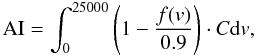 (1)where
f(v) is the normalized flux density. The value of
C is unity in contiguous intervals of width 450 km s-1 or
greater, over which the quantity in parentheses is everywhere positive; otherwise
C = 0. The AI was computed in C iv using an automatic procedure
in which equation 1 was applied where the continuum for the normalization was defined to be
the median intensity in the rest-frame spectral window 1440−1470 Å. Objects with
AI > 0 were selected as possible BAL QSO candidates.
(1)where
f(v) is the normalized flux density. The value of
C is unity in contiguous intervals of width 450 km s-1 or
greater, over which the quantity in parentheses is everywhere positive; otherwise
C = 0. The AI was computed in C iv using an automatic procedure
in which equation 1 was applied where the continuum for the normalization was defined to be
the median intensity in the rest-frame spectral window 1440−1470 Å. Objects with
AI > 0 were selected as possible BAL QSO candidates.
Each of the 536 spectra were examined by eye to identify any obvious wrong classifications due to, e.g., a poor estimate of the continuum derived from noise peaks or other features within the adopted spectral window. As a result of this combined automated and visual selection, we found 29 initial BAL QSO candidates.
Thirty of the QSOs with AI = 0 were randomly selected to build the control sample, with the requirement that their position in the sky was convenient for scheduling purposes in the various observing runs, and the distribution in redshift matched as closely as possible that of the BAL QSO sample.
These 59 QSOs form the sample of sources for which we obtained the multifrequency radio observations for this work.
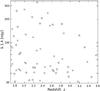 |
Fig. 1 Distribution in flux density and redshift, of the QSOs in both the BAL (crosses) and non-BAL (circles) samples. |
The sample of 25 radio-loud BAL QSOs studied in this paper.
The sample of 34 comparison (non-BAL) QSOs studied in this paper.
The above selection procedure, normalising the continuum to the intensity in a fixed wavelength range, is appropriate when dealing with large initial samples, but has two important caveats: (1) AI can be understimated if low-velocity absorption troughs are superimposed on the emission line, and (2) the assumption of a constant continuum over the region of interest may be inadequate for some sources. As a result, the control sample may include some QSOs that would be more appropriately classified as BAL QSOs, and vice versa. We measured the AI of the 59 QSOs more accurately using the following procedure. The continuum was obtained by interactively fitting the spectral region between the Si iv and the C iv emission lines (both included) with splines. After normalization with the fitted continuum, the C iv AI was measured using Eq. (1) but with the more strict definition of Trump et al. (2006), in which parameter C is unity over a contiguous interval of 1000 km s-1 rather than the 450 km s-1 used by Hall et al. (2002).
Of the total 59 QSOs, 25 have AI > 100 km s-1 according to this definition, and these form the final BAL QSO sample. This sample is shown in Table 1, where we provide the optical coordinates, redshifts (both from SDSS), AI, and peak flux densities at 1.4 GHz from FIRST. For 11 BAL QSOs with z ≤ 2.3, the SDSS spectra include the region in the vicinity of the Mg ii line at 2798 Å, allowing a search for the absorption in Mg ii that is characteristic of low-ionisation BAL quasars (LoBALs), as well as absorption in Fe ii (rest-frame range from 2200 to 2700 Å) characteristic of FeLoBAL quasars. Three of the sources display Mg ii absorption as well as Fe ii absorption and are therefore FeLoBALs, labelled “FeLo” in Table 1. The remaining 8 sources lack absorption from both Mg ii and Fe ii, and are identified as HiBAL and denoted “Hi” in Table 1. None of the 11 sources are LoBALs, showing Mg ii absorption but no Fe ii absorption.
Of the 29 QSOs initially selected as BAL QSOs, 1005+48, 1333+47, 1401+52, 1554+30, 2129+00, 2248−09, and 2331+01 have AI < 100 km s-1, and were therefore included in the comparison sample of non-BAL QSOs. In the opposite sense, 3 QSOs initially in the control sample have AI > 100 km s-1 and were re-classified as BAL QSOs, namely 1103+11, 1335+02, and 1404+07. The comparison sample is listed in Table 2. Figure 1 shows the distribution of the 59 QSOs in redshift and S1.4 flux density.
We note that the minimum velocity width we used for the selection of BAL QSOs, of 1000 km s-1, although well above the maximum expected values for galactic halos, of ~600 km s-1, is half the value used in the classical definition of BAL QSOs by Weymann et al. (1991), which identifies the most extreme cases, and was based on radio-quiet QSOs. Although a sample of extreme BAL QSOs might reveal more clearly the differences between the radio properties of BAL QSOs and a control sample of non-BAL QSOs, the fraction of BAL QSOs is lower among radio-selected samples than among optically selected ones, and moderate BAL QSOs have been included to ensure that there is a large enough sample for statistical studies. In addition, a more relaxed definition of broad absorption allows us to cover a wider range of outflow phenomena, including BALs with lower outflow velocities. These lower-velocity flows might be driven by different acceleration mechanisms, depending on the QSO radio luminosity (see Punsly 1999a, and references therein; and Ghosh & Punsly 2007, for BAL QSO models and its relation to radio emission). Using Weymann’s balnicity index (BI), defined as Eq. (1) apart from the lower velocity limit, which is chosen to be 3000 km s-1, and the above-mentioned wider absorption, >2000 km s-1, we obtained BI > 0 for 7 of the 25 BAL QSOs in this work, namely 0044+00, 0842+06, 1040+05, 1054+51, 1159+01, 1237+47, and 1624+37.
Summary of the observations.
Observing frequencies and beam sizes (half-power beam-width).
3. Radio observations and data reduction
We observed the QSOs at frequencies ranging from 1.4 to 43 GHz, using the 100-m Effelsberg single dish and the VLA in full polarisation mode (Stokes I, Q, and U images). Tables 3 and 4 summarise the different runs and observing setups.
3.1. Effelsberg 100-m telescope data
Observations with the Effelsberg 100-m dish were carried out during three separate runs (see Table 3). All observations (for BAL QSOs and comparison QSOs) were carried out using cross-scans in azimuth and elevation at 2.65, 4.85, 8.35, and 10.5 GHz, with a cross-scan length of four times the beam size. On-source integration times were between 20 and 60 s per source and per frequency, depending on the expected source intensity.
During the data reduction, all scans were visually checked to remove the radio-frequency interference, bad-weather effects (noisy scans due to heavy rain or clouds), or detector instabilities. The signals were fitted with a Gaussian to extract flux densities, following the standard reduction method for Effelsberg data, using the CONT2 programme of the TOOLBOX2 package. We derived 3-σ upper limits to the flux densities of undetected sources (Sect. 3.3).
The flux-densities were calibrated on the Baars et al. (1977) scale, using observations of 3C 286. A calibration of the polarisation was carried out in the standard way, using observations of 3C 286 to remove the effects of instrumental polarisation.
3.2. Very Large Array data
In July 2009, we used the VLA to observe the BAL QSOs in the frequency range 1.4 to 43 GHz. We used five different receivers (L, C, X, K, and Q band, corresponding to 1.4, 4.86, 8.46, 22.5, and 43.3 GHz) and imaged at all frequencies the QSOs in both the BAL QSO sample and the comparison sample. The integration times depended on both the band and source, and varied between 4 and 15 min.
The highest angular resolutions reached in our work are lower than those reached by MM08, since the latter used the VLA in its A configuration, whereas in this work we used its configuration C
The flux-densities were calibrated on the Baars et al. (1977) scale, via observations of 3C 286, which was also used as a phase calibrator. In addition, secondary phase calibrators were observed at regular time intervals (different for each band) and between two and five degrees from the target sources. At the highest frequencies (22 and 43 GHz), we switched between target and calibrator every 30 s (“fast-switching mode”), to improve the phase calibration.
The data were reduced with the 31DEC09 version of AIPS3, and version 3.0 of CASA4 was used to extract flux densities via an automated python script. We used the task IMSTAT to perform this calculation for the Stokes I, Q, and U images. We placed 3-σ upper limits on the flux densities of undetected sources (Sect. 3.3).
The polarisations were calibrated using 3C 286 as a strong unresolved source to determine the instrumental polarisation and the apparent polarisation angle.
3.3. Error determination
We followed the approach of Klein et al. (2003) to determine the flux-density errors, considering three main contributions: (i) the fractional calibration error ΔScal, estimated from the dispersion of the observations in the flux density calibrators; (ii) the error introduced by noise, ΔSn, which is estimated from the local noise around the source; and (iii) the confusion error ΔSconf due to the possible presence of background sources within the beam area. When the beam has small dimensions, as in interferometric data, the last term can be neglected.
Thus, the expressions for the total uncertainties in the Stokes parameters are given
by 2 and 3 for Effelsberg and VLA data, respectively  (2)
(2) (3)where
Asrc is the area of the aperture within which the source
flux density is measured, and Abeam is the area of the
synthesised beam. The expressions for the uncertainties in both m
(fractional polarisation) and χ (polarisation angle) can be found in
Klein et al. (2003).
(3)where
Asrc is the area of the aperture within which the source
flux density is measured, and Abeam is the area of the
synthesised beam. The expressions for the uncertainties in both m
(fractional polarisation) and χ (polarisation angle) can be found in
Klein et al. (2003).
4. Results and discussion
In Tables 5 and 6, we present our measurements of the flux densities of the BAL QSOs and the comparison sample from 1.4 to 43 GHz. For sources that were resolved in the VLA maps (see Sect. 4.1), we provide both the total flux densities and the flux densities of the individual components, where the components were well-resolved and when reliable measurements were possible. At 1.4 GHz, if we made no measurements, we give in Tables 5 and 6 the FIRST integrated flux densities. In the last column of each table, we give upper limits to the projected linear sizes of the unresolved sources, extracted from the highest-resolution VLA map with a significant detection. The sizes of resolved sources were obtained from whichever map had the largest projected linear size.
We extended the SEDs to frequencies lower than 1.4 GHz using data from the literature (see Table 7). Flux densities and upper limits (when cut-out images were available) were collected from the following surveys: VLSS (74 MHz, Cohen et al. 2007), 6C (151 MHz, Hales et al. 1988), WENSS (325 MHz, Bruyn et al. 2000), TEXAS (365 MHz, Douglas et al. 1996) and B3 (408 MHz, Ficarra et al. 1984).
4.1. Morphology
The radio morphologies of the QSOs in the two samples can be compared at the arcsec scale using the VLA maps, which have at all frequencies a higher resolution than the Effelsberg 100-m single-dish cross-scans. At 1.4 GHz, we complement our VLA data with those from FIRST data, obtained with a higher resolution. Maps of the resolved sources are shown in Fig. 2 and their linear sizes are listed in Tables 5 and 6.
The BAL QSO sample
Amongst the BAL QSO sample, 16 were detected at high angular resolution (3 with resolution 0.47 arcsec, from 43-GHz observations, and 15 with resolution 0.9 arcsec, from 22-GHz observations). Only one of them (1603+30) was resolved at either of these frequencies. Another five sources were observed with a poorer resolution, of 2.3 arcsec (8.46 GHz). For 0849+27, lacking VLA observations from our work, the FIRST data provide the highest resolution. A detailed discussion of the four resolved BAL QSOs is presented below.
 |
Fig. 2 Maps of the resolved QSOs. The synthesised beam size is shown in the lower left corner of the map. Levels are multiples of the 3-σ flux density value in mJy/beam, according to the legend. A cross indicates the SDSS optical position. |
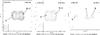 |
Fig. 2 continued. |
0816+48 is elongated to the south-west in the 1.4-GHz map. A Gaussian fit yields an
angular size of 29 arcsec along the major axis and an upper limit of 14 arcsec along the
minor axis, corresponding to a projected linear size of 217 kpc and
<105 kpc, respectively. The total spectral index in the range
from 4.86 to 8.46 GHz is 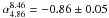 (see Sect. 4.4 and
Table 9).
(see Sect. 4.4 and
Table 9).
0849+27, for which we have no usable VLA observations, is resolved in the FIRST map
(resolution of 5 arcsec, see Fig. 2). The map shows
three components, located 25 arcsec northeast (NE) (D), 34 arcsec NE (B), and 20 arcsec
southwest (A) of the core (C), which is coincident with the QSO optical position. The four
components are included in the FIRST catalogue of radio sources. Throughout the paper, we
label core components as “C”. The largest separation between components is approximately
44 arcsec, corresponding to a projected linear size of 382 kpc. The total spectral index
of the source is  . If the two fainter and
farther away NE components were interpreted as a background source, 0849+27 would have a
size of 20 arcsec, corresponding to a projected linear size of 173 kpc.
. If the two fainter and
farther away NE components were interpreted as a background source, 0849+27 would have a
size of 20 arcsec, corresponding to a projected linear size of 173 kpc.
1103+11 is resolved at 1.4 (FIRST), 4.86, and 8.46 GHz, and shows a core-lobe morphology.
This interpretation is supported by the coincidence of component C with the optical
position of the QSO. The angular size from the highest-resolution map (8.46 GHz) is
8 arcsec, corresponding to a projected linear size of 69 kpc. The lobe is not detected at
higher frequencies, probably due to the steeper spectral index with respect to the core,
which decreases the lobe flux density below the 3-σ detection limit at
the highest frequencies. The spectral indices are  for the core (C) and
 for the lobe (A), and
 for the total emission.
1603+30 is resolved at 22 GHz, and has a core component (C) that is coincident with the
optical position of the QSO and another component towards the south (A), which could be
interpreted as a lobe. The angular size is 2 arcsec, corresponding to 17 kpc. The total
spectral index of the source is  .
.
The non-BAL QSO sample
For 31 of the 34 sources in the comparison sample, we obtained observations with resolutions 0.5 or 0.9 arcsec (frequencies 43 and/or 22 GHz) and for two other two sources we have 8.46-GHz observations with resolution 2.3 arcsec. The highest-resolution observations available for 2238+00 are from FIRST, and the source is unresolved. In total, four of the non-BAL QSOs are resolved:
-
1)
0033−00 has a core-lobe structure in the 8.46-GHz map. The total angular size is 6 arcsec (51 kpc) and the total spectral index is
 ;
; -
2)
a core-lobe structure is visible in 0125−00 at 4.86 and 8.46 GHz. Since at 4.86 GHz, the lobe is not well-resolved from the core, we only provide the total flux density (core and lobe) at this frequency in Table 6. The angular size, as measured from the 8.46 GHz map, is 5 arcsec, corresponding to 42 kpc. The total spectral index of the source is
 ;
; -
3)
1411+34 is resolved in the FIRST survey, and our VLA maps at 4.86 and 8.46 GHz show a core and double-lobe, with angular size at 8.46 GHz of 23 arcsec (199 kpc). At 22 and 43 GHz, only the core is detected. The spectral indices are
 for the core,
 for lobe A, and
 for lobe B. The total
spectral index is
for lobe B. The total
spectral index is  ;
; -
4)
1728+56 is a double source at 4.86 and 8.46 GHz. At 22 GHz, a core component is also detected, and is coincident with the optical position of the QSO. The B and C components, which are resolved at 22 GHz, are blended at the lower frequencies. The angular size (separation of A and B) at 22 GHz is 10 arcsec, corresponding to 87 kpc. The spectral index calculation for the A component yields
 and for B+C
 , indicating that the
lobe emission dominates. For the total emission, we found a spectral index
, indicating that the
lobe emission dominates. For the total emission, we found a spectral index
 .
.
In summary, we found from our multi-wavelength observations only eight resolved sources out of 59. The fractions of resolved sources in the two samples are similar, as are the ranges of angular sizes, from 20 to 200–400 kpc. The morphologies of the BAL QSOs include one extended source, two core-lobe, and an ambiguous case between core-lobe and core double-lobe. The morphologies of the non-BAL QSOs include two core-lobe and two core double-lobe sources. The fraction of unresolved sources is 21/25 = 84% for the BAL QSOs and 30/34 = 88% for the non-BAL QSOs. Twenty of the unresolved BAL QSOs and 27 of the unresolved non-BAL QSOs were observed at the VLA at 8.46 GHz, with 2.3 arcsec resolution. These data indicate that most of the QSOs in the two samples have sizes smaller than 20 kpc at 8 GHz, using the average redshift z = 2.4 of the two samples. Individual upper limits to the source linear sizes are given in Tables 5 and 6. Two of the unresolved BAL QSOs, 1159+01 and 1624+37, were resolved by VLBA (Montenegro-Montes et al. 2008b; in prep.), both showing a core-jet morphology with sizes of 0.85 kpc and 60 pc, respectively.
It has been suggested that up to 25% of the compact radio sources can intrinsically be extended sources, which are viewed as compact due to their orientation (Fanti et al. 1990). Our sample includes only QSOs, which are usually considered to be active galactic nuclei seen from a particular range of viewing angles, from a few degrees up to ~45° from the jet axis (limit imposed by the presence of the dusty torus). This, in principle, could increase the contamination, if we consider, as do Fanti et al., that a viewing angle <20°–30° can significantly reduce the projected linear size of a source.
4.2. Variability
For most of the sources, we have two measurements of the flux density at 4.8 GHz, one
from Effelsberg observations at 4.85 GHz and the other from the VLA at 4.86 GHz.
Similarly, at 8.4 GHz, we have for many sources Effelsberg data at 8.35 GHz and VLA data
at 8.46 GHz. We checked these flux densities for potential variable sources in the sample,
evaluating for each pair of measurements the fractional variability and significance. For
the sources resolved in the VLA maps (see Sect. 4.1), we used the total flux densities. We
adopted the fractional variability index defined by Torniainen et al. (2005)
 (4)The significance
of the source variability was estimated using the σVar
parameter defined e.g. by Zhou et al. (2006)
(4)The significance
of the source variability was estimated using the σVar
parameter defined e.g. by Zhou et al. (2006)
 (5)where
Si and
σi are the flux density and its
corresponding uncertainty. We consider as candidate variable sources those with
σVar ≥ 4 and a fractional variability ≥20%. In the
following, we briefly discuss these cases.
(5)where
Si and
σi are the flux density and its
corresponding uncertainty. We consider as candidate variable sources those with
σVar ≥ 4 and a fractional variability ≥20%. In the
following, we briefly discuss these cases.
In the BAL QSO sample, 20 sources have 4.8-GHz flux densities from both Effelsberg and the VLA, and 17 have 8.4-GHz flux densities (16 of these sources are in common with the first group). In four cases, we found σVar > 4 and we list in Table 8 the flux densities, variability significance, fractional variability, and time interval. None of these fractional variabilities exceeds 20%.
In the comparison sample, 30 sources were observed at 4.8 GHz by both telescopes, and 25 at 8.4 GHz. Seven of the sources have a variability significance of greater than 4 at one or both frequencies and are listed in Table 8. 1005+48 displays modest variability, just at the considered threshold. 0029−09 and 1521+43 both have a high variability significance, σVar > 10, and a high fractional variability, ~40–50 per cent, with 1521+43 being the most extreme case, showing large variations at the two frequencies. The remaining variable source, 1411+34, was resolved at the VLA (see Sect. 4.1). It shows variations at the two frequencies of the level of 20–40%, with significance 5–7σ. Since for this case, we found lower flux densities at the higher resolutions, the apparent variability of this source could be due to resolution effects, thus it cannot be considered a bona fide intrinsic variable candidate.
Summarizing the results from the comparison between VLA and Effelsberg data, we found that three sources are likely to have intrinsic variability, 0029−09, 1005+48, and 1521+43, all of them in the comparison sample. 1411+34 (non-BAL QSO sample) shows flux-density variations that could be due to resolution effects. Given the small number of variable sources, it is impossible to firmly state whether BAL and non-BALs have different variability behaviours, although our data suggest that the BAL QSO samples contains a lower fraction of variables.
The BAL QSOs 1159+01, 1603+30, and 1624+37 were also included in the MM08 sample. We studied the possible variability of these sources by comparing the flux densities at various frequencies in this work with those reported at MM08, considering the same radiotelescope (Effelsberg or VLA). Most of the flux densities for 1624+37 presented at MM08 were taken from Benn et al. (2005).
For 1159+01 we found that σvar > 4 in the comparison of VLA data at the frequencies of 8.4 GHz and 22 GHz, although in the first case yielding a low fractional variability, of 9%. At 22 GHz, the flux density variation is large, with σvar = 21 and fractional variability 60%. The variations could be due to resolution effects, since both correspond to an increase in flux density from the VLA A configuration data (HPBW = 0.08 arcsec) from MM08, to the lower resolution VLA C configuration data (HPBW = 0.9 arcsec) from this work. The flux densities varied from 160.8 ± 1.25 mJy to 176.6 ± 2.2 at 8.4 GHz, and from 105.5 ± 1.15 mJy to 169.2 ± 2.8 mJy at 22 GHz, in a time interval of 4.5 years.
For 1603+30, we were able to compare 2.6 and 4.8-GHz Effelsberg data, as well as 8.4 and 22-GHz VLA data. We found σvar = 4.9 and a fractional variability 49% for the 4.8-GHz Effelsberg data, over an interval of 4.5 years, indicating significant intrinsic variability. For the 8.4-GHz VLA data, there was a flux density variation from 22.1 ± 0.35 mJy at VLA(A) to 26.9 ± 0.6 mJy for VLA(C), in 3.4 years. The variation is significant, σvar = 6.9 and fractional variability 22%, although we cannot reject the possibility that resolution effects play a role. However, the variability at this frequency is confirmed by MM08, where the source is listed as a variable candidate (significance 4.2 and fractional variability 22%) based on the comparison between the flux densities from their data and those from Becker et al. (2000), both from the VLA in its A configuration.
Sources with significant variability, σVar > 4, from the observations in this paper.
For 1624+30, although the comparison of flux densities was possible at four frequencies (4.8 GHz from Effelsberg and 8.4, 10.5 and 22 GHz from the VLA), none of them yielded σvar > 4. Therefore, from the comparison with the flux densities in MM08, only 1603+30 is a candidate variable.
In total, four sources, one BAL QSO and three non-BAL QSOs, are classified as intrinsic variables (not due to resolution effects) at levels above 20% (0029−09, 1005+48, 1521+43, and 1603+30). The additional data from MM08 weaken the trend of BAL QSOs being less variable than non-BAL QSOs.
Barvainis et al. (2005) studied the flux density
variability at 8.4 GHz over ten epochs (the measurement interval for each source ranging
from two weeks to 1.6 years) of a core-dominated sample of 50 QSOs with
S8.4 GHz ≥ 0.3 mJy, including radio-quiet, radio-loud, and
radio-intermediate QSOs. Thirty-eight of the QSOs in their sample (76%) have a flat radio
spectrum, with  . The authors found five
QSOs with fractional variability above 20%, four in the range 20–40% and one with
fractional variability of 140%. The four QSOs with higher variability have flat spectra,
whereas the remaining one is steep. The fraction of sources varying by at least 20% found
by Barvainis et al. (2005) (5/50) is consistent with
our results for the SDSS-FIRST QSOs (4/59), within the errors. In addition, we show in
Sect. 4.4 that the variable sources in our work also tend to have a flat spectrum in the
frequency range from 5 to 8 GHz, although our sample has a smaller fraction of
flat-spectrum sources (25/59 = 42%, see Sect. 4.4 and Table 9, compared to 76% in Barvainis et al. 2005, sample). This smaller fraction of flat-spectrum sources could also explain
the slightly smaller fraction of variables that we identify here.
. The authors found five
QSOs with fractional variability above 20%, four in the range 20–40% and one with
fractional variability of 140%. The four QSOs with higher variability have flat spectra,
whereas the remaining one is steep. The fraction of sources varying by at least 20% found
by Barvainis et al. (2005) (5/50) is consistent with
our results for the SDSS-FIRST QSOs (4/59), within the errors. In addition, we show in
Sect. 4.4 that the variable sources in our work also tend to have a flat spectrum in the
frequency range from 5 to 8 GHz, although our sample has a smaller fraction of
flat-spectrum sources (25/59 = 42%, see Sect. 4.4 and Table 9, compared to 76% in Barvainis et al. 2005, sample). This smaller fraction of flat-spectrum sources could also explain
the slightly smaller fraction of variables that we identify here.
Sadler et al. (2006) investigated the variability
at 20 GHz over one to two years of a sample of radio sources selected to have
S20 GHz ≥ 100 mJy and including 32 QSOs. The QSO
sub-sample is dominated by flat-spectrum sources (69% with
 ) and has two sources just
above the 20% fractional variability threshold (2/32). Although the number of sources in
this sample is small, the proportion of variable sources is consistent with that found by
Barvainis et al. (2005) and in this work. We note
however that the two QSOs in Sadler et al. (2006)
that have a variability above 20% do not have flat spectra (their spectral indices being
) and has two sources just
above the 20% fractional variability threshold (2/32). Although the number of sources in
this sample is small, the proportion of variable sources is consistent with that found by
Barvainis et al. (2005) and in this work. We note
however that the two QSOs in Sadler et al. (2006)
that have a variability above 20% do not have flat spectra (their spectral indices being
 and
and
 ).
).
4.3. Shape of the radio spectra
With the collected multi-frequency data, it is possible to study the shape of the synchrotron emission of the quasars in the two samples, allowing us to obtain the fraction of CSS-GPS sources. The GPS sources are compact (≤ 1 kpc) and have a convex radio spectrum that peaks between 500 MHz and 10 GHz in the observer’s frame, CSS are larger (between 1 and 20 kpc in size) and have convex spectra that tend to peak at lower frequencies, of typically <500 GHz (O’Dea 1998). The SEDs of the sources are shown in Fig. 3 as log Sν versus logν plots, using the flux densities listed in Tables 5–7. For resolved sources, we used the total flux densities.
We fitted the spectral energy distributions (SEDs) of the sources with observations at several frequencies, via χ2 minimization, with a power-law model (L) and a parabola (P), on the log Sν versus log ν plane. A fit was accepted as statistically significant if the parameter Q, indicating the probability that a value of χ2 as poor as the value found should occur by chance, was above 0.01. The parabolic model was chosen as a simple representation for the curved SEDs in the log Sν versus (vs.) logν plane, following Kovalev (1996). For the cases where both models were statistically acceptable, the power law was selected as the best fit. The fits are shown in Fig. 3 using a dashed line for the power-law model and a continuous line for the quadratic model.
For a total of ten sources (BAL QSOs 0842+06, 0849+27, 1014+05, 1229+09, and 1304+13, and non-BAL QSOs 0033−00, 1401+52, 2109−07, 2248−09, and 2353−00), we found statistically significant fits as power laws, and these sources are labelled as LQ in Table 9, where the fitting results are presented. For six further sources, we found a statistically significant fit for the parabolic model (BAL QSOs 1054+51, 1102+11, 1337−02, and 1603+30, and non-BAL QSOs 0154−00 and 1636+35). All these fits are convex, i.e. display a flattening from high (10–20 GHz) to mid (1–5 GHz) frequencies. These sources are labelled PQ in Table 9. Although BAL QSO 1159+06 also falls in this category, we adopted the linear model for this source, since the peak of the parabola is far away from the observed frequencies, the linear and parabolic model being practically coincident over the observed range. We adopt the label L in Table 9 for this source.
For the other 29 sources at least one of the models shows a good match from visual inspection, and we selected as the best model the one yielding the lowest mean squared error, labelling the sources as L or P in Table 9. The linear model includes six sources (BAL QSO 1327+03 and non-BAL QSOs 0029−09, 0152+01, 0158−00, 1322+50, and 1512+35), and the parabolic model 15 sources (BAL QSOs 0044+00, 0756+37, 1129+44, 1237+47, 1404+07, and 1624+37 and non-BAL QSOs 0103−111, 0750+36, 1411+43, 1641+33, 2129+00, 2143+00, 2244+00, 2331+01, and 2346+00), all of them with a convex shape. Although the remaining eight sources are those with the smallest mean squared errors for the quadratic model, we adopted the linear fit, which similarly had a small mean squared error, because either the peak was far away from the SED, making the linear and quadratic models very similar, or the parabolic shape was concave, which is inconsistent with the expected shapes from synchrotron models. As for 1159+06, described in the previous paragraph, we used the italic label L for these sources (BAL QSOs 1103+11 and 1335+02, and non-BAL QSOs 0124+00, 0125−00, 1502+55, 1521+43, 1528+53, and 1728+56). For the sources modelled with a parabola, with its peak within the fitted range, the frequency peaks are listed in Table 9.
Another three sources were not fitted, since they showed abrupt changes in their SEDs (BAL QSOs 0816+48 and 0905+02, and non-BAL QSO 1333+47).
Another eight sources (BAL QSOs 0929+37, 1159+01, 1406+34, and non-BAL QSOs 0014+01, 1005+48, 1411+34, 1554+30, 1634+32) have SEDs that suggest the presence of a separate component at low frequency. The source 1411+34 was also morphologically resolved as a core double-lobe whose two lobes were steeper, i.e. stronger at low frequencies, than the core (see Sect. 4.1). For these sources, we considered fits removing one or various lowest-frequency data points with hints of excess emission. The low-frequency points rejected from the fits are indicated in Table 9. Regarding the high-frequency components, six of the sources belong to class P and another one to class PQ, which all have convex shapes. The SED of 1159+01 shows hints of excess emission from 325 MHz to 1.4 GHz, leaving only three high-frequency data points. Since the power-law fit gives a low mean squared error, we adopted this model for the source. For the cases where the high-frequency component was modelled as a parabola with its peak within the fitted range, the frequency peaks are listed in Table 9, using italic digits. However, these sources cannot be considered as CSS-GPS candidates, because of the presence of the secondary low-frequency emission.
The remaining sources in the sample are 1040+05 (BAL QSO) and 2238+00. For 1040+05 only three data points were available, with an obvious flattening at low frequencies, and we selected as a best-fit model a parabola passing through these points. 2238+00 has a good quality measurement at only one frequency.
In total, we found 9 BAL QSOs and 16 non-BAL QSOs whose complete SEDs are consistent with power laws. For 11 BAL QSOs and 11 non-BAL QSOs, the fits indicate a curved shape along the whole SED due to a flattening of the spectra at low frequencies. For 15 of these (eight BAL QSOs and seven non-BAL QSOs), the frequency peak of the model parabola falls within the fitted range, with values ranging from 500 MHz to 7 GHz in the observer frame, indicating that they represent candidate GPS sources. Three sources that were not fitted owing to abrupt changes in their SEDs, have maxima within the observed frequency range and frequency peaks above 1 GHz. In addition, although BAL QSO 1129+44 is fitted with a parabola whose peak is below the observed frequency range, the flux-density distribution has a peak at 2.6 GHz. Among these 19 sources whose SED is GHz-peaked, two are resolved, BAL QSOs 0816+48 and 1603+30, with sizes of 217 kpc and 17 kpc, respectively (see Sect. 4.1), exceeding the limit of 1 kpc for GPS sources (O’Dea 1998). Excluding these two sources, the total number of candidate GPS sources would be 9 BAL QSOs and 8 non-BAL QSOs, with corresponding fractions with respect to the total samples of 36 ± 12% (9/25) and 23 ± 8% (8/34), adopting Poisson errors. In Sect. 4.1, we obtained for the unresolved sources a conservative upper limit of 20 kpc for their sizes at 8.4 GHz, therefore higher-resolution observations are needed to confirm their GPS classification. In particular, this classification is confirmed for 1624+37, with a size of 60 pc at 5 GHz and 75 pc at 8 GHz (Montenegro-Montes et al. 2008b; in prep.). The fractions of GPS candidates in the BAL QSO and non-BAL QSO samples are similar, within the errors. Considering the interpretation that GPS sources are young, our result suggests that BAL QSOs are no younger than non-BAL QSOs.
We adopted a conservative approach for the identification of young objects, since only candidate GPS sources were considered. However, we note that CSS objects displaying a steep spectrum in the GHz frequency range, with peak frequencies below 500 MHz, can be interpreted as young sources. Additional observations at low frequency could confirm the presence of peaks in the MHz frequency range for some of the sources in this work. The maximum size for CSS is 20 kpc (O’Dea 1998) and most of the sources in this work are unresolved having sizes below this limit.
The fraction of QSOs with hints of an additional low-frequency component (up-turn at low frequency) is 12 ± 7% for BAL QSOs (3/25) and 15 ± 7% for non-BAL QSOs (5/34), the two values being similar within the errors. Since this low-frequency excess emission likely corresponds to old components, this result again favours similar ages for BAL and non-BAL QSOs.
4.4. Spectral indices
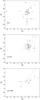 |
Fig. 4
|
The distribution of radio spectral indices constrains the distribution of orientations for a given population of radio sources (Orr & Browne 1982), since flatter spectral indices are indicative of lines of sight closer to the radio axis. Spectral indices of the QSOs were computed in the observed frequency intervals 4.8–8.4 GHz and 8.4–22 GHz, since these frequencies exceed the typical peak frequencies of the candidate GPS sources in the sample. We used the total flux densities for the resolved sources and VLA data, which were obtained during a one-week run (see Table 3). Effelsberg flux densities were adopted for the few sources/frequencies lacking VLA data (BAL QSOs 0849+27 and 1229+09 and non-BAL QSOs 0154−00 and 1636+35). The spectral indices and their errors are listed in Table 9.
Figure 4 (top and middle panels) show
 versus
 for the two
samples. The square symbols correspond to sources without available spectral indices
. They were
plotted using the mean of each
sample. Upper limits are plotted as triangles. The dotted line traces pure power-laws: the
location of most of the sources below this line is due to the steepening at high
frequencies. The spectral indices of the BAL QSOs show a large scatter in the plot.
Although most BAL QSOs are found in the same region as non-BAL QSOs, there is an apparent
excess of steep sources in the BAL QSO sample, with six sources having spectral indices
smaller than −1.5 in either of the two frequency ranges. In addition, there appears to
be an excess of non-BAL QSO sources with
for the two
samples. The square symbols correspond to sources without available spectral indices
. They were
plotted using the mean of each
sample. Upper limits are plotted as triangles. The dotted line traces pure power-laws: the
location of most of the sources below this line is due to the steepening at high
frequencies. The spectral indices of the BAL QSOs show a large scatter in the plot.
Although most BAL QSOs are found in the same region as non-BAL QSOs, there is an apparent
excess of steep sources in the BAL QSO sample, with six sources having spectral indices
smaller than −1.5 in either of the two frequency ranges. In addition, there appears to
be an excess of non-BAL QSO sources with  .
However, when the distributions of spectral indices for the BAL and non-BAL QSO samples
are compared using the Kolmogorov-Smirnov (K-S) test, they are found to differ only at a
significance level of 74% for and 0.3%
for . We also
tested the hypothesis that the distribution of spectral indices is steeper for BAL QSOs
than for non-BAL QSOs: the significance levels increase to 87% for
and 28% for
. Finally,
the hypothesis that the SEDs of BAL QSOs are flatter than those of non-BAL QSOs can be
rejected at a 100% confidence level for and at a
77% confidence level for .
.
However, when the distributions of spectral indices for the BAL and non-BAL QSO samples
are compared using the Kolmogorov-Smirnov (K-S) test, they are found to differ only at a
significance level of 74% for and 0.3%
for . We also
tested the hypothesis that the distribution of spectral indices is steeper for BAL QSOs
than for non-BAL QSOs: the significance levels increase to 87% for
and 28% for
. Finally,
the hypothesis that the SEDs of BAL QSOs are flatter than those of non-BAL QSOs can be
rejected at a 100% confidence level for and at a
77% confidence level for .
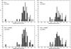 |
Fig. 5 Distribution of the radio spectral indices ( |
Although we do not find any statistical evidence of steeper spectra for BAL QSOs, we can firmly exclude that BAL QSOs have on average flatter radio spectra than non-BAL QSOs, in the frequency range 4.8–8.4 GHz.
Figure 4 (bottom panel) shows the same spectral index diagram for the BAL QSOs in MM08.
The BAL QSOs 1159+01, 1603+30, and 1624+37, which are common to both samples, were plotted
with a different symbol (circles with their size increasing with the right ascension of
the sources). From the combined sample of BAL QSOs in this work and MM08 (using our data
for the sources in common), we find that the hypothesis that BAL QSOs have a steeper
than
non-BAL QSOs has a higher confidence level of 91%, although still below the threshold of
95% generally adopted for the rejection of the null hypothesis. In this test, we note that
we are using the comparison sample selected for this work, with
S1.4 > 30 mJy, which is brighter
than the 15-mJy limit of MM08. Regarding , the
combined sample of BAL QSOs has steeper spectra than the non-BAL QSO sample only at a 55%
confidence level. The hypothesis that the BAL QSOs in the combined sample have flatter
spectra than non-BAL QSOs can be rejected at a 97% confidence level
for and at a
98% confidence level for .
Although the evidence of steeper spectra for BAL QSOs is at best marginal, with a 91% significance for the test between the combined BAL sample and the comparison sample at the frequency range 4.8–8.4 GHz, we can reject with a high confidence, above 97%, that BAL QSOs have on average flatter radio spectra than non-BAL QSOs, in both of the frequency ranges 4.8–8.4 GHz and 8.4–22 GHz. We interpret this result as statistical evidence that the BAL QSOs in our sample, or in combination with MM08 sample, do not tend to have position angles closer to the radio axis than non-BAL QSOs, i.e. the orientation models for BAL QSOs in which they predominantly arise from polar winds (for instance Punsly 1999a,b), contradict our results. At a lower level of significance, the slightly steeper spectra of BAL compared to those of non-BAL QSOs in the range 4.8–8.4 GHz are consistent with the equatorial wind model of Elvis (2000).
Figure 5 shows histograms of the distributions of and
for the BAL
and non-BAL QSO samples, and statistics are presented in Table 10. The spectral indices in
the two frequency ranges show a mixture of flat (α ≥ −0.5) and steep
(α < −0.5) spectra for the BAL and non-BAL
QSO samples (see also Table 9). The values found
for BAL QSOs suggest that these QSOs are seen from a wide range of orientations with
respect to the jet axis (both flat and steep sources being present). The same conclusion
that BAL QSOs are not orientated along a particular line of sight was obtained by Becker
et al. (2000) and MM08, also on the basis of the
radio spectral indices of BAL QSOs. The comparison in our work with a control sample
similar in redshift and both radio and optical properties, except for the absence of broad
absorption features, reveals a weak tendency for BAL QSOs to be on average steeper than
non-BAL QSOs, and allow us to firmly conclude (above 97% confidence) that BAL QSOs do not
have flatter spectra than non-BAL QSOs.
The two spectral-index distributions obtained for the FIRST-SDSS QSOs in our work, and for the BAL QSO sample by MM08, can be compared to those reported in the literature for other samples of radio QSOs. A useful comparison is with the B3-VLA QSO sample (Vigotti et al. 1997, 1999), which was selected at 408 MHz and is complete down to S = 100 mJy, with multi-frequency data available from which we can compute the spectral index in the range 4.8–10.6 GHz, close to the range 4.8–8.4 GHz used in the present work. The angular sizes at 1.4 GHz of the B3-VLA QSOs were measured from maps taken with the VLA in C and D configurations (Vigotti et al. 1989) and for the most compact sources from observations in A configuration (private communication). Since most of the QSOs in our sample are unresolved, as well as analysing the spectral-index distribution for the B3-VLA QSO sample as a whole (largest angular size 131 arcsec), we also considered a subsample with angular sizes below 2.3 arcsec, which is a representative upper limit to the sizes of the unresolved sources in our work (from 8.46-GHz VLA data).
Statistics for the spectral indices  of the
B3-VLA QSOs are included in Table 10, which
considers the whole sample and the sub-sample of more compact sources, with sizes below
2.3 arcsec. A K-S test shows that the spectral-index distribution of the compact B3-VLA
and BAL QSOs are similar at the 97% confidence level, for both the sample reported here
and the combined sample including MM08 BALs. The comparison with non-BALs shows that
B3-VLA QSOs are steeper, at a 99.1% confidence level. There is no obvious physical reason
for B3-VLA QSOs to be more similar to BAL QSOs than to non-BAL QSOs, the most plausible
explanation being that the selection of B3-VLA QSOs at a low frequency, 408 MHz, favours
the inclusion of sources with steeper spectra. That the spectral indices of B3-VLA QSOs
are more similar to those of BAL QSOs than to those of non-BAL QSOs is a consequence of
the SEDs of the former being slightly steeper than the latter. Furthermore, this result
emphasizes the importance of using an appropriate control sample.
of the
B3-VLA QSOs are included in Table 10, which
considers the whole sample and the sub-sample of more compact sources, with sizes below
2.3 arcsec. A K-S test shows that the spectral-index distribution of the compact B3-VLA
and BAL QSOs are similar at the 97% confidence level, for both the sample reported here
and the combined sample including MM08 BALs. The comparison with non-BALs shows that
B3-VLA QSOs are steeper, at a 99.1% confidence level. There is no obvious physical reason
for B3-VLA QSOs to be more similar to BAL QSOs than to non-BAL QSOs, the most plausible
explanation being that the selection of B3-VLA QSOs at a low frequency, 408 MHz, favours
the inclusion of sources with steeper spectra. That the spectral indices of B3-VLA QSOs
are more similar to those of BAL QSOs than to those of non-BAL QSOs is a consequence of
the SEDs of the former being slightly steeper than the latter. Furthermore, this result
emphasizes the importance of using an appropriate control sample.
The QSO sample from our work includes four sources classified as variable: the unresolved
non-BALs 0029−09, 1005+48, and 1521+43 and the resolved BAL QSO 1603+30. We note that
0029−09 and 1521+43 are the flattest sources in the total QSO sample, both with
 . The
resolved BAL QSO 1603+30 has a spectral index near the limit between flat and steep
spectra (
. The
resolved BAL QSO 1603+30 has a spectral index near the limit between flat and steep
spectra ( ). 1005+48 displays a
modest variability (just at the adopted thresholds of significance and fractional
variability) and its spectral index is
). 1005+48 displays a
modest variability (just at the adopted thresholds of significance and fractional
variability) and its spectral index is  . This trend between
variability and a flat radio spectra is consistent with the expectation that a flat
spectrum source is more likely to experience Doppler beaming, and therefore have any
existing variability magnified by this same effect.
. This trend between
variability and a flat radio spectra is consistent with the expectation that a flat
spectrum source is more likely to experience Doppler beaming, and therefore have any
existing variability magnified by this same effect.
The rest-frame radio luminosities of the sources, L4.8 GHz
are listed in the penultimate column of Table 9.
They were calculated using the total flux density at 4.86 GHz from the VLA or from
Effelsberg if VLA data were unavailable from this work. The k-correction was obtained
using the spectral index listed in
the same table. The radio luminosities range from 1026.1 to 1028.6,
above the limit Lrad = 1026 W Hz-1
generally adopted for radio-loud QSOs (Miller et al. 1990).
4.5. Polarisation
Fractional polarisation m (in percentage), at several frequencies (ν in GHz), for the BAL QSO sample.
For all sources, we derived SQ and SU to calculate the fractional polarisation m and the polarisation angle χ. Most of the measurements were obtained from the VLA observations. In only a few cases did the Effelsberg observations have a sufficiently high signal-to-noise ratio to detect polarisation fractions below 10%. Only 3-σ results were considered, except for the cases for which a detection above 2-σ resulted in a consistent m with respect to the other frequencies, increasing the measurement reliability. Values of the fractional polarisation are presented in Tables 11 and 12 for BAL and non-BAL QSOs, respectively. We included the NVSS values (NRAO VLA Sky Survey, Condon et al. 1998) for the polarisation fraction at 1.4 GHz when no measurements could be obtained from our data. The polarisation measurements as well as the more significant upper limits were mostly obtained for frequencies in the range from 1.4 to 8.5 GHz.
We obtained the cumulative distribution function F(m) = Prob(M ≤ m) for the fractional polarisation at 1.4, 4.8, and 8.4 GHz for the two samples, using the Kaplan-Meier estimator, that allows inclusion of information from upper-limits. The method is described in detail in Feigelson & Nelson (1985). The results are shown in Fig. 6. The pair of numbers in parenthesis indicates the number of detections and the number of upper limits for each frequency.
The distributions for the non-BAL QSOs are very similar for the three frequencies, yielding a median value m in the range 1.8–2.5%. The 85% percentile corresponds to m ≤ 5.8 −6.3%. Table 12 shows five sources exceeding m = 10% at some frequency. These sources are 0014+01, 0124+00, 0152+01, 1005+48, and the lobe component of 0125−00. In particular, 1005+48 shows fractional polarisation above 10% at a wide range of frequencies, from 2.6 to 22 GHz. The distributions for the BAL QSOs have a larger uncertainty, owing to the fewer data points and the larger fraction of upper limits, especially at 4.8 and 8.4 GHz. From the 1.4 GHz data, we find a median m = 1.8% and a limit m ≤ 6.2% for the 85% percentile. None of the measurements in Table 11 are above m = 10%.
Regarding the three BAL QSOs in common with MM08, we note that for 1603+30 these authors obtained m = 1% at 8.4 GHz and upper limits for the remaining frequencies in their study. For this source, we only obtained upper limits, and the one at 8.4 GHz is consistent with the measurement at MM08. For 1159+01, our measurements at 4.8 and 8.4 GHz agree with the results by MM08, although at 1.4 GHz we obtained m = 6%, less than half the value reported by MM08, of m = 15% (taken from NVSS). For the remaining source, 1624+37, our data only provide a high upper limit for m, but the source shows a high fractional polarisation from the data reported in Benn et al. (2005, their Table 2), with m = 6% at 4.8 GHz and m = 11% at 10 and 22 GHz.
The fractional polarisations of BAL and non-BAL QSOs appear to be similar, with median values around 1–3%, 85% of the sources having m < 6% and around ten per cent of the sources showing fractional polarisation above 10% at some frequency (4/34 for the non-BAL QSOs and 2/25 for the BAL QSOs, considering the information from the literature).
An extensive survey of the fractional polarisation of QSOs is presented in Pollack et al.
(2003), based on a sample with
S4.85 GHz ≥ 350 mJy and radio spectral index
 . The authors computed
m at 4.85 GHz separately for the core and jet components, and found a
higher polarisation for the jet components. In particular, the 85% percentile corresponds
to m ≤ 3% for the core components and to m ≤ 14% for the
jet components, and the proportion of sources exceeding a fractional polarisation of 10%
is 1/91 for the cores and 17/43 for the jet components. The fractional polarisations we
found for the BAL and non-BAL QSOs in our sample occupy an intermediate range between the
results found by Pollack et al. (2003) for core and
jet components.
. The authors computed
m at 4.85 GHz separately for the core and jet components, and found a
higher polarisation for the jet components. In particular, the 85% percentile corresponds
to m ≤ 3% for the core components and to m ≤ 14% for the
jet components, and the proportion of sources exceeding a fractional polarisation of 10%
is 1/91 for the cores and 17/43 for the jet components. The fractional polarisations we
found for the BAL and non-BAL QSOs in our sample occupy an intermediate range between the
results found by Pollack et al. (2003) for core and
jet components.
Sadler et al. (2006) obtained the polarisation
fraction or upper limits for 41 QSOs in their sample of radio sources selected at 20 GHz,
with S20 GHz ≥ 100 mJy. As mentioned in Sect. 4.2, this QSO
sub-sample is dominated by flat-spectrum sources (69% with
, compared to 42% for the
SDSS-FIRST QSOs in our sample). We obtained the cumulative distribution function of
m for this sample, using the Kaplan-Meier estimator, and found
m = 2.4% and m ≤ 4.2% for the median and the 85%
percentile, respectively. None of the QSOs in the Sadler et al. (2006) sample exceed polarisation levels of 10%. The results of Sadler
et al. (2006) show good agreement with those of
Pollack et al. (2003) for the core components.
4.6. Rotation measures
With at least three measurements of the polarisation angle χ at different frequencies, it is possible to estimate the rotation measure (RM) of a source, via a linear fit of the polarisation angle versus the square of the observed wavelength λ (χ = χ0 + RMλ2, χ0 being the intrinsic polarisation angle). The rotation measure, which is the slope of the fit, is proportional to the magnetic field component along the line of sight, to the electron density, and to the path length,
 (6)Plots of the
linear fits for the four BAL QSOs and ten non-BAL QSOs with at least three measurements
are shown in Fig. 7. The observed RM values are listed in Tables 11 and 12, along with the RM
values corrected from the Galaxy contribution and converted to the rest-frame, multiplying
by the factor (1 + z)2. Since the sources are located well
above the Galactic plane (b > 28°) the
applied Galactic correction was small, in the range from −9 to 17 rad m-2
(Taylor et al. 2009).
(6)Plots of the
linear fits for the four BAL QSOs and ten non-BAL QSOs with at least three measurements
are shown in Fig. 7. The observed RM values are listed in Tables 11 and 12, along with the RM
values corrected from the Galaxy contribution and converted to the rest-frame, multiplying
by the factor (1 + z)2. Since the sources are located well
above the Galactic plane (b > 28°) the
applied Galactic correction was small, in the range from −9 to 17 rad m-2
(Taylor et al. 2009).
There is good agreement between the observed rotation measure for 1159+01 in this work, of 79.2 ± 1.8 and the result from MM08, of 72.1 ± 1.4. The RM listed in Table 11 for 1624+37 was taken from Benn et al. (2005). With a rest-frame RM of 18 350 ± 570 rad m-2, this was and still is the second-highest RM known, after that of quasar OQ172 (Kato et al. 1987; O’Dea 1998), with RM = 22 400 rad m-2.
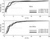 |
Fig. 6 Cumulative distribution of the fractional polarisation for the two samples, at each of three frequencies. Each pair of numbers in parenthesis indicates the number of detections and the number of upper limits at that frequency. The dashed lines indicate the 50% percentile (i.e. the median) and the 85% percentile. |
For the non-BAL QSO sample, we have data available for ten sources, allowing some statistical analysis. We found rest-frame |RM| values in the range from 8.7 to 3077 rad m-2, with a median value of 883 rad m-2, and an average and a standard deviation of 1180 rad m-2 and 1117 rad m-2, respectively. Three of the BAL QSOs have rest-frame |RM| values within the range found for the non-BAL QSOs. One of the remaining BAL QSOs with available rotation measure is 1406+34, with RM = 3520 ± 57 rad m-2, which is only 2σ from the average value for the non-BAL QSOs. The other source is 1624+37, with the extremely high value RM = −18350 ± 570. The small number of data points for BAL QSOs does not allow us to compare the rotation measures of the two samples.
Zavala & Taylor (2004) reported rest-frame rotation measures, |RM|, for the flat core components of 26 QSOs in the range from 200 to 10 000 rad m-2, with a median value of 1862 rad m-2 and average 2515 rad m-2. The same authors found lower values for the rotation measures of the steep jet components of these QSOs, namely a median value of 458 rad m-2 and average 600 rad m-2. The statistics for the non-BAL QSOs in our sample places them in the intermediate range of rotation measures between those of the flat and steep components in Zavala & Taylor (2004) sample.
5. Conclusions
We have constructed a sample of 59 radio-loud QSOs with S1.4 > 30 mJy, selected by cross-correlating the FIRST radio survey and the fourth edition of the SDSS Quasar Catalogue, at redshifts such that the wavelength range from Si iv 1400 Å to C iv 1550 Å is covered by the SDSS spectra. The sample comprises 25 sources with definite broad absorption in C iv and a velocity width of at least 1000 km s-1, referred to as the “BAL QSO sample”, and 34 sources lacking this absorption, which form the “non-BAL QSO comparison sample”. The sources were observed at frequencies ranging from 1.4 to 43 GHz, using the 100-m Effelsberg telescope and at the VLA, and these have allowed us to compare several radio properties of the two samples, including morphology, flux-density variability, spectral shapes, spectral-index distributions, and polarisation properties.
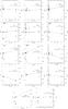 |
Fig. 7 Linear fits of the polarisation angles χ versus the square of the observed wavelengths for 4 BAL QSOs and 10 non-BAL QSOs, yielding the rotation measures. The errors in the position angles are lower than the dot size. Triangles correspond to the polarisation percentages (m). |
5.1. Linear sizes
Only 8 of the 59 sources are extended at the arcsec level, four of them being BAL QSOs and 4 of them non-BAL QSOs. The fractions of resolved sources are similar for BALs (16%) and non-BALs (12%), and the distributions of linear sizes are also similar, ranging from 20 to 200–400 kpc. The morphologies are also similar, including elongated sources (1), core-lobe (4, possibly 5) and core double-lobe (2, possibly 3). About 90–95% of the unresolved sources have an estimated size at 8.46 GHz below 20 kpc, as inferred from VLA observations at this frequency (2.3 arcsec resolution), and adopting the average redshift z = 2.4 for the two samples. Two of the unresolved BAL QSOs, 1159+01 and 1624+37, were resolved from VLBA observations at Montenegro-Montes et al. (2008b; in prep.), both showing a core-jet morphology and sizes of 0.85 kpc and 60 pc, respectively.
5.2. Flux density variability
The flux density variability of the sources at 4.8 GHz and 8.4 GHz was computed from observations at VLA and Effelsberg, at the same frequency, in two epochs separated typically by 1.6 years. In addition, for the 3 BAL QSOs in common with MM08, the flux densities from our work at various frequencies in the interval 2.6–22 GHz (VLA or Effelsberg) were compared to similar data (frequency and telescope) from MM08, with a time difference of 3–4 years. Excluding variations that could be attributed to resolution effects (higher flux at the lower angular resolution for any source, regardless of whether they are resolved), we found three likely variables from our data, which are all non-BAL QSOs (0029-09, 1005+48, 1521+43). Using flux densities from the literature, we concluded that the BAL QSO in our sample 1603+30 was also a candidate variable. Our data suggest that there is a lower rate of variable sources among BAL than non-BAL QSOs. However, this needs to be confirmed by monitoring the sample at various epochs using the same telescope configuration.
The proportion of variable sources exceeding a fractional variability of 20% in our total sample, 4/59, is consistent with the fraction for the core-dominated QSO sample of Barvainis et al. (2005), selected at 8 GHz and yielding a fraction of 5/50 variables at this frequency. The proportion is also consistent with the fraction 2/32 from the QSO sample studied at 20 GHz by Sadler et al. (2006).
5.3. Radio spectral shape
We found 9 BAL QSOs and 8 non-BAL QSOs with GPS-like radio spectra, having peak frequencies in the range from 0.5 to 7 GHz in the observer frame. Their linear sizes (or limits thereon, typically 20 kpc at 8 GHz) are consistent with a maximum allowed size of 1 kpc, for classification as a GPS source. Higher-resolution observations are needed to confirm or reject the GPS classifications of these sources. In particular, this classification is confirmed for 1624+37, with a size of 60 pc at 5 GHz and 75 pc at 8 GHz (Montenegro-Montes et al. 2008b; in prep.).
The fractions of candidate GPS sources are 36 ± 12% (9/25) for BAL QSOs and 23 ± 8% (8/34) for non-BAL QSOs, i.e. no significant difference. Given the widespread interpretation that GPS are young sources, our result suggests that BAL QSOs are no younger than non-BAL QSOs.
Low-frequency upturns in some of the radio spectra indicate that there are additional low frequency components, in about 12 ± 7% of the BAL QSOs (3/25) and 15 ± 7% of the non-BAL QSOs (5/34). The two values are similar within the errors, and since the low-frequency excess emission likely corresponds to old components, this result again implies that BAL and non-BAL QSOs have similar distributions of ages.
5.4. Radio spectral indices
We found a mix of flat (α ≥ −0.5) and steep
(α < −0.5) spectra for both the BAL and
non-BAL QSO samples, suggesting that both classes are seen from a wide range of
orientations with respect to the jet axis. A similar conclusion was reached by Becker
et al. (2000) and MM08, based on the radio
spectral-index distribution of BAL QSOs. Statistical tests comparing the spectral index
distribution of the two
samples provide weak evidence (at the 91% confidence level) that the spectra in the
combined BAL QSO sample from our work and MM08 are steeper than those in the non-BAL QSO
sample, and significant evidence (≥97% confidence) that the SEDs of both our BAL sample
and the combined BAL QSO sample are no flatter than those of the non-BAL QSO sample. The
latter result indicates that radio-loud BAL QSOs do not tend to have position angles
closer to the radio axis than non-BAL radio-loud QSOs, i.e. that a model in which the BAL
absorption arises predominantly from polar winds (for instance Punsly 1999a,b), is inconsistent with our results.
5.5. Radio polarisation properties
The fractional polarisations m of the BAL and non-BAL QSOs are similar, median 1–3%, with ~85% of the sources having m < 6%, and ~10% having m > 10% at some frequency. These values are in-between the values found by Pollack et al. (2003) for the core and jet components of the QSOs in their sample, with higher values for the latter.
The rotation measure has been determined for 5 BAL QSOs and 10 non-BAL QSOs. The rotation measures for the non-BALs range from 9 to 3100 rad m-2, with mean and standard deviation 1180 ± 1120 rad m-2, which in-between the values for flat- and steep-spectrum (higher RM) components in the QSO sample of Zavala & Taylor (2004). The limited statistics provide no evidence of a significant difference between the RMs of BAL and non-BAL QSOs. The only BAL QSO exceeding by more than 2σ the mean value found for non-BAL QSOs is 1624+37, which has an unusually high RM = 18350 ± 570 rad m-2.
5.6. Summary
We have compared the distributions of linear size, flux-density variation, spectral shape, spectral index, and polarisation properties for samples of BAL and non-BAL radio QSOs.
We have found these distributions to be statistically indistinguishable, except for weak evidence that the spectra of BAL QSOs are steeper than those of non-BALs. The latter difference mildly favours edge-on orientations for BAL QSOs, but the spectral indices are still consistent with a broad range of orientations.
At a high level of significance, we can exclude the possibility that the spectra of BAL QSOs are flatter than those of non-BAL QSOs, ruling out a preferred polar orientation for the former.
The similarity of the fractions of GHz-peaked sources in the two samples suggests that BAL QSOs are not generally younger than non-BAL QSOs.
Online material
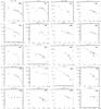 |
Fig. 3 Radio spectra of the 25 BAL and 34 non-BAL QSOs (GHz on x-axis, mJy on y-axis). Error bars are shown when larger than the symbol size. Crosses represent flux densities from the literature, rhombi are flux densities from our observational campaign, and arrows are upper limits from the literature. Solid lines are fits to a parabola and dashed lines are fits to a power law. For resolved sources, flux densities are presented as follows: a square for C component (core) and triangle, asterisk, and dot for components A, B, and D, respectively (see Tables 5 and 6). For 1728+56, the flux densities at 4.8 and 8.4 GHz shown as asterisks correspond to the B+C components. |
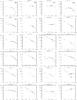 |
Fig. 3 continued. |
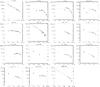 |
Fig. 3 continued. |
The measured flux densities (in mJy) for the sample of 25 radio-loud BAL QSOs.
Flux densities for the sample of 34 non-BAL QSOs (see the caption of Table 5 for details).
Low-frequency flux densities (in mJy) from the literature (see Sect. 4 for references) for the samples of BAL (upper list) and non-BAL (bottom list) QSOs.
Radio spectral shape and spectral indices of the QSO sample.
The populations of radio-loud and radio-quiet QSOs correspond to radio luminosities of L5 GHz ≥ 1026 W Hz-1 and L5 GHz < 1025 W Hz-1, respectively (Miller et al. 1990).
Acknowledgments
We are grateful to F. Mantovani for helping us during the observations at the 100-m Effelsberg telescope. We would also like to thank A. Mignano, from the ALMA Regional Centre (Italian node), for helping us in image analysis with the first release of the CASA astronomical software. Part of this work was supported by a grant of the Italian Programme for Research of Relevant National Interest (PRIN No. 18/2007, PI: K.-H. Mack) The authors acknowledge financial support from the Spanish Ministerio de Ciencia e Innovación under project AYA2008-06311-C02-02. This work has benefited from research funding from the European Union’s sixth framework programme under RadioNet grant agreement No. 227290. This work has been partially based on observations with the 100-m telescope of the MPIfR (Max-Planck-Institut für Radioastronomie) at Effelsberg. The National Radio Astronomy Observatory is a facility of the National Science Foundation operated under cooperative agreement by Associated Universities, Inc. This research has made use of the NASA/IPAC Infrared Science Archive and NASA/IPAC Extragalactic Database (NED) which are both operated by the Jet Propulsion Laboratory, California Institute of Technology, under contract with the National Aeronautics and Space Administration. Use has been made of the Sloan Digital Sky Survey (SDSS)
Archive. The SDSS is managed by the Astrophysical Research Consortium (ARC) for the participating institutions: The University of Chicago, Fermilab, the Institute for Advanced Study, the Japan Participation Group, The John Hopkins University, Los Alamos National Laboratory, the Max-Planck-Institute for Astronomy (MPIA), the Max-Planck-Institute for Astrophysics (MPA), New Mexico State University, University of Pittsburgh, Princeton University, the United States Naval Observatory, and the University of Washington.
References
- Adelman-McCarthy, J. K., Agüeros, M. A., Allam, S. S., et al. 2007, ApJS, 172, 634 [NASA ADS] [CrossRef] [Google Scholar]
- Baars, J. W. M., Genzel, R., Pauliny-Toth, I. I. K., et al. 1977, A&A, 61, 99 [NASA ADS] [Google Scholar]
- Barvainis, R., Lehár, J., Birkinshaw, M., et al. 2005, ApJ, 618, 108 [NASA ADS] [CrossRef] [Google Scholar]
- Becker, R. H., White, R. L., & Helfand, D. J. 1995, ApJ, 450, 559 [NASA ADS] [CrossRef] [Google Scholar]
- Becker, R. H., White, R. L., Gregg, M. D., et al. 2000, ApJ, 538, 72 [NASA ADS] [CrossRef] [Google Scholar]
- Becker, R. H., White, R. L., Gregg, M. D., et al. 2001, ApJS, 135, 227 [NASA ADS] [CrossRef] [Google Scholar]
- Benn, C. R., Carballo, R., Holt, J., et al. 2005, MNRAS, 360, 1455 [NASA ADS] [CrossRef] [Google Scholar]
- Briggs, F. H., Turnsheck, D. A., & Wolfe, M. 1984, ApJ, 287, 549 [NASA ADS] [CrossRef] [Google Scholar]
- Cohen, A. S., Lane, W. M., Cotton, W. D., et al. 2007, AJ, 134, 1245 [NASA ADS] [CrossRef] [Google Scholar]
- Condon, J. J., Cotton, W. D., Greisen, E. W., et al. 1998, AJ, 115, 1693 [NASA ADS] [CrossRef] [Google Scholar]
- Dallacasa, D., Stanghellini, C., Centoza, M., et al. 2000, A&A, 363, 887 [NASA ADS] [Google Scholar]
- de Bruyn, G., Miley, G., Rengelink, R., et al. 2000, VizieR On-line Data Catalog VIII/62 [Google Scholar]
- Douglas, J. N., Bash, F. N., & Bozyan, F. A. 1996, AJ, 111, 1945 [NASA ADS] [CrossRef] [Google Scholar]
- Elvis, M. 2000, ApJ, 545, 63 [NASA ADS] [CrossRef] [Google Scholar]
- Fanti, R., Fanti, C., Schilizzi, R. T., et al. 1990, A&A, 231, 333 [NASA ADS] [Google Scholar]
- Feigelson, E. D., & Nelson, P. I. 1985, ApJ, 293, 192 [NASA ADS] [CrossRef] [Google Scholar]
- Ficarra, A., Grueff, G., & Tomasetti, G. 1984, A&AS, 59, 255 [Google Scholar]
- Ghosh, K. K., & Punsly, B. 2007, ApJ, 661, 139 [Google Scholar]
- Gupta, N., Salter, C. J., Saikia, D. J., Ghosh, T., & Jeyakumar, S. 2006, MNRAS, 373, 972 [NASA ADS] [CrossRef] [Google Scholar]
- Hewett, P. C., & Foltz, C. B. 2003, AJ, 125, 1784 [NASA ADS] [CrossRef] [Google Scholar]
- Hales, S. E. G., Baldwin, J. E., & Warner, P. J. 1988, MNRAS, 234, 919 [Google Scholar]
- Hall, P. B., Anderson, S. F., Strauss, M. A., et al. 2002, ApJS, 141, 267 [NASA ADS] [CrossRef] [Google Scholar]
- Kato, T., Tabara, H., Inoue, M., et al. 1987, Nature, 329, 223 [NASA ADS] [CrossRef] [Google Scholar]
- Klein, U., Mack, K.-H., Gregorini, L., et al. 2003, A&A, 406, 579 [NASA ADS] [CrossRef] [EDP Sciences] [Google Scholar]
- Kovalev, Y. Y. 1996, in Extragalactic radio sources, ed. R. D. Ekers, C. Fanti, & L. Padrielli (Dordrecht: Kluwer), IAU Symp., 175, 95 [Google Scholar]
- Lípari, S. L., & Terlevich, R. J. 2006, MNRAS, 368, 1011 [Google Scholar]
- Miller, L., Peacock, J. A., & Mead, A. R. G. 1990, MNRAS, 244, 207 [NASA ADS] [Google Scholar]
- Montenegro-Montes, F. M., Mack, K.-H., Vigotti, M., et al. 2008a, MNRAS, 388, 1853 (MM08) [NASA ADS] [CrossRef] [Google Scholar]
- Montenegro-Montes, F. M., Mack, K.-H., Benn, C., et al. 2008b, PoS (IX EVN Symposium) 019 [Google Scholar]
- Morganti, R. 2008, in Extragalactic Jets: Theory and Observation from Radio to Gamma Ray, ed. T. A. Rector, & D. S. De Young, Girdwood, Alaska, ASP Conf. Ser., 386, 210 [Google Scholar]
- O’Dea, C. P. 1998, PASP, 110, 493 [NASA ADS] [CrossRef] [Google Scholar]
- O’Dea, C. P., & Baum, S. A. 1997, AJ, 113, 148 [NASA ADS] [CrossRef] [Google Scholar]
- Orr, M. J. L., & Browne, I. W. A. 1982, MNRAS, 200, 1067 [NASA ADS] [CrossRef] [Google Scholar]
- Punsly, B. 1999a, ApJ, 527, 609 [NASA ADS] [CrossRef] [Google Scholar]
- Punsly, B. 1999b, ApJ, 527, 624 [NASA ADS] [CrossRef] [Google Scholar]
- Pollack, L. K., Taylor, G. B., & Zavala, R. T. 2003, ApJ, 589, 733 [NASA ADS] [CrossRef] [Google Scholar]
- Sadler, E. M., Ricci, R., Ekers, R. D., et al. 2006, MNRAS, 371, 898 [NASA ADS] [CrossRef] [Google Scholar]
- Schneider, D. P., Hall, P. B., Richards, G. T., et al. 2007, AJ, 134, 102 [NASA ADS] [CrossRef] [Google Scholar]
- Stocke, J. T., Morris, S. L., Weymann, R. J., et al. 1992, ApJ, 396, 487 [NASA ADS] [CrossRef] [Google Scholar]
- Taylor, A. R., Stil, J. M., & Sunstrum, C. 2009, ApJ, 702, 1230 [NASA ADS] [CrossRef] [Google Scholar]
- Torniainen, H., Tornikoski, M., Terasranta, H., et al. 2005, A&A, 435, 839 [NASA ADS] [CrossRef] [EDP Sciences] [Google Scholar]
- Trump, J. R., Hall, P. B., Reichard, T. A., et al. 2006, ApJS, 165, 1 [NASA ADS] [CrossRef] [Google Scholar]
- van Breugel, W., Miley, G., & Heckman, T. 1984, AJ, 89, 5 [NASA ADS] [CrossRef] [Google Scholar]
- Vigotti, M., Grueff, G., Perley, R., et al. 1989, AJ, 98, 419 [NASA ADS] [CrossRef] [Google Scholar]
- Vigotti, M., Vettolani, G., Merighi, R., et al. 1997, A&AS, 123, 219 [NASA ADS] [CrossRef] [EDP Sciences] [Google Scholar]
- Vigotti, M., Gregorini, L., Klein, U., et al. 1999, VizieR On-line Data Catalog: J/A+AS/139/359 [Google Scholar]
- Weymann, R. J., Morris, S. L., Foltz, C. B., et al. 1991, ApJ, 373, 23 [NASA ADS] [CrossRef] [Google Scholar]
- White, R. L., Becker, R. H., Gregg, M. D., et al. 1997, A&AS, 29, 1373 [Google Scholar]
- Zavala, R. T., & Taylor, G. B. 2004, ApJ, 612, 749 [NASA ADS] [CrossRef] [Google Scholar]
- Zhou, H., Wang, T., Wang, H., et al. 2006, ApJ, 639, 716 [NASA ADS] [CrossRef] [Google Scholar]
All Tables
Sources with significant variability, σVar > 4, from the observations in this paper.
Fractional polarisation m (in percentage), at several frequencies (ν in GHz), for the BAL QSO sample.
Flux densities for the sample of 34 non-BAL QSOs (see the caption of Table 5 for details).
Low-frequency flux densities (in mJy) from the literature (see Sect. 4 for references) for the samples of BAL (upper list) and non-BAL (bottom list) QSOs.
All Figures
|
Fig. 1 Distribution in flux density and redshift, of the QSOs in both the BAL (crosses) and non-BAL (circles) samples. |
| In the text | |
|
Fig. 2 Maps of the resolved QSOs. The synthesised beam size is shown in the lower left corner of the map. Levels are multiples of the 3-σ flux density value in mJy/beam, according to the legend. A cross indicates the SDSS optical position. |
| In the text | |
|
Fig. 2 continued. |
| In the text | |
|
Fig. 4
|
| In the text | |
|
Fig. 5 Distribution of the radio spectral indices ( |
| In the text | |
|
Fig. 6 Cumulative distribution of the fractional polarisation for the two samples, at each of three frequencies. Each pair of numbers in parenthesis indicates the number of detections and the number of upper limits at that frequency. The dashed lines indicate the 50% percentile (i.e. the median) and the 85% percentile. |
| In the text | |
|
Fig. 7 Linear fits of the polarisation angles χ versus the square of the observed wavelengths for 4 BAL QSOs and 10 non-BAL QSOs, yielding the rotation measures. The errors in the position angles are lower than the dot size. Triangles correspond to the polarisation percentages (m). |
| In the text | |
|
Fig. 3 Radio spectra of the 25 BAL and 34 non-BAL QSOs (GHz on x-axis, mJy on y-axis). Error bars are shown when larger than the symbol size. Crosses represent flux densities from the literature, rhombi are flux densities from our observational campaign, and arrows are upper limits from the literature. Solid lines are fits to a parabola and dashed lines are fits to a power law. For resolved sources, flux densities are presented as follows: a square for C component (core) and triangle, asterisk, and dot for components A, B, and D, respectively (see Tables 5 and 6). For 1728+56, the flux densities at 4.8 and 8.4 GHz shown as asterisks correspond to the B+C components. |
| In the text | |
|
Fig. 3 continued. |
| In the text | |
|
Fig. 3 continued. |
| In the text | |
Current usage metrics show cumulative count of Article Views (full-text article views including HTML views, PDF and ePub downloads, according to the available data) and Abstracts Views on Vision4Press platform.
Data correspond to usage on the plateform after 2015. The current usage metrics is available 48-96 hours after online publication and is updated daily on week days.
Initial download of the metrics may take a while.