| Issue |
A&A
Volume 542, June 2012
GREAT: early science results
|
|
|---|---|---|
| Article Number | L17 | |
| Number of page(s) | 4 | |
| Section | Letters | |
| DOI | https://doi.org/10.1051/0004-6361/201218923 | |
| Published online | 10 May 2012 | |
The structure of hot gas in Cepheus B
1 Department of Astronomy and Astrophysics, Tata Institute of Fundamental Research, Homi Bhabha Road, Colaba, 400005 Mumbai, India
e-mail: This email address is being protected from spambots. You need JavaScript enabled to view it.
2 KOSMA, I. Physikalisches Institut, Universität zu Köln, Zülpicher Str. 77, 50937 Köln, Germany
3 Max-Planck-Institut für Radioastronomie, Auf dem Hügel 69, 53121 Bonn, Germany
4 Instituto de Radio Astronomía Milimétrica (IRAM), Avenida Divina Pastora 7, Local 20, 18012 Granada, Spain
Received: 31 January 2012
Accepted: 24 February 2012
Abstract
By observing radiation-affected gas in the Cepheus B molecular cloud, we probe whether the sequential star formation in this source is triggered by the radiation from newly formed stars. We used the dual band receiver GREAT onboard SOFIA to map [C ii] and CO 13–12 and 11–10 in Cep B and compared the spatial distribution and the spectral profiles with complementary ground-based data of low-J transitions of CO isotopes, atomic carbon, and the radio continuum. The interaction of the radiation from the neighboring OB association creates a large photon-dominated region (PDR) at the surface of the molecular cloud traced through the photoevaporation of C+. Bright internal PDRs of hot gas are created around the embedded young stars, where we detect evidence of the compression of material and local velocity changes; however, on the global scale we find no indications that the dense molecular material is dynamically affected.
Key words: ISM: clouds / ISM: individual objects: Cep B / ISM: kinematics and dynamics / ISM: molecules / radio lines: ISM / photon-dominated region (PDR)
© ESO, 2012
1. Introduction
The molecular cloud Cepheus B, located at a distance of about 730 pc can be regarded as a prototype of a region with sequential star formation. It has a wedge-like shape, pointing NW to the young Cepheus OB3 association, including the luminous stars HD 217086 (O7) and HD 217061 (B1). The OB association is composed of two subgroups of different ages, where the youngest group lies closer to the molecular cloud (Sargent 1977). The radiation from the association creates a brightH ii region, S155, at the cloud surface. Deeper in the cloud, star formation continues (Moreno-Corral et al. 1993), creating a hot core (Felli et al. 1978) that was resolved into two ultracompact and one extended H ii regions by Testi et al. (1995). The main energy source in the hot core is a B1 star in source A of Testi et al. (1995), but more pre-main-sequence stars are contained in the hot core (Moreno-Corral et al. 1993). The density of molecular material increases further towards the SE, where two neighboring column density peaks have been identified through observations of low-J13CO and C18O (Ungerechts et al. 2000; Mookerjea et al. 2006). The molecular cloud observations by Beuther et al. (2000) showed a clumpy structure that allows a deep penetration of UV radiation from the OB association and a large-scale velocity gradient with blueshifted velocities towards the OB association. At a resolution of 43′′, three [C ii] spectra at 158 μ were observed in Cepheus B using the KAO (Boreiko et al. 1990). The [C ii] spectra was found to have two velocity components, one associated with the molecular material and one with S155. The CO 4–3 and [C i] observations of Mookerjea et al. (2006) showed that the main heating of the molecular material occurs in PDRs (photon-dominated regions) created below S 155 and around the hot-spot H ii regions. The FUV field is estimated to be between 1500 to 25χ0, where χ0 is the average interstellar radiation field (Draine 1978).
To look for indications of sequential star formation due to radiative triggering as proposed by Getman et al. (2009), the density, temperature structure, and kinematics of the FUV irradiated PDRs at the cloud surfaces need to be probed. Signs of triggering processes would be the formation of density enhancements correlated with the radiative pressure increase at the cloud surface (radiative shells, see e.g. Dale et al. 2009) or indications of velocity gradients in the molecular material created below the radiative compression zones.
To address these questions, we performed spectral mapping observations of Cep B in [C ii] and CO 13–12 and 11–10 using the German REceiver for Astronomy at Terahertz frequencies (GREAT1, Heyminck et al. 2012) onboard the Stratospheric Observatory For Infrared Astronomy (SOFIA). The new data were combined with existing observations of low-J CO isotopologs and [C i] to probe the structure of the PDR and the velocity distribution.
2. Observations
We observed the hot core region of Cepheus B during the nights of April 7 and July 19, 2011 with GREAT on SOFIA at an altitude of ~42 000 feet. During the two nights were observed areas of the same size (2 4 × 16), but offset relative to each other. GREAT is a modular heterodyne instrument, with two channels used simultaneously. In April, channel L1#a was tuned to CO 11–10 (1267.015 GHz), and channel L2 was tuned to [C ii] 2P3/2 → 2P1/2 (1900.537 GHz) for four coverages of the region. In July, L1#b was tuned to CO 13–12 (1496.923 GHz), while L2 was tuned to [C ii] for three coverages. The HPBWs are 21
 3 at 1.3 THz, 196 at 1.5 THz, and 15′′ at 1.9 THz.
The observations were performed in position-switched on-the-fly (OTF) mode with an OFF position at Δα = −600″;Δδ = + 600″. As backend we used the acousto optic spectrometer with a bandwidth of 1 GHz and a resolution of 1.6 MHz. The integration time was 0.6 min/position. The measured system temperatures were 3100 K for CO 11–10, 2500 K for CO 13–12, and 3200–3500 K for [C ii]. The forward efficiency is ηf = 0.95, and the main beam efficiencies (ηmb) are 0.51 for [C ii] and 0.53 for CO 11–10 lines (Guan et al. 2012). Details of calibration of the data are presented by Guan et al. (2012). We fitted and subtracted baselines of the fourth or sixth order to the [C ii] and CO data.
Complementary observations of [C i] (3P1 → 3P0 at 492.161 GHz) were performed in December 2002 using the CHAMP 2 × 8 pixel array receiver (Güsten et al. 1998) at the CSO. The fully sampled [C i] map of 33 × 37 was observed in position-switched mode (reference position − 300′′, 0). The HPBW for [C i] was 145 at 492 GHz and ηMB was 0.51 (Philipp et al. 2006). The [C i] data were smoothed to 20′′ for comparison.
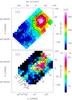 |
Fig. 1 a) Velocity-integrated intensity map of [C ii] in color and contors. The contor levels are at 79 to 339.4 K km s-1 (peak) in steps of 29 K km s-1. b) Integrated intensity map of CO 11–10 (color) overlayed with contors of CO 13–12 (white) and [C ii] (black) intensities. Contour levels for CO 13–12 are: 2.1 to 11.7 K km s-1 (peak). vLSR-range of integration is [C ii]: [ − 20; − 5], CO: [ − 16; − 11] km s-1. The white star denotes the B1 star at (α;δ) = (22h57m6.2s;62°37′55.4″). Offsets of the marked CO peaks #1, #2, and #3 are ( − 45′′, +64′′), ( − 41′′, +20′′), and ( − 9′′, +3′′), respectively. |
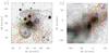 |
Fig. 2 a) Optical image (grayscale) overlayed with contors of 8.4 GHz continuum emission (black) (Testi et al. 1995) and contors of [C ii] (green dashed) and CO 11–10 (red). b) Intensity of 13CO 2–1 emission integrated between vLSR = −17 to − 10 km s-1 (Ungerechts et al. 2000) (grayscale) overlayed with contors of CO 11–10 (red) and [C ii] (green dotted). Contour levels of [C ii] are the same as inFig. 1, for CO 11–10: 6.8 to 32.1 K km s-1 (peak) in steps of 3.6 K km s-1. The star and the triangle denote the positions of Testi’s NIR sources A and B, respectively. |
3. Morphology
Figure 1 shows the integrated intensity maps of [C ii] and CO 11–10 and CO 13–12. The (0, 0) position of the maps is at  and δ = 62°34′23″ (J2000). The [C ii] emission shows a single peak (
 ,
,  ) located to the W of an embedded B1 star, and the emission drops towards the E. The CO 11–10 exhibits three peaks referred to as #1, #2, and #3 in the rest of the paper, forming a shell around the [C ii] peak. The emission is extended further in the NW-SE direction.
Figure 2a compares the [C ii] and CO 11–10 observations with radio continuum observations by Testi et al. (1995). Testi et al. show that the 8.4 GHz radio continuum emission component A, a blister H ii region, peaks slightly to the SW of the position of the B1 star. We find a sequence of peaks in that direction starting with the radio continuum close to the heating star, the [C ii] peak, and the CO 11–10 peak #2, consistent with the expected layered structure of a PDR. The CO 11–10 peaks #2 and #3, both S of the source A trace dense and warm molecular gas. Peak #1 coincides with the radio source B (Testi et al. 1995). The CO 13–12 emission appears to be centered close to the B1 star, but the detailed distribution around it could not be observed due to time constraints.
Figure 2b compares our data with IRAM 30m 13CO 2–1 observations at 10′′ resolution by Ungerechts et al. (2000), tracing molecular gas with high column densities, which has a ridge like structure extended towards the main cloud E of the map. A similar intensity distribution is also seen in the 13CO 1–0 map (Ungerechts et al. 2000), the [C i] 1–0 map (see Fig. 3), and in the CO 4–3 map (at 1′Mookerjea et al. 2006). The CO 11–10 peak #3 coincides with a column density peak in these maps, while peaks #1 and #2 indicate an increased CO excitation, e.g. due to a higher temperature of the molecular material. More PDR layers are formed at the surface of the molecular material in the SE. They are also traced by the [C ii] and the high-J CO lines but at a low level of emission. We detect almost no CO emission to the N and NE of the embedded B1 star.
Since [C ii] can also originate in ionized gas, it is reasonable to expect enhanced [C ii] emission at the location of the radio continuum peaks detected by Testi et al. (1995). However, the [C ii] emission shows no enhancement at the location of the CO peak #1, which coincides with the B-component. This indicates that the source creating the B-component of the radio continuum emission ionizes at most a small fraction of the molecular material, consistent with Testi’s suggestion that source B is a protostar, not yet ionizing, but heating up its surroundings.
Our observations are consistent with Testi’s suggestion of a blister-type H ii-region for component A, created by the B1 star, and a density gradient of the surrounding material leading to an “open cone” configuration. The density decreases to the N, so the cone opens in this direction. The ionized material may escape to the N, but cannot expand much to the S because of denser molecular material there. This results in increased and sharply bounded radio continuum emission to the S and in extended, but lower intensity emission to the N of the position of the embedded star.
4. PDR layering
As discussed above we find a layering sequence of [C ii], high-J CO and low-J CO peaks around the H ii region associated with the B1 star. Figure 3 shows the effect of this layering in terms of the mutual shift of the peaks of the [C ii], CO 11–10, and 13CO 2–1 emission. We find a separation of about 0.02 pc between [C ii] and CO 11–10 and of 0.08 pc between [C ii] and 13CO 2–1. For [C i] the peak emission is seen at the edge of the mapped region. The [C i] distribution is similar to that of 13CO 2–1, but the emission is weak in the considered cut. The shift in the peaks is consistent with the predictions of a uniform PDR model, although in reality, it will also be affected by small-scale density variations.
For a qualitative comparison we used the KOSMA-τ PDR model (Röllig et al. 2006) to simulate gas temperature and chemical structure inside the PDR. KOSMA-τ considers a spherical clump illuminated by an isotropic FUV radiation field and cosmic rays. Input parameters are the radiation field, the clump mass and the density at the clump surface. It assumes that the clump has a power-law density profile of n(r) ∝ r-1.5 for 0.2 ≤ r/rcl ≤ 1 and n(r) = const. for r/rcl ≤ 0.2. To simulate a plane-parallel PDR through a spherical model, we chose a clump of 103 M⊙, i.e. with a mass much larger than the available molecular mass (see Mookerjea et al. 2006). The outer layers of this massive clump then form an almost plane-parallel configuration suitable to studying the observed stratification.
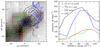 |
Fig. 3 Left: map of integrated intensity distributions of 13CO 2–1 (greyscale, red contor), [C ii] (black), CO 11–10 (blue), and [C i] (green). Right: cut through the [C ii] peak and the CO 11–10 peak #2. The black dotted vertical line denotes the position closest to the B1 star along the cut. Integration ranges: [C ii] and [C i] [ − 20; − 5], CO 11–10, and 13CO [ − 17; − 10] ( km s-1). |
Figure 4 shows the local optically thin emissivity, i.e. the intensities per cloud depth without optical depth correction, for two models with a density n(rcl = 105 cm-3 and n(rcl = 106 cm-3 illuminated by a radiation field of 1000 χ0 (Mookerjea et al. 2006). The model predicts a stratification with a 0.001...0.01 pc separation of the CO 11–10 peak relative to the [C ii] peak and a further separation of 0.12...0.3 pc to the 13CO 2–1 peak2, indicating that the parameters used are reasonable, but do not provide a full match to the observations. The observed intensity ratios of the three lines suggest that the density in the cloud is closer to 106 cm-3 than to 105 cm-3. Since the CO 11–10 line is very sensitive to the gas density, the similar peak intensities at #2 and #3 indicate approximately equal gas densities, while the higher 13CO and [C i] intensities at peak #3 indicate higher column densities of molecular gas there.
The model, however, predicts a narrow, but weak [C i] peak in front of the CO 11–10 layer, while the [C i] emission is very extended on the map3. In contradiction to the model, the [C i] emission seems to measure the molecular column density, so not following the stratification of the other tracers.
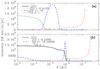 |
Fig. 4 Optically thin line intensities per cloud depth for the two model densities: a) nsurf = 106 cm-3, b) nsurf = 105 cm-3. Radiation field and clump mass are 1000 χ0 and 1000 M⊙, respectively. |
5. Velocity structure
To study the main characteristics of the [C ii] velocity distribution we show inFig. 5 the map of the centroid velocities and the corresponding position-velocity diagram for a cut through the map. The map of the centroid velocities was generated by fitting a single-component Gaussian profile to each spectrum. The velocity distribution is dominated by a large-scale gradient of about 1 km s-1 over 200′′ from NW to SE, visible as a color gradient inFig. 5a and as a global slope inFig. 5b. This is consistent with the velocity gradient of 4.2 × 10⁻³ km s-1/arcsec in the molecular cloud derived from the channel maps of CO 3–2 observations (Beuther et al. 2000). Moreover, one can see a good correlation between the centroid velocity map and the 13CO map inFig. 2 in the sense that pixels associated with strong emission in low- and mid-J CO have systematically higher velocities than nearby pixels measuring lower density material. The velocity of the low-density material is closer to that of S155; i.e., the ionized gas is always somewhat blueshifted relative to the denser molecular cloud.
The position-velocity diagram ( Fig. 5b) shows a broadening of the [C ii] line at the position of the [C ii] peak and there appears to be an additional velocity component visible as a blue shoulder. An interesting feature is, however, the change in the velocity gradient around the [C ii] peak. The contors in the PV diagram form a parallelogram NW of the peak where the large-scale velocity gradient is inverted. The inversion is not very pronounced when considering the Gauss-fit velocities along the cut, but is apparent as higher velocity in the map ( Fig. 5a) around CO peak #2.
To look at the details of the spectral profiles, we averaged the spectra around the peak positions #1, #2, and #3 over an area of 33′′ diameter ( Fig. 6). We find emission from different velocity components. The normal molecular cloud material at velocities of −13.5... −13 km s-1 is traced by 13CO 2–1, [C i], and CO 11–10 in #1 and #3. In this complementary analysis approach, involving positions not all on the cut discussed above, we find that at #2, CO 11–10 is, significantly blueshifted, showing a local inversion of the velocity gradient similar to the inversion seen in [C ii] along the cut. This means that the embedded B1 star not only creates a localH ii region, but it also affects the dynamics of the hot gas in the PDR around theH ii region on a scale of about 30′′, i.e. 0.1 pc.
The [C ii] line is much wider at all positions. It includes the velocity of the molecular cloud but also an additional blueshifted component with velocities of about −16 km s-1 and a wing extending down to −21 km s-1. Boreiko et al. (1990) showed that the −16 km s-1 component matches the vLSR of the Hα emission from the H ii region S155. At #1, this −16 km s-1 is the dominant component, showing that most of the [C ii] emission stems from theH ii region there. The broad blue wing is, however, also present at #2 and #3, and actually strongest at #3. This may represent ionized material that is ablating from the cloud surface. Depending on the exact geometry of cloud and main radiation source, we find two possible interpretations. If HD 217086, located slightly behind the cloud (Felli et al. 1978), represents the main sources of UV photons, the acceleration of low-density material through the radiation pressure could lead to the wing of blueshifted material. If HD 217061, in front of the cloud, is the main radiation source, we could be tracing the signature of a photoevaporation flow from the surface as predicted by Gorti & Hollenbach (2002). Detailed analysis confirming either of the two possibilities is beyond the scope of this paper.
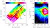 |
Fig. 5 a) Map of the vLSR values (inkm s-1) for Gaussian fits to the [C ii] spectra. b) PV diagram for [C ii] along the cut indicated in a). The white line shows the position of the [C ii] peak and the solid black line the centroid velocity along the cut. |
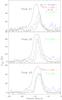 |
Fig. 6 Spectra averaged over an area of 33′′ diameter around the CO 11–10 peaks #1, #2, and #3. |
6. Conclusion
The [C ii] emission is affected on large scales by radiation from the Cepheus OB3 association with a gradual change from material stemming mostly from the S155H ii region in the NW through material photoevaporating from the molecular cloud surface, which is potentially accelerated by radiation pressure, to PDR material within the molecular cloud that is ionized through the FUV radiation, but resides at the velocities of the parental cloud with the known large-scale velocity gradient. For the tracers of the denser material, we find no large-scale effects but local velocity shifts due to the embedded ultracompactH ii regions. They create a partially inverted velocity gradient, a local broadening of the line profiles and disperses the material around them, but do not create any long-range effects.
Overall, we found no indications that a radiative triggering mechanism creates the sequential star formation in Cepheus B. Radiative star-formation triggering may work on very small scales around theH ii regions mostly unresolved here, but cannot explain a large-scale sequence.
GREAT is a development by the MPI für Radioastronomie and KOSMA/Universität zu Köln, in cooperation with the MPI für Sonnensystemforschung and the DLR Institut für Planetenforschung.
13CO 2–1 always shows a broad peak filling a large fraction of the clump core, independent of the clump mass, indicating that the displacement of the 13CO 2–1 peak relative to the PDR surface is fairly well determined by the density structure than by illumination.
Spot checks with the PDR models by M. Kaufman and the Meudon group show the same inversion in the [C i] layering that we find with the KOSMA-τ model.
Acknowledgments
We thank Sabine Philipp for providing us with the CHAMP [C i] data and Hans Ungerechts for providing the IRAM 13CO data. This paper is based on observations made with the NASA/DLR Stratospheric Observatory for Infrared Astronomy. SOFIA Science Mission Operations are conducted jointly by the Universities Space Research Association, Inc., under NASA contract NAS2-97001, and the Deutsches SOFIA Institut under DLR contract 50 OK 0901. We thank the SOFIA engineering and operations teams for their support during Early Science. The research presented here was supported by the German Deutsche Forschungsgemeinschaft, DFG through project number SFB 956C. This research made use of the SIMBAD database, operated at the CDS, Strasbourg, France, and NASA’s Astrophysics Data System Bibliographic Services.
References
- Beuther, H., Kramer, C., Deiss, B., & Stutzki, J. 2000, A&A, 362, 1109 [Google Scholar]
- Boreiko, R. T., Betz, A. L., & Zmuidzinas, J. 1990, ApJ, 353, 181 [NASA ADS] [CrossRef] [PubMed] [Google Scholar]
- Dale, J. E., Wünsch, R., Whitworth, A., & Palouš, J. 2009, MNRAS, 398, 1537 [NASA ADS] [CrossRef] [Google Scholar]
- Draine, B. T. 1978, ApJS, 36, 595 [NASA ADS] [CrossRef] [Google Scholar]
- Felli, M., Tofani, G., Harten, R. H., & Panagia, N. 1978, A&A, 69, 199 [NASA ADS] [Google Scholar]
- Getman, K. V., Feigelson, E. D., Luhman, K. L., et al. 2009, ApJ, 699, 1454 [NASA ADS] [CrossRef] [Google Scholar]
- Gorti, U., & Hollenbach, D. 2002, ApJ, 573, 215 [NASA ADS] [CrossRef] [Google Scholar]
- Guan, X., Stutzki, J., Graf, U. U., et al. 2012, A&A, 542, L4 [Google Scholar]
- Güsten, R., Ediss, G. A., Gueth, F., et al. 1998, Proc. SPIE, 3357, 167 [NASA ADS] [CrossRef] [Google Scholar]
- Heyminck, S., Graf, U. U., Güsten, R., et al. 2012, A&A, 542, L1 [NASA ADS] [CrossRef] [EDP Sciences] [Google Scholar]
- Mookerjea, B., Kramer, C., Röllig, M., & Masur, M. 2006, A&A, 456, 235 [NASA ADS] [CrossRef] [EDP Sciences] [Google Scholar]
- Moreno-Corral, M. A., Chavarria, K. C., de Lara, E., et al. 1993, A&A, 273, 619 [NASA ADS] [Google Scholar]
- Philipp, S. D., Lis, D. C., Güsten, R., et al. 2006, A&A, 454, 213 [NASA ADS] [CrossRef] [EDP Sciences] [Google Scholar]
- Röllig, M., Ossenkopf, V., Jeyakumar, S., et al. 2006, A&A, 451, 917 [NASA ADS] [CrossRef] [EDP Sciences] [Google Scholar]
- Sargent, A. I. 1977, ApJ, 218, 736 [NASA ADS] [CrossRef] [Google Scholar]
- Testi, L., Olmi, L., Hunt, L., et al. 1995, A&A, 303, 881 [NASA ADS] [Google Scholar]
- Ungerechts, H., Brunswig, W., Kramer, C., et al. 2000, Imaging at Radio through Submillimeter Wavelengths, ed. J. G. Mangum, & S. J. E. Radford, ASP Conf. Proc., 217, 190 [Google Scholar]
All Figures
|
Fig. 1 a) Velocity-integrated intensity map of [C ii] in color and contors. The contor levels are at 79 to 339.4 K km s-1 (peak) in steps of 29 K km s-1. b) Integrated intensity map of CO 11–10 (color) overlayed with contors of CO 13–12 (white) and [C ii] (black) intensities. Contour levels for CO 13–12 are: 2.1 to 11.7 K km s-1 (peak). vLSR-range of integration is [C ii]: [ − 20; − 5], CO: [ − 16; − 11] km s-1. The white star denotes the B1 star at (α;δ) = (22h57m6.2s;62°37′55.4″). Offsets of the marked CO peaks #1, #2, and #3 are ( − 45′′, +64′′), ( − 41′′, +20′′), and ( − 9′′, +3′′), respectively. |
| In the text | |
|
Fig. 2 a) Optical image (grayscale) overlayed with contors of 8.4 GHz continuum emission (black) (Testi et al. 1995) and contors of [C ii] (green dashed) and CO 11–10 (red). b) Intensity of 13CO 2–1 emission integrated between vLSR = −17 to − 10 km s-1 (Ungerechts et al. 2000) (grayscale) overlayed with contors of CO 11–10 (red) and [C ii] (green dotted). Contour levels of [C ii] are the same as inFig. 1, for CO 11–10: 6.8 to 32.1 K km s-1 (peak) in steps of 3.6 K km s-1. The star and the triangle denote the positions of Testi’s NIR sources A and B, respectively. |
| In the text | |
|
Fig. 3 Left: map of integrated intensity distributions of 13CO 2–1 (greyscale, red contor), [C ii] (black), CO 11–10 (blue), and [C i] (green). Right: cut through the [C ii] peak and the CO 11–10 peak #2. The black dotted vertical line denotes the position closest to the B1 star along the cut. Integration ranges: [C ii] and [C i] [ − 20; − 5], CO 11–10, and 13CO [ − 17; − 10] ( km s-1). |
| In the text | |
|
Fig. 4 Optically thin line intensities per cloud depth for the two model densities: a) nsurf = 106 cm-3, b) nsurf = 105 cm-3. Radiation field and clump mass are 1000 χ0 and 1000 M⊙, respectively. |
| In the text | |
|
Fig. 5 a) Map of the vLSR values (inkm s-1) for Gaussian fits to the [C ii] spectra. b) PV diagram for [C ii] along the cut indicated in a). The white line shows the position of the [C ii] peak and the solid black line the centroid velocity along the cut. |
| In the text | |
|
Fig. 6 Spectra averaged over an area of 33′′ diameter around the CO 11–10 peaks #1, #2, and #3. |
| In the text | |
Current usage metrics show cumulative count of Article Views (full-text article views including HTML views, PDF and ePub downloads, according to the available data) and Abstracts Views on Vision4Press platform.
Data correspond to usage on the plateform after 2015. The current usage metrics is available 48-96 hours after online publication and is updated daily on week days.
Initial download of the metrics may take a while.