| Issue |
A&A
Volume 542, June 2012
|
|
|---|---|---|
| Article Number | A48 | |
| Number of page(s) | 26 | |
| Section | Catalogs and data | |
| DOI | https://doi.org/10.1051/0004-6361/201218829 | |
| Published online | 04 June 2012 | |
The AMBRE Project: Stellar parameterisation of the ESO:FEROS archived spectra
Laboratoire Lagrange (UMR7293), Université de Nice Sophia Antipolis, CNRS, Observatoire de la Côte d’Azur, BP 4229, 06304 Nice Cedex 4, France
e-mail: This email address is being protected from spambots. You need JavaScript enabled to view it.
Received: 17 January 2012
Accepted: 20 March 2012
Abstract
Context. The AMBRE Project is a collaboration between the European Southern Observatory (ESO) and the Observatoire de la Côte d’Azur (OCA) that has been established in order to carry out the determination of stellar atmospheric parameters for the archived spectra of four ESO spectrographs.
Aims. The analysis of the FEROS archived spectra for their stellar parameters (effective temperatures, surface gravities, global metallicities, alpha element to iron ratios and radial velocities) has been completed in the first phase of the AMBRE Project. From the complete ESO:FEROS archive dataset that was received, a total of 21 551 scientific spectra have been identified, covering the period 2005 to 2010. These spectra correspond to 6285 stars.
Methods. The determination of the stellar parameters was carried out using the stellar parameterisation algorithm, MATISSE (MATrix Inversion for Spectral SynthEsis), which has been developed at OCA to be used in the analysis of large scale spectroscopic studies in galactic archaeology. An analysis pipeline has been constructed that integrates spectral normalisation, cleaning and radial velocity correction procedures in order that the FEROS spectra could be analysed automatically with MATISSE to obtain the stellar parameters. The synthetic grid against which the MATISSE analysis is carried out is currently constrained to parameters of FGKM stars only.
Results. Stellar atmospheric parameters, effective temperature, surface gravity, metallicity and alpha element abundances, were determined for 6508 (30.2%) of the FEROS archived spectra (~3087 stars). Radial velocities were determined for 11 963 (56%) of the archived spectra. 2370 (11%) spectra could not be analysed within the pipeline due to very low signal-to-noise ratios or missing spectral orders. 12 673 spectra (58.8%) were analysed in the pipeline but their parameters were discarded based on quality criteria and error analysis determined within the automated process. The majority of these rejected spectra were found to have broad spectral features, as probed both by the direct measurement of the features and cross-correlation function breadths, indicating that they may be hot and/or fast rotating stars, which are not considered within the adopted reference synthetic spectra grid. The current configuration of the synthetic spectra grid is devoted to slow-rotating FGKM stars. Hence non-standard spectra (binaries, chemically peculiar stars etc.) that could not be identified may pollute the analysis.
Key words: astronomical databases: miscellaneous / stars: fundamental parameters / techniques: spectroscopic / methods: data analysis
© ESO, 2012
1. Introduction
Astronomy has entered an era of large scale astronomical surveys, the scientific goals of which have the potential to considerably expand our understanding of the formation and evolution of the Universe. In particular current and future large scale spectroscopic surveys of the Milky Way will allow astronomers to trace in incredible detail the chemical and kinematic history of our Galaxy.
These surveys are being undertaken over a range of resolutions. Low-resolution surveys (R = 2000 to 8000) are now widespread, for example RAVE (Steinmetz et al. 2006) and SEGUE (Yanny et al. 2009), while high-resolution surveys are a more recent endeavour such as APOGEE (Majewski et al. 2007) and the Gaia-ESO Survey (P.I.s: Gerry Gilmore & Sofia Randich). The science goals of these ground-based surveys will significantly contribute to the studies of galactic archaeology as well as provide complementary information to the upcoming astrometric survey, the European Space Agency (ESA) Gaia Mission. The ESA Gaia satellite will observe approximately a billion stars in the Milky Way for which distances will be determined to milliarcsecond accuracies. Its Radial Velocity Spectrometer (RVS) will observe spectra at medium-resolution (R ≃ 7000−11 500) which will be used to obtain radial velocities for all the targets, as well as to determine stellar atmospheric parameters and chemical abundances for some ten’s of millions of stars.
The multi-object instruments at high-resolution (R ~ 20 000; MIKE on Magellan and FLAMES on the Very Large Telescope), medium-resolution (R ~ 8000; AAOmega on the Australian Astronomical Telescope (AAT)) and low-resolution (R ≤ 2200; Fibre Multi Object Spectrograph (FMOS) on the Subaru Telescope) are also being used to address science goals specific to the field of galactic archaeology. One key instrument that is currently being built and has been designed primarily for galactic archaeology research is the High Efficiency and Resolution Multi-Element Spectrograph (HERMES Barden et al. 2010) on the AAT.
This ongoing accumulation of large spectral datasets from surveys and individual spectrographs has compelled the development of automated stellar parameterisation algorithms that can reliably and effectively analyse every spectrum. The stellar parameterisation algorithm, MATISSE, has been developed at the Observatoire de la Côte d’Azur (OCA) (Recio-Blanco et al. 2006) to be included in the automated pipeline for the analysis and parameterisation of the Gaia-RVS stellar spectra. MATISSE has also been developed as a standalone java application for use in a wide variety of projects (see for instance, Gazzano et al. 2010; Kordopatis et al. 2011). The AMBRE Project team at OCA, which oversees the development of MATISSE, is connected to the Gaia Data Processing Consortium (DPAC) under the Generalized Stellar Parametrizer-spectroscopy (GSP-spec) Top Level Work Package which is overseen by Coordination Unit 8 (CU8).
With such large datasets soon to be available a crucial aspect of the analysis is to be able to compare the results from the different surveys. To do this a comprehensive set of standard objects is required that can be used to calibrate the datasets. Preparation for this is in the form of the development of spectral libraries. These are datasets of spectra with homogeneously determined characteristics, such as stellar parameters, which can be used as calibration stars for these surveys. In particular standard star lists are being developed for Gaia for both the radial velocity (Crifo et al. 2010) and stellar parameter measurements (Soubiran et al. 2010).
The work carried out for the AMBRE Project in effect converts the spectra in the European Southern Observatory (ESO) archive into a comprehensive spectral library of homogeneously determined stellar parameters. There are three primary objectives for the AMBRE Project:
-
1.
To rigorously test MATISSE on large spectral datasets over arange of wavelengths and resolutions, including those for theGaia RVS,
-
2.
To provide ESO with a database of stellar temperatures, gravities, metallicities, alpha to iron ratios and radial velocities for the associated archived spectra that will then be made available to the international scientific community via the ESO Archive,
-
3.
To create a chemical map of the Galaxy from the combined ESO archived sample upon which stellar and galactic formation and evolution archaeological analysis can be carried out.
The first phase of the AMBRE Project was the analysis of the FEROS archived spectra. From the complete ESO:FEROS archive dataset that was delivered to OCA, a total of 21 551 scientific spectra have been identified, covering the period 2005 to 2010. These spectra correspond to 6285 different stars based on a coordinate matching calculation with a radius of 10′′.
The structure of this paper is as follows: Sect. 2 introduces the AMBRE Project; Sect. 3 introduces the MATISSE algorithm and the synthetic spectra grid; Sect. 4 describes the analysis pipeline that has been built around MATISSE for the analysis of the archived spectra; Sect. 5 discusses the internal errors that have been calculated for the pipeline; Sect. 6 discusses the external errors analysis based on a reference sample of stars; Sect. 7 presents the application of key rejection criteria to the spectral dataset; Sect. 8 presents the stellar parameter results for FEROS and finally Sect. 9 concludes the paper.
2. The AMBRE Project
Under a contract with ESO the archived spectra of four ESO spectrographs are being analysed using the automated parameterisation programme MATISSE in a project overseen by the AMBRE Project team. Table 1 lists the main characteristics of the four spectrographs: the Fiberfed Extended Range Optical Spectrograph (FEROS) (Kaufer et al. 1999); the High Accuracy Radial velocity Planet Searcher (HARPS) (Mayor et al. 2003); the Ultraviolet and Visual Echelle Spectrograph (Dekker et al. 2000); and the Fibre Large Array Multi Element Spectrograph/GIRAFFE (FLAMES/GIRAFFE) (Pasquini et al. 2002). The atmospheric stellar parameters of effective temperature (Teff), surface gravity (log g), global metallicity ([M/H]), α element to iron ratio ([α/Fe]) and radial velocity (Vrad) will be derived for each of the archived stellar spectra. These will be delivered to ESO for inclusion in the ESO database and then made available to the astronomical community via the ESO archive. It is intended that the availability of stellar parameters for each spectra will encourage further use of the archived spectra. Previously unconsidered samples can be found through searches on the parameters, for examples extracting all the spectra in a particular metallicity range, or with very similar temperatures and gravities.
Details of the four ESO spectrographs and their publicly available archived spectra sample that are part of the AMBRE Project.
The analysis of the archived spectra of these four spectrographs presents a unique opportunity to test the performance of MATISSE on large datasets of real spectra. In particular key instrument configurations of FLAMES/GIRAFFE cover the Gaia RVS wavelength domain and resolutions. Rigorous testing of MATISSE is necessary in order to optimise its performance in the Gaia-RVS analysis pipeline that is being compiled at the Centre National d’Etudes Spatiales (CNES). As such the AMBRE Project has been formally designated as a sub-work package under GSP-spec. The stars analysed by AMBRE will also be available for use as standard or calibration stars for the Gaia-ESO survey, and as secondary standards for the Gaia Mission.
The first phase of the AMBRE Project, the analysis of the FEROS archived spectra, is now complete. FEROS is a state-of-the-art bench-mounted high resolution spectrograph that was built by a consortium1 of four astronomical institutes: Landessternwarte Heidelberg, Astronomical Observatory Copenhagen, Institut d’Astrophysique de Paris and Observatoire de Paris/Meudon. In 1998 FEROS was installed and commissioned on the ESO 1.52 m telescope at La Silla, Chile. In 2002 FEROS was moved to the MPG/ESO 2.2 m telescope where it permanently resides2. The high resolution and full coverage of the optical domain means that FEROS is suitable for a wide range of astronomical projects from radial velocities and variability studies to chemical abundances in stellar populations.
In 2009–2010 the FEROS spectra from October 2005 to December 2009 were reanalysed by the ESO archivists using an improved reduction pipeline. These reduced spectra were the sample that was delivered to OCA for analysis in AMBRE.
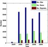 |
Fig. 1 Number of FEROS observations per year for analysis in AMBRE. The 2005 observations begin in October. The number of distinct objects observed and the number with repeated observations are as indicated in the key. |
Figure 1 shows a histogram of the number of FEROS observations per year that were received by OCA, the number for 2005 representing only 3 months of observations. The number counts for the number of distinct objects that have been observed by FEROS in this timeframe and the number with repeated observations are also shown.
The analysis procedure and results for these FEROS spectra are presented in this paper. This analysis has been the testbed for producing many of the tools that will also be used in the analysis of the UVES, HARPS and FLAMES/GIRAFFE archived spectra. These tools have been integrated into an analysis pipeline that feeds the processed spectra into MATISSE for derivation of the spectral parameters.
3. MATISSE and the synthetic spectra grid
MATISSE (MATrix Inversion for Spectral SynthEsis) is an automated stellar parameterisation algorithm based on a local multi-linear regression method. It derives stellar parameters (θ = Teff, log g, [M/H], individual chemical abundances) by the projection of an input observed spectrum on a vector function Bθ(λ), 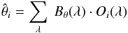 (1)with
  being the derived value. The Bθ(λ) vector function is an optimal linear combination of theoretical spectra, Si(λ), calculated from a synthetic spectra grid.
 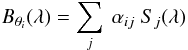 (2)Key features in the observed spectrum due to a particular θ are reflected in the corresponding Bθ(λ) vector indicating the particular regions which are sensitive to θ (Recio-Blanco et al. 2006; Bijaoui et al. 2008).
MATISSE also generates synthetic spectra interpolated to each set of output stellar parameters. For each set of parameters, the synthetic spectrum on the grid, S0(λ), with the closest stellar parameters is identified along with the associated Bθ(λ) function. The Bθ(λ) functions located locally about this point are used to estimate the variations in the flux between the synthetic spectra at the corresponding grid points and the final interpolated synthetic spectrum corresponding to the required stellar parameters (θk) (Kordopatis et al. 2011).
This interpolated spectrum is then used to calculate a χ2 between the interpolated and input normalised spectrum. This provides a measure of the goodness of the fit of the derived stellar parameters to the observed spectrum. Stellar parameters, with log χ2, and corresponding interpolated synthetic spectra are generated for every spectrum that is analysed in MATISSE.
3.1. Grid of synthetic spectra for the classification algorithm
Within the AMBRE Project, the adopted procedure for the automatic classification of stellar spectra relies on a library of reference spectra in order to derive their atmospheric parameters and their chemical abundances. Due to the lack of a library of observed spectra that covers a large range of atmospheric parameters and chemical abundances over a very large spectral domain and resolution, the only solution was to compute large grids of synthetic spectra.
For the AMBRE application, the computed grid of theoretical stellar spectra has to cover the whole optical spectral range at very high resolution in order to be used for the analysis of the majority of the spectroscopic data. For that reason, we have computed a synthetic spectra grid covering the wavelength range between 300 and 1200 nm with a wavelength step of 0.001 nm (900 000 pixels in total) (de Laverny et al. 2012). Since this project is mostly devoted to the analysis of FGKM stars, this grid is based on the latest generation of MARCS model atmospheres presented in Gustafsson et al. (2008). An extension to hotter effective temperatures with Kurucz stellar atmosphere models (Kurucz 1979) is planned for the near future. The considered parameters of the spectral grid are the effective temperature (Teff in K), the stellar surface gravity (log g in dex), the mean metallicity ([M/H] in dex) and the enrichment in α-elements with respect to iron ([α/Fe] in dex).
The metallicity definition here is different to the classical use of [Fe/H] to denote the metallicity of a star. For [Fe/H] the metallicity is defined using the derived abundances from Fe lines only. MATISSE provides the opportunity to use all the available metal lines (those atoms heavier than He) to define a metallicity providing a global metallicity designated as [M/H]. The opportunity also exists with MATISSE to derive a global α element abundance using as many α element spectral lines as possible, where we assumed that in the generation of the synthetic spectra the abundances of the different α elements vary in lockstep. Throughout the AMBRE Project, the following chemical species are assumed to be α-elements: O, Ne, Mg, Si, S, Ar, Ca and Ti, although for any selected wavelength region spectral features for all of these elements may not necessarily be present.
From the selected MARCS model atmospheres, the synthetic spectra were computed with the turbospectrum code (Alvarez & Plez 1998, and further improvements by Plez) in plane-parallel and spherical geometry assuming hydrostatic and local thermodynamic equilibrium. Atomic lines have been recovered from the Vienna Atomic Line Database (in August 2009; Kupka et al. 1999). The molecular line list has been provided by B. Plez. It includes transitions from ZrO, TiO, VO, OH, CN, C2, CH, SiH, CaH, MgH and FeH with their corresponding isotopic variations (see Gustafsson et al. 2008, for a list of references).
This grid covers the following ranges of atmospheric parameters: Teff between 2500 K and 8000 K, log g from −0.5 to + 5.5 dex, and [Fe/H] from −5.0 to + 1.0 dex, although not all combinations of the parameters are available within the grid. The selected MARCS models have [α/Fe] = 0.0 for [M/H] ≥ 0.0, [α/Fe] = +0.4 for [M/H] ≤ −1.0 and, in between, [α/Fe] = −0.25 × [M/H]. For the spectra computation from each of these MARCS models, we considered an [α/Fe] enrichment from −0.4 to + 0.4 dex with respect to the canonical values that correspond to the original abundances of the MARCS models. The final AMBRE synthetic spectra grid consists of 16 783 flux normalized spectra (see de Laverny et al. 2012, for a complete description of this grid).
The microturbulence (ξ) is not a free parameter in this synthetic spectra grid. For the atmospheric models with high log g (+3.5 ≤ log g ≤ + 5.5) ξ is set at 1.0 km s-1. For low log g (log g < + 3.0) ξ is set at 2.0 km s-1, being typical values for dwarfs and giants respectively. These values reflect the MARCS model atmospheres configurations, and further details on the model selection is given in de Laverny et al. (2012). Due to the microturbulence being hardwired into the synthetic grid it was not possible to carry out tests on the effects of variations in ξ on the stellar parameter determination across the whole synthetic spectra grid. However the effects of changes in ξ are most prominent for strong lines. By using the global metallicity [M/H] rather than [Fe/H] we expect the contribution from strong lines on the [M/H] to be negligible due to the significantly larger quantity of non-ξ sensitive small metallic lines.
Section 6 describes the extensive testing of the pipeline that was carried out using observed spectra from which an external error on the resulting parameters is derived by comparison to literature values. To gauge the effect of microturbulence on the derived stellar parameters a key sample of 66 Main Sequence (MS) stars (Bensby et al. 2003), and two key samples of 16 Red Giant Branch (RGB) stars (McWilliam 1990; Hekker & Meléndez 2007) were considered from within the test sample.
The most noticeable effect within the MS sample was an underestimation of the Teff for the hotter MS stars, for which the constant ξ of 1.0 km s-1 underestimates the accepted value. Hence at Teff ~ 6500 K, where Δξ ~ +0.8 km s-1 the effect was ΔTeff ~ −100 K. This is well within the derived Teff external error of 120 K (see Sect. 6).
The most noticeably effect in the RGB sample was on the derivation of log g. At the base of the RGB, where the constant ξ of 2.0 km s-1 is an overestimation, the derived log g was observed to be overestimated by ~0.3 dex for Δξ ~ +0.7 km s-1. At the RGB tip, where ξ = 2.0 km s-1 is an underestimation, log g was observed to be underestimated by ~0.3 dex for Δξ ~ −0.7 km s-1. These variations are within the derived log g external error of 0.37 dex. Hence based on these samples, variations of ξ from the assumed constant values do have an effect on the derived parameters that varies in magnitude with stellar evolutionary stage. However the external error derived from the entire reference sample takes account of them in a global sense (see Sect. 6).
3.2. AMBRE:FEROS subgrid
The FEROS spectra cover most of the optical wavelengths but only a subset of these wavelengths was required for the MATISSE analysis. In order to carry out the MATISSE training phase, where the Bθ(λ) vectors are generated, for the FEROS analysis the optimum resolution, wavelength regions, and sampling of the FEROS spectra were determined. The full AMBRE synthetic spectra grid was then adapted to the same specifications creating the AMBRE:FEROS subgrid that was used in the training phase to generate the AMBRE:FEROS Bθ(λ) vectors.
In this analysis, only Bθ(λ) functions computed from the direct numerical inversion of the correlation matrix (see Recio-Blanco et al. 2006) were considered. These functions are thus not optimized for very low SNR spectra. However, due to the large number of spectral features available in the selected spectral domains, it was not necessary to use the approximated Bθ(λ) functions that are computed with the Landweber algorithm as in Kordopatis et al. (2011). As will be shown in Sect. 5 the estimated internal errors based on the AMBRE:FEROS grid are indeed already very small (see Fig. 10).
3.2.1. Selection of wavelength regions
A detailed analysis of the full wavelength range of the FEROS spectra was undertaken in order to select wavelength regions that would provide the greatest amount of information for each of the derived parameters while also minimising the number of pixels in order to reduce computing time.
FEROS disperses the spectra into 39 orders of varying wavelength interval from ~3500 Å to ~9200 Å at high resolution (R ~ 48 000). The optimum spectral regions for the determination of the stellar parameters were selected taking into account the need to avoid excessive computing time and to avoid low spectral information region. To this end, the signal-to-noise (SNR) per pixel (0.03 or 0.06 Å per pixel for FEROS) as a function of the wavelength was derived for each archived spectra by determining the SNR profile of each spectral order and thus providing a SNR profile over the entire spectral domain. Wavelengths regions with low SNR were rejected, typically the start and end of each order. The wavelengths regions affected by sky absorption and telluric features were also rejected, and also regions where continuum placement proved too difficult owing to wide spectral features in the region. Some key spectral features, such as Hα and the Ca II H & K lines, were also discarded as these features were found to be poorly synthesised based on our current understanding of stellar atmospheres as well as being difficult to normalise automatically.
The remaining spectral regions were then investigated for their intrinsic sensitivity to three of the four stellar parameters to be determined by MATISSE: Teff; log g; and [M/H]. This was carried out using preliminary Bθ(λ) vectors that covered the full optical domain at very high resolution generated using a reduced synthetic grid. Due to the underlying equation for calculating the Bθ(λ) vectors, the high resolution Bθ(λ) vectors could not be simply degraded to lower resolutions to investigate the sensitivity, as this would not accurately reflect the information at that resolution. However the high resolution Bθ(λ) vectors are useful to give a general sense of the sensitivity.
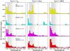 |
Fig. 2 Bθ(λ) sensitivity: number of extrema above 2σ in ~ 200 Å bins against wavelength for four sets of stellar parameters: the Sun; Teff = 6000 K, log g = 2, [M/H] = 0.0; Arcturus; and Teff = 4500 K, log g = 4, [M/H] = −0.5. The Bθ(λ) vectors from left to right are: θ = Teff, log g and [M/H]. The grey stripes represent the final wavelength regions selected for the AMBRE:FEROS analysis (see Table 2). |
For stellar parameters at:
-
1.
Teff = 6000 K, log g = 4.0 dex, [M/H] = 0.0 dex (Sun);
-
2.
Teff = 6000 K, log g = 2.0 dex, [M/H] = 0.0 dex;
-
3.
Teff = 4500 K, log g = 2.0 dex, [M/H] = −0.5 dex (Arcturus);
-
4.
Teff = 4500 K, log g = 4.0 dex, [M/H] = −0.5 dex,
the Bθ(λ) vectors at the same Teff, log g, and [M/H] have been analysed for their extrema distribution. This selection explores the sensitivity of both dwarfs and giants that are similar to the two standard stars, the Sun and Arcturus. The panels in Fig. 2 show how the spectral domain changes in sensitivity with the different stellar parameters. The standard deviation (σ) for each Bθ(λ) vector was calculated as the spread of the pixel values in the Bθ(λ) vector. Then for each Bθ(λ) vector the pixels outside 2σ were binned in ~200 Å bins over the wavelength range from ~4000 Å to ~9500 Å. Hence the bars in Fig. 2 show the number of pixels per bin which have a high sensitivity to the respective θ. Clearly the bluer wavelengths show the greatest sensitivity to all three parameters, reflecting the greater quantity of spectral features in the blue.
This sensitivity to θ for different ranges in θ was used to select the wavelengths regions in the FEROS spectra to be used in the AMBRE analysis. As the greatest sensitivity was located towards the blue, regions were selected, where possible, to capture this sensitivity. The grey regions in Fig. 2 represent the final wavelength regions selected for AMBRE:FEROS which are listed in Table 2. The wavelengths include key spectral features such as the magnesium triplet at ~5160 Å, Hβ (4861 Å), Hγ (4340 Å), Hδ (4101 Å), a CH bandhead (4305 Å) and a CN bandhead (4142 Å) as well as the spectral features for many atomic elements. This wealth of information provided sufficient sensitivity over the range of required stellar parameters in anticipation of the range of spectral types that were potentially included within the FEROS archived sample.
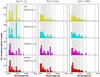 |
Fig. 3 As for Fig. 2 but for the corresponding Bθ(λ) vectors of the AMBRE:FEROS synthetic spectra grid. The y-axis is scaled down compared to Fig. 2. |
FEROS échelle order, starting wavelength and finishing wavelength for each region used in the analysis of the FEROS spectra.
For confirmation of the Bθ(λ) sensitivity, Fig. 3 was generated by the same process as Fig. 2 but using the corresponding Bθ(λ) vectors for the final AMBRE:FEROS grid. Therefore Fig. 3 reflects the sensitivity of the Bθ(λ) vectors at the actual resolution of the AMBRE:FEROS analysis. Due to the reduced number of points in sampling and resolution the 2σ limit is significantly reduced. While some regions show there are subtle differences in the sensitivity of some regions, overall the distribution of greater sensitivity in the blue is in good agreement with the sensitivity at high resolution.
3.2.2. Convolution and sampling of synthetic spectra grid
At the high resolution of R ~ 48 000, the FEROS spectra have typical wavelength sampling (Δλ) of 0.03 Å (1 × 1 binning) or 0.06 Å (1 × 2 binning). The final selected wavelengths corresponded to a total of ~1500 Å and at this sampling this translated to a (maximum) total of ~50 000 pixels. Creating the FEROS synthetic spectra subgrid of ~16 000 spectra at this resolution and sampling would result in excessively large memory and computing requirements when creating the Bθ(λ) vectors in the training phase, and also when loading these vectors during the MATISSSE analysis. It was necessary to reduce the resolution and sampling to a more reasonable pixel total, but without sacrificing the key spectral information. The most reasonable number of pixels per spectra was determined to be ~15 000 in order to ease the use of the available computing power.
By optimising the memory and spectral information requirements, the final specifications for the FEROS synthetic spectra subgrid was determined to be 11 890 pixels with R ~ 15 000 at λ ~ 4500 Å with a sampling of 0.1 Å over ~1500 Å. Hence the full AMBRE synthetic spectra grid (de Laverny et al. 2012) was then sliced to the wavelengths specified in Table 2, convolved by a Gaussian kernel with constant σ and resampled to the optimised FEROS pixels. The training phase was then carried out whereby the Bθ(λ) vectors were generated for use in the MATISSE analysis of the FEROS archived spectra.
4. FEROS analysis pipeline
A complex analysis pipeline (written in shell, Java and IDL) has been built to wavelength slice, radial velocity correct, normalise and convolve the FEROS spectra and then feed them into MATISSE for the determination of their stellar parameters. Figure 4 shows a flowchart of the key stages in the analysis pipeline. The pipeline has been developed so that it can be easily adapted to the remaining three instrument datasets of ESO archived spectra. The following sections outline the procedures carried out for each of the key stages in the pipeline.
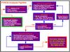 |
Fig. 4 The FEROS Analysis Pipeline: the key stages are displayed in order of analysis. Spectral Processing A and Spectral Processing B carry out testing of spectra quality and preliminary parameter determination, including calculation of the radial velocity and spectral FWHM. In Spectral Processing C robust iterative procedures are carried out resulting in the final stellar parameters and normalised spectra. See text for detailed explanation of each stage. |
4.1. Spectral Processing A: spectra processing for radial velocity determination
Spectral Processing A (SPA) is the initial stage that prepares the FEROS spectra in order to determine the radial velocities. The procedures used here are also used in the later stages of the pipeline. Key flags were defined within the pipeline to be attached to any spectra that satisfied the conditions of the flag. The flags were for “Faulty Spectra” (e.g. missing spectral orders), “Extreme Emission Features” (spectral emission features in the blue with width greater than 50 Å), “Excessive Noise” (extremely noisy spectra with the number of negative flux pixels > 25%) and “Poor Normalisation” (spectra with a total flux above 1.2 > 10%). A spectrum may satisfy multiple flags, particularly in the case of excessive noise which naturally led to poor normalisation. Such types of spectra were unlikely to produce valid results in the MATISSE analysis and as such were rejected from the full analysis. Flags were also implemented to identify “Large Emission Features” (width greater than 1.2 Å) and the presence of odd features that were potentially “Instrumental Relics”. However these flags alone were not enough to reject a spectrum from the full analysis. All of the quality flags were accounted for in the generation of the final dataset of results for ESO, which is explained in Sect. 8.
The first reduction process extracts the required wavelengths (Table 2) from the spectra and then normalises them. However no convolution is carried out so the original resolution is maintained. A hot star spectrum (almost featureless) in the FEROS sample was identified and used to determine a continuum profile for each wavelength region. This profile is divided out of the spectra removing the residual instrument profile and performing a first rough normalisation to place the continuum near unity. At this stage the spectra must necessarily be considered as unknown in stellar parameters and hence the normalisation process must be carried out assuming that key pre-selected continuum regions need to be normalised to unity in intensity. This assumption may not in fact correctly normalise each spectrum. However in these initial stages it is the best, albeit crude, estimate available.
Up to three continuum regions for each wavelength region were pre-selected by an investigation of synthetic spectra and a sample of FEROS spectra covering a range of stellar parameters. For the normalisation, a simple linear profile is constructed for each wavelength region by determination of the mean signal in the respective continuum regions. This profile is divided out of the wavelength region and then the region undergoes cleaning for cosmic rays. The region is scanned for emission features greater than a factor of 1.5 above the noise on the continuum (unity). These features are tested for width and those less than 1.2 Å (40 pixels) are cleaned to unity. Features larger than 1.2 Å (40 pixels) in width are flagged as large emission features and are not cleaned. This limit of 1.2 Å (40 pixels) was determined by an examination of many examples of cosmic rays in the FEROS spectra to get a sense of the number of pixels over which they could be dispersed.
Each wavelength region is treated individually for each spectrum, and the regions are then combined into one vector. This merged spectrum is tested for the goodness of the normalisation and flagged if the normalisation is poor. The resulting spectrum is used in the determination of the radial velocity. At this stage the original resolution is retained. None of the FEROS spectra were rejected at this stage in case later testing and processing recovered a previously rejected spectra (i.e. mis-calculated radial velocity is corrected).
4.2. Radial velocity determination
A completely automatic radial velocity (Vrad) programme has been established that can analyse spectra across a very wide range of stellar parameters and is based on a cross-correlation algorithm that compares the normalised observed spectrum to binary masks (C. Melo, priv. comm.; Melo et al. 2001). To complement this programme a procedure was developed at OCA that computes a set of binary masks to match the observations in terms of wavelength range and resolution, and are used as input to the radial velocity programme. Masks covering the parameter space of the AMBRE:FEROS analysis were computed using synthetic spectra taken from the high resolution, full optical domain, AMBRE synthetic spectra grid (see Sect. 3.1). Six masks for stars hotter that 8000 K were also computed using synthetic spectra from the POLLUX database (Palacios et al. 2010). For the AMBRE:FEROS analysis 51 masks were computed at the stellar parameters given in Table 3. Also listed are 5 standard masks for dwarf stars that were supplied with the radial velocity programme (C. Melo, priv. comm.) and used in the AMBRE:FEROS analysis.
List of the stellar parameters for the binary masks used in the AMBRE:FEROS radial velocity determination that were built from the full AMBRE synthetic grid (45 masks) and the POLLUX database (6 masks).
For each spectrum a cross-correlation function (CCF) ranging from − 500 to + 500 km s-1 was calculated for each of the 56 masks. The CCF was calculated in radial velocity steps (ΔVrad) based on the specified wavelength step (Δλ) of the spectrum. For spectra with Δλ = 0.03 Å the CCF step was calculated to be ΔVrad ~ 1.8 km s-1, and for Δλ = 0.06 Å the CCF step was ΔVrad ~ 3.6 km s-1. For each CCF two separate gaussian fits were made in order to determine the minimum of the profile, and hence the radial velocity. The first fit used the majority of the profile, while the second fit used a section of the profile centred near the mininum with a width equal to the full-width-at-half-maximum (FWHM) of the profile.
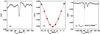 |
Fig. 5 CCFs produced for calculating radial velocities. a) Noisy CCF with an asymmetric profile. b) Core of profile showing skewed full profile gaussian fit (black). The secondary gaussian fit (red) provides a better estimate. c) CCF of the spectroscopic binary, HD 135728, showing two profiles. |
Figure 5a shows an example of a noisy CCF although the key profile is distinct. However, as seen in Fig. 5b, the fit to the full profile (black) provides a minimum skewed away from the actual minimum due to asymmetries of the full profile. The use of the central core of the profile provides a more accurate fit (red). Figure 5c shows an example of a CCF for which two profiles are observed. This is the spectroscopic binary HD 135728. The pipeline selects the most prominent of the two profiles in the determination of the radial velocity. The CCF seems the most likely tool with which to be able to identify the spectra of spectroscopic binaries. However at this stage we have not developed such a routine and so binaries are not specifically detected in the pipeline. The stellar parameters for such spectra are likely to be poorly determined and so will be at least identified as having large associated errors from the radial velocity and stellar parameter analysis. Quality control flags, such as the χ2, may also be used to help identify spectroscopic binaries.
Figure 6 shows the CCF corresponding to the best fit mask for three FEROS spectra at different stellar parameters. The full CCF for each spectrum is shown in the first row, while the second row shows more clearly the profile used to calculate the radial velocity. The full CCF can show varying degrees of noise and gradient depending on the quality of the spectra as is shown in each of these three examples. The respective profiles used to determine the radial velocity reflect the characteristics of the different spectra. The two cooler stars have very prominent inverted peaks, reflecting the numerous spectral lines available with which to make the cross-correlation. The hotter star, with fewer spectral lines, has a much less pronounced profile. These differences can be quantified by the measurement of the contrast of the profile.
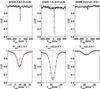 |
Fig. 6 Examples of cross-correlation functions of the best fit masks for three of the FEROS spectra. The first row shows the full CCFs while the second row shows the profiles from which the radial velocities were determined. The final AMBRE:FEROS stellar parameters (Teff,log g, [M/H], [α/Fe]) and radial velocities are stated for each spectrum. The red lines are used to calculate the contrast and FWHM for each profile. |
The contrast was defined here as the amplitude of the profile multiplied by 100 (hence a percentage) where the amplitude of the profile is the length of the vertical red line as shown in each example profile in Fig. 6. The amplitude of the CCF, the continuum placement of the CCF and their associated errors are calculated automatically when using the GAUSSFIT routine in IDL. The sign of the amplitude does change depending on whether the CCF has an absorption or an emission profile. The expected profile in this analysis is an absorption profile.
The two conditions that were required for a profile to have been well fitted by a gausssian were first: the contrast must be less than zero ensuring an absorption profile; and second, the error on the amplitude must be less than 20% of the amplitude ensuring that the CCF profile dominates above the noise. CCFs that satisfied these conditions were considered to be well-defined. Finally the error on the radial velocity (σVrad) was calculated using the prescription outlined in Tonry & Davis (1979). This prescription makes use of the relative heights of the primary and secondary peaks in the CCF profile hence σVrad reflects the goodness of the definition of the primary peak.
The radial velocity programme carried out the calculations for each of the 56 masks, resulting in 56 determinations of the radial velocity for each spectrum. The errors derived from the quality of the gaussian fit and σVrad were used to select the best fit radial velocity. Typically the majority of these determinations were in good agreement at the correct radial velocity. However for masks with parameters far from the true parameters of the star, a radial velocity would be determined that was incorrect but sometimes had sufficiently small errors such that it would be incorrectly selected as the best fit, if the smallest error was the only selection criteria. To avoid this a binning procedure was implemented as follows that discarded such outliers.
For a single spectrum, all of the Vrad determinations with well-defined CCFs were binned by Vrad into a maximum of 3 bins in correlation with the overall spread of the Vrad values. The bin size was set in each instance by the difference in the maximum and minimum Vrad values divided by the number of bins. The bin with the largest number of members was retained and the outlying bins were discarded. The Vrad within accepted bin with the smallest σVrad was selected as the final Vrad. In the case of an equal number of members within 2 or more bins, the bin with the smallest spread in Vrad values (so best agreement) was selected. Typically, most of the radial velocities for a spectrum were in good agreement, so the maximum bin was easily identified. Otherwise the radial velocities were highly dispersed, and this would be reflected in the σVrad of the final selected value.
The errors on the gaussian fit of the CCF and the σVrad values were used later in the analysis pipeline to identify problematic spectra and select alternate radial velocities where necessary, and also as quality criteria for the final set of results to be delivered to ESO.
The S4N (Allende Prieto et al. 2004) and Crifo et al. (2010) libraries provided good samples of stars with which to validate the radial velocities determined in the AMBRE:FEROS pipeline. The S4N library comprises of 118 F and G dwarf stars for which a detailed analysis was carried out using high resolution high SNR spectra. All four parameters (Teff,log g, [Fe/H] and [α/Fe]) as well as radial velocities are available for each of the S4N stars. Crifo et al. (2010) is the preliminary list of 1420 candidate standard stars to be used to calibrate the radial velocities obtained with Gaia RVS. Section 6 gives further discussion on the use of these libraries to validate the AMBRE:FEROS results.
Within the FEROS archived dataset 30 stars (338 spectra) were found that are also within the S4N library, and 183 stars (411 spectra) were found that are also within Crifo et al. (2010). Figures 7a and b compare the S4N and Crifo et al. (2010) radial velocities values with those determined for AMBRE:FEROS. The mean and standard deviation of the differences between the two sets for each sample are also shown. There is a small offset in both sets with the S4N having a greater offset of 1.8 ± 1.4 km s-1 compared to Crifo et al. (2010) of 0.52 ± 0.35 km s-1. The FEROS spectra were sampled at either 0.03 Å or 0.06 Å from the ESO:FEROS reduction pipeline corresponding to expected Vrad accuracies of 1.6 km s-1 and 3.3 km s-1 respectively. Hence these offsets indicate very good agreement for both samples, particularly for the Crifo et al. (2010) values.
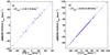 |
Fig. 7 Comparison of AMBRE:FEROS radial velocities: a) S4N library for 29 stars (338 spectra); and b) Crifo et al. (2010) for 158 stars (318 spectra). |
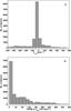 |
Fig. 8 Histogram of the radial velocity values calculated for all of the FEROS archived spectra defined as good spectra with well-defined CCFs: a) Vrad; and b) FWHM of the Vrad CCF. |
All of the FEROS spectra were analysed for their radial velocity. However for 4217 spectra (19.6%) poorly defined or non-standard CCFs lead to unreliable estimates of the radial velocity. This is most likely due to some peculiar or non-stellar properties of the spectra (i.e. nova). Of these 4217 spectra, 549 also failed the conditions of the rejection flags as defined in Sect. 4.1.
Figure 8a is a histogram of the radial velocities calculated for the FEROS spectra defined as good quality with well-defined CCF (15 513 spectra). The majority of the spectra have radial velocities between − 100 and + 50 km s-1. Figure 8b is a histogram of the FWHM of the CCF, calculated from the full CCF profile, for the same sample of spectra. It shows that the majority of spectra returned a FWHM of less than 50 km s-1. The effects of the CCF on the selection of the final dataset will be discussed in Sect. 8.
4.3. Spectral Processing B: spectra reduction, convolution and first parameter estimation
Spectral Processing B (SPB) proceeds under two iterations through the normalisation procedure and the MATISSE analysis. These are necessary as key tests on the normalisation and radial velocity correction are carried out between the two iterations allowing alterations to be made that provide better first estimates of the stellar parameters for the remaining pipeline procedures. For both iterations the original archived spectra are re-analysed using the same procedures as outlined in SPA in terms of wavelength selection, cosmic ray cleaning and normalisation. However in both iterations of SPB the measured Vrad correction is automatically applied to each spectrum prior to normalisation. This allows each spectrum to be shifted to the laboratory rest frame at which the synthetic grid, and so the Bθ(λ) vector functions, have been calculated.
The AMBRE:FEROS synthetic grid was set to a resolution lower than the resolution of the observed FEROS spectra. In order to convolve the observed spectra to the appropriate resolution three factors needed to be taken into account. First, the observed spectra are observed with constant resolving power, which corresponds to increasing FWHM of the spectral features with wavelength. Second, the synthetic spectra grid was convolved using a gaussian profile with constant FWHM hence the synthetic spectra have constant spectral FWHM with wavelength, not a constant resolution. Third, the construction of the full AMBRE synthetic spectra grid did not include astrophysical broadening such as those due to Vsini and ξ (de Laverny et al. 2012). Hence a straight-forward convolution using the nominal instrument FWHM and the FWHM applied to obtain the AMBRE:FEROS synthetic spectra grid would result in convolved observed spectra that had increasing FWHM with wavelength in disagreement with the synthetic spectra. Also for stars with astrophysical broadening greater than the broadening due to the resolving power of the instrument the spectra would be too broad for the appropriate parameter range of synthetic spectra.
Therefore a procedure was implemented that measured the spectral FWHM for each of the 17 selected wavelength regions (see Table 2) for each spectrum and then applied an appropriate gaussian profile to smooth each wavelength region in order that the convolution resulted in observed spectra that had spectral FWHM as close as possible to the constant FWHM of the synthetic spectra grid.
The FWHM values were measured as part of SPB and this was found to significantly increase the processing time of this stage of the pipeline. Hence, due to it being primarily a testing phase, for the first iteration of SPB the observed spectra are convolved using predetermined “mean” spectral FWHM values that were determined for each of the 17 wavelength regions. These default spectral FWHM values were determined by a statistical analysis of a subsample of 384 of the FEROS archived spectra, whereby the FWHM for as many weak and medium strength spectral lines as possible were measured in each of the sample spectra.
The FWHM was measured by fitting a gaussian function to each spectral feature and calculating the width of the gaussian profile at the midpoint of the depth of the profile. For each spectrum the FWHM values increased with wavelength hence assuming one FWHM for the entire spectrum was not reasonable across the wavelength domain of the AMBRE:FEROS analysis. Hence a mean FWHM value for each of the 17 wavelength sections was determined and these were used in the convolution of the corresponding wavelength section. The convolution was carried out using a transformation gaussian profile for which the standard deviation (σX) was defined as: 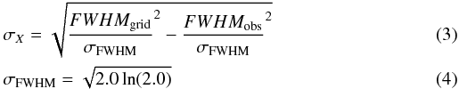 \arraycolsep1.75ptwhere FWHMobs is the default FWHM for the region, FWHMgrid = 0.33 mÅ and σFWHM transforms the FWHMs to σs. Therefore each region of the observed spectrum was convolved such that the FWHM of the convolved spectrum matched the FWHM of the synthetic spectrum.
Part of the convolution process is to resample the observed spectra to the same wavelength bins as the FEROS synthetic spectra grid. Also for SPB, the same quality tests outlined in SPA are used but again no spectra were rejected based on these tests in this first iteration.
The convolved FEROS spectra were then analysed using MATISSE to obtain the first estimate of the stellar atmospheric parameters (Teff, log g, [M/H] and [α/Fe]). MATISSE also outputs synthetic spectra interpolated to the derived stellar parameters. Within the MATISSE algorithm the determination of the stellar parameters undergoes 10 iterations during which the algorithm converges on the final parameters for each spectrum. This number is set empirically and the majority of spectra converge to their parameters in much less than 10 iterations. After the MATISSE analysis is complete each spectrum is tested for whether convergence on the final Bθ(λ) function occurred within the 10 iterations and also the spectrum is tested as to the goodness of the fit between the normalised and the interpolated synthetic spectra in a log (χ2) calculation. In the case of non-convergence within MATISSE, the parameters determined at the ninth and tenth iterations are compared and the solution with the lowest log (χ2) is selected as the final set of parameters. If there is no convergence and/or a high log (χ2), the spectra are flagged for further investigation. The majority of these instances were attributable to incorrect selection of the radial velocity. A separate routine was developed that carries out an automated visual inspection of these spectra in order to select, where possible, an improved radial velocity correction from the full list of radial velocity masks. In some instances the normalisation of the spectra was poor due to noisy spectra, strange spectral features or an invalid radial velocity correction. In the latter case the adjustment to the radial velocity would correct the poor normalisation. In the former cases these spectra were captured by quality/rejection flags in the normalisation process or in the construction of the final ESO dataset.
After these adjustments were made the spectra were reprocessed in the second iteration of SPB. This process is exactly the same as the first iteration except the mean spectral FWHM of the absorption lines for each wavelength section is now measured directly for each individual spectrum. This second iteration of SPB provides the first scientific estimate of the parameters, and hence convolving the spectrum with spectral FWHM values measured specifically for each spectrum provides a more robust analysis. The measured spectral FWHM values were used to convolve each region of each spectrum to match the FWHM of the AMBRE:FEROS synthetic spectra grid. Therefore in Eq. (3) the FWHMobs is the measured spectral FWHM for each wavelength section for each spectrum.
Extensive testing was carried out which compared spectral lines that were in common between the observed and synthetic spectra both before and after convolution in order to ensure that the transformation calculation resulted in appropriately convolved observed spectra. This included testing the procedure on the original high resolution synthetic spectra to ensure the AMBRE:FEROS resolution was obtained after convolution by this procedure. The FWHMgrid (0.33 mÅ) was calculated based on a sample of the AMBRE:FEROS synthetic spectra for which the FWHM values were determined by the same method as for the observed spectrum and were found to be constant with wavelength as expected due to how the synthetic spectra were generated. This ensured consistency in the calculation and application of the FWHM in the convolution process.
Part of the calculation of the spectral FWHM was to classify each spectrum using the number of spectral lines and the widths that were measured. Three categories were used: “Weak” for less than 25 lines measured which were typically found to have FWHM < 0.11 (FWHMweak) and were generally noisy spectra; “Medium” for more than 25 lines measured, where the line depths of the measured lines were between 0.5 and 0.95 in normalised intensity, and no more than 1 strong line was identified (FWHMmedium); and “Strong” for more than 1 strong line identified where the line depth of the “Strong” line was between 0.35 and 0.5 of the normalised intensity (FWHMstrong). The spectral lines were identified by locating the minima and maxima in the spectra, fitting a gaussian at each minima and then discarding those lines which failed the quality tests of the gaussian fit. For a spectrum typically classified as FWHMmedium 1000 to 2000 lines were identified which were reduced to ~400 lines with good gaussian fits.
The “Strong” classification was an attempt to identify the spectra with large, broad spectral features as this provided another estimate of the spectral classification of the star. This was accomplished by applying a high FWHM smoothing function to each spectrum and then testing for which spectral features still remained. A spectrum without “Strong” lines would be reduced to a line near the continuum, while “Strong” features would otherwise still be prominent. This method had to be tailored to the FEROS wavelength region in order to place relevant limits on the possible number of “Strong” lines and their location within the wavelength regions. If, by this method, more than 1 “Strong” line were found then the spectrum was classifed as FWHMstrong and the mean spectral FWHM of the “Strong” lines was recorded.
In the cases where the spectrum was designated as FWHMweak or FWHMstrong, then default spectral FWHM values were used instead. The spectral FWHM values for each spectrum that were used in the convolution, measured or mean values, were saved to an external file to be used in the next stage of the pipeline. Extensive testing was carried out using corresponding spectral lines in the original, convolved and synthetic spectra to confirm that the spectral FWHM procedure correctly convolved the archived spectra to the resolution of the synthetic grid across the wavelength range.
At this stage the spectra which failed the tests identifying un-analysable spectra (extreme emission features, extreme noise-dominated spectra etc.) were rejected from the analysis process. This reduced list was analysed once more in MATISSE in order to determine the first estimate of the stellar parameters to be used in the next stage of the analysis pipeline. The convergence and log χ2 were tested again to catch any further mis-identified radial velocity corrections. At the end of the second iteration of SPB 2370 FEROS spectra were rejected, 11% of the total number of FEROS archived spectra.
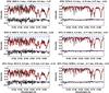 |
Fig. 9 Normalisation procedure for a two stars with Teff ~ 4600 K (left) and Teff ~ 5300 K (right) shown by the wavelength region about two lines of the magnesium triplet. Top: the second iteration of SPB, middle: first iteration of SPC, and bottom: final solution from SPC. The stellar parameters (Teff, log g, [M/H] and [α/Fe]) and goodness of fit over all the AMBRE:FEROS wavelengths (log χ2) are shown. The synthetic spectrum interpolated to these parameters is shown in red, while the normalised observed spectrum is shown in black. The difference between observed and synthetic spectra is also shown at 0.0. |
4.4. Spectral Processing C: iterative spectra normalisation and parameterisation
The final number of FEROS spectra that were passed to the final stage of the analysis pipeline, Spectral Processing C (SPC), was 19 181. SPC again uses the same procedures as SPA and SPB with two differences. The first difference is that the spectra are convolved using the spectral FWHM values determined in the second iteration of SPB rather than re-measuring the FWHM. The second difference is the use of a more robust method for the normalisation of the spectra.
Previously, in SPA and SPB, a “rough” normalisation process was carried out that used pre-selected continuum regions to normalise the spectra to unity. But this is an invalid assumption for many stars, in particular for cool stars which have depressed continuum regions due to molecular bandheads that should not be normalised to unity. However at the beginning of SPC we have an estimate of the stellar parameters from the second iteration of SPB that gives us some valid information about each spectra that we did not previously possess.
We take advantage of this information by using the interpolated synthetic spectra generated for each set of stellar parameters as a better estimate of the continuum placement for the normalisation of the observed spectra. In an iterative process that discards absorption and emission features by polynomial fitting and sigma clipping to leave only “continuum” regions, the synthetic spectrum is divided out of the corresponding observed spectrum leaving a residual of continuum points. A continuum profile is fitted to this residual which is then divided out of the observed spectrum, normalising it to a pseudo-continuum that better represents the parameters of the star. This process overrides any residual curvature that remains after, or was introduced by, the normalisation to the hot star continuum.
These pseudo-continuum normalised spectra are reanalysed in MATISSE to obtain a second estimate of the stellar parameters and another set of synthetic spectra. The “normalisation treatment & MATISSE analysis” cycle is repeated 9 times, which had been determined to be a sufficient number of iterations within which the normalised spectra and stellar parameters could converge to their optimum state. This typically occurred within five iterations. This approach provides a robust incremental adjustment of the parameters and normalisation process that hones in on a realistic estimate of the stellar parameters of each spectra, a process which is not possible using the normalisation method of SPA and SPB.
Figure 9 shows the normalisation procedure for two FEROS spectra in the wavelength region about two of the magnesium triplet at 5160 Å as an example of depressed continuum regions. The two stars correspond to temperatures of Teff ~ 4600 K (SNR = 115) and Teff ~ 5300 K (SNR = 204) respectively. For each spectrum the normalisation by SPB, the first iteration of SPC and the final solution that was found in SPC are shown. The stellar parameters and log χ2 (which is calculated over all the AMBRE:FEROS wavelengths) determined at each stage are shown as well as the synthetic spectrum interpolated to the stellar parameters. The difference between the observed and synthetic spectra is also included to show how it converges.
For the cooler star this rough normalisation of SPB is not a good fit as the observed spectrum is set too high compared to the synthetic spectrum generated at the corresponding stellar parameters. This shows how inadequate normalisation to unity is for cool star spectra. However the rough normalisation does provides a reasonable fit to the synthetic spectrum for the hot star although the placement of the continuum is still not ideal.
At the initial iteration of SPC the spectrum undergoes its first normalisation to the previous solution synthetic spectrum. For the cooler star the observed spectrum now sits below unity in better agreement with the new synthetic spectrum, but there are still mismatches in the relative placement of the two spectra and the line depths. For the hotter star there is very good agreement between the observed and synthetic spectra. In both cases the improvement in the match are shown by the lower log χ2 values.
The final solution for the cooler star (i = 6) shows excellent agreement between the observed and the synthetic spectra, which is reflected in the much lower log χ2 value. Indeed the visual inspection of the spectra show that they are in good agreement in this section of wavelength. For the hotter star the solution (i = 7) is very close to the solution determined in the first iteration of SPC, indeed the log χ2 does not change. Visually this good fit is obvious between the observed and synthetic spectra. The comparison of these two stars illustrates the greater difficulty there is in the normalisation and parameterisation of cool stars. However the procedure developed for the AMBRE pipeline can successfully manage both cases and the normalisation procedure in SPC is particularly effective in the case of cool stars where the continuum regions are more heavily obscured by spectral features.
Typically convergence occured by the fourth or fifth iteration of the normalisation and stellar parameter determination cycle. When convergence has occurred the final set of parameters are selected as those from the converged solutions with the lowest log (χ2). In the case of non-convergence within the 9 iterations of SPC, it is assumed that for the final six iterations any bias introduced by the initial rough normalisation has been erased. Of these final six iterations the solution with the lowest log (χ2) is selected as the final stellar parameters for the spectra along with the corresponding normalised and synthetic spectra.
Hence the radial velocity, stellar parameters (Teff, log g, [M/H] and [α/Fe]), normalised spectra and corresponding inteprolated synthetic spectra were determined in SPC for 19 181 of the 21 551 FEROS spectra.
Extensive testing of the FEROS analysis pipeline was carried out in order to optimise the procedures and to validate the MATISSE results by making comparison to literature values. The following sections describe the different tests and validations that were carried out.
5. AMBRE:FEROS internal error analysis
The internal errors can be used to determine how well MATISSE will derive the stellar parameters of similar stellar types which have different levels of noise and different uncertainties in radial velocity. In order to test for noise and radial velocity effects a sample of 500 synthetic spectra were generated at random stellar parameters covering the entire stellar parameter range, spectral resolution and wavelength domains of the AMBRE:FEROS synthetic spectra grid.
5.1. Internal errors: SNR
To test the effects of noise the sample of synthetic spectra was reproduced five times by adding differing levels of noise per pixel (0.1 Å per pixel for AMBRE:FEROS synthetic grid) at SNR = 10, 20, 50, 100. Each sample was then re-analysed in MATISSE and the derived stellar parameters were compared to the original values.
Figures 10a to d show how the difference in stellar parameters changes with increasing SNR for Teff, log g, [M/H] and [α/Fe] respectively. For each noise-added sample the difference between the original and derived parameters was calculated and then the difference value at the 70th percentile (~1σ) was determined. For example, in Fig. 10a at a SNR of 10 (the noisiest), 70% of the synthetic spectra returned Teff values within 14 K of the original Teff value. At a SNR of 100, 70% of the sample returned values within 2 K of the original Teff value. Similarly small errors were also found for log g, [M/H] and [α/Fe] that diminished to negligible levels at SNR of 100 in all cases. This analysis shows that for two synthetic spectra with very similar intrinsic stellar parameters, where the differences in the spectra are only attributable to noise, MATISSE will determine close to the same stellar parameters indicating that the internal errors of MATISSE are very small. This can be attributed to the large wavelength coverage and high resolution of the FEROS spectra which contain a great deal of information on the stellar parameters in terms of spectral lines, even at low SNR, of which MATISSE takes advantage.
Overall this analysis shows that the internal error due to SNR is negligible in the FEROS results. The internal (int) error on each parameter due to SNR (σint,snr) is calculated as part of the MATISSSE programme. It was used to calculate the total internal error as explained at the end of this section.
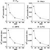 |
Fig. 10 Internal error for each parameter with changes in SNR. a) The ΔTeff that 70% of the synthetic sample were less than or equal to when calculating the difference between the nominal Teff and the Teff determined for the respective SNR. b) As for a) but for log g. c) As for a) but for [M/H]. d) As for a) but for [α/Fe]. |
5.2. Internal errors: Vrad and V sin i
A similar investigation was carried out in order to determine the effect of uncertainties in radial velocity on the determination of the stellar parameters by MATISSE. The sample of interpolated spectra were reproduced this time undergoing radial velocity shifts of ΔVrad = 0, 0.5, 1.0, 5 and 10 km s-1 with an SNR of 100. Figures 11a to d show how the difference in stellar parameters changes with increasing radial velocity uncertainty for Teff, log g, [M/H] and [α/Fe] respectively. Again the difference between the original and derived stellar parameters was obtained and the difference value at the 70th percentile for each sample was calculated. At a radial velocity uncertainty of 5 km s-1 (~0.09 pixels) the error in stellar parameter determination becomes significant ( > 1%) for each of the stellar parameters. However if the uncertainty in the radial velocity is less than 5 km s-1 the MATISSE parameters compare well to the true values.
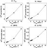 |
Fig. 11 Internal error for each parameter with changes in the Vrad uncertainty (km s-1). a) The ΔTeff that 70% of the synthetic sample were less than or equal to when calculating the difference between the nominal Teff and the Teff determined for the respective Vrad uncertainty. b) As for a) but for log g. c) As for a) but for [M/H]. d) As for a) but for [α/Fe]. |
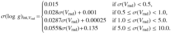
The internal uncertainty in each stellar parameter due to radial velocity was calculated using the equations that connect the points in Fig. 11. The error on the radial velocity, σ(Vrad), determined in the radial velocity programme was used as the input to determine the internal error due to the Vrad uncertainty (σint,Vrad) for each parameter for each spectrum according to the following conditions: 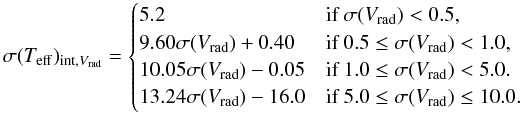
![Mathematical equation: \begin{equation*} \sigma([\text{M/H}])_{{\rm int},{V}_{\rm rad}}\!=\! \begin{cases} 0.008 & \text{if }\sigma({V}_{\rm rad}) < 0.5, \\ 0.012 \sigma({V}_{\rm rad}) + 0.002 &\text{if }0.5 \leq \sigma({V}_{\rm rad}) < 1.0 , \\ 0.0213 \sigma({V}_{\rm rad}) - 0.0073 &\text{if }1.0 \leq \sigma({V}_{\rm rad}) < 5.0. \\ 0.0510 \sigma({V}_{\rm rad}) - 0.156 &\text{if }5.0 \leq \sigma({V}_{\rm rad}) \leq 10.0. \end{cases} \end{equation*}](/articles/aa/full_html/2012/06/aa18829-12/aa18829-12-eq100.png)
![Mathematical equation: \begin{equation*} \sigma([\alpha\text{/Fe}])_{{\rm int},{V}_{\rm rad}}\!=\! \begin{cases} 0.006 & \text{if }\sigma({V}_{\rm rad}) < 0.5, \\ 0.010 \sigma({V}_{\rm rad}) + 0.001 &\text{if }0.5 \leq \sigma({V}_{\rm rad}) < 1.0 , \\ 0.0128 \sigma({V}_{\rm rad}) - 0.0018 &\text{if }1.0 \leq \sigma({V}_{\rm rad}) < 5.0. \\ 0.0204 \sigma({V}_{\rm rad}) - 0.0400 &\text{if }5.0 \leq \sigma({V}_{\rm rad}) \leq 10.0. \end{cases} \end{equation*}](/articles/aa/full_html/2012/06/aa18829-12/aa18829-12-eq101.png) The rotational velocity (Vsini) of a star can have an impact the broadening of the observed spectral features depending on the magnitude of the rotational velocity and the resolution of the instrument. The AMBRE synthetic spectra grid was generated with no variations in Vsini, assuming all stars to be slow rotators. However it is important to consider whether variations in Vsini will have an effect on the determined stellar parameters. Gazzano et al. (2010) carried out a robust investigation into the Vsini limits of reliable stellar parameter determination using MATISSE and found that spectra with Vsini < 11 km s-1 produced good results in the MATISSE analysis of a sample of FGK dwarfs. Based on this, Gazzano et al. (2010) accepted all CCF FWHM ≤ 20 km s-1 for spectra at a resolution of R ~ 26 000. The FEROS sample and the AMBRE synthetic spectra grid are of much broader range in stellar parameters and wavelength, and of lower resolution (R ~ 15 000) than the Gazzano et al. (2010) study. Hence the effects of Vsini on the range of stars for which the synthetic grid has been optimised, would be well-masked for the AMBRE:FEROS configuration. In Sect. 7.2.3 we examine the FEROS sample in the context of the CCF FWHM to identify spectra which are not well-represented by the AMBRE synthetic spectra grid.
The rotational velocity (Vsini) of a star can have an impact the broadening of the observed spectral features depending on the magnitude of the rotational velocity and the resolution of the instrument. The AMBRE synthetic spectra grid was generated with no variations in Vsini, assuming all stars to be slow rotators. However it is important to consider whether variations in Vsini will have an effect on the determined stellar parameters. Gazzano et al. (2010) carried out a robust investigation into the Vsini limits of reliable stellar parameter determination using MATISSE and found that spectra with Vsini < 11 km s-1 produced good results in the MATISSE analysis of a sample of FGK dwarfs. Based on this, Gazzano et al. (2010) accepted all CCF FWHM ≤ 20 km s-1 for spectra at a resolution of R ~ 26 000. The FEROS sample and the AMBRE synthetic spectra grid are of much broader range in stellar parameters and wavelength, and of lower resolution (R ~ 15 000) than the Gazzano et al. (2010) study. Hence the effects of Vsini on the range of stars for which the synthetic grid has been optimised, would be well-masked for the AMBRE:FEROS configuration. In Sect. 7.2.3 we examine the FEROS sample in the context of the CCF FWHM to identify spectra which are not well-represented by the AMBRE synthetic spectra grid.
5.3. Internal errors: normalisation
The effects of normalisation on the MATISSE determination were measured using the iterative normalisation process (SPC) of the FEROS analysis pipeline. Using a test sample of 384 FEROS spectra ( ⟨ SNR ⟩ = 100 ± 45) the changes in normalisation between iterations of SPC was explored.
Figure 12 shows the progression of the goodness of fit between the reconstructed spectra and the normalised spectra at each iteration of SPC as a Box & Whisker graph. Assuming that by the 9th iteration convergence has occured, the absolute difference in the log χ2 between the 9th and ith iteration was calculated for each of the 384 test spectra. The spread in values is largest at i = 0 and there is a large decrease in the spread for i = 1. The following iterations show a more sedate decrease in spread and appear to have converged from i = 6.
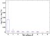 |
Fig. 12 Box & Whisker graph of the absolute difference in the log χ2 of the reconstructed to the normalised spectra for the 384 test spectra between the 9th SPC iteration and each of the previous iterations ( | log χ2(9) − log χ2(i) | ). The box is constrained by the 25th and 75th percentiles, and the red lines are the medians. The whiskers extend to the furthest data points not considered to be outliers. |
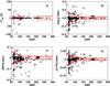 |
Fig. 13 Internal error with changes in Normalisation for a) Teff; b) log g; c) [M/H]; and d) [α/Fe]. The red lines are determined as the 2σ uncertainty on values in two SNR bins (ΔSNR ≈ 30) centred at SNR = 65 and 100 and constant uncertainty for SNR > 125. |
To measure the internal error associated with the normalisation process we investigated the difference in stellar parameters between the 9th and 7th iteration for the test sample. Hence we assumed that the solutions have converged from at least the 7th iteration and the subsequent variations in the stellar parameters are due to minor adjustment of the normalisation of the observed spectra. The variation from convergence (i = 7) to the final iteration (i = 9) was used to give the internal error due to the normalisation process.
Figure 13 shows the difference in each stellar parameter between the 9th and 7th iterations against SNR for the 384 test spectra as black points. These values were binned into two SNR bins (ΔSNR ≈ 30) centred at SNR = 65 and 100, and a single bin for all points with SNR > 125. The 2σ uncertainty for each bin is shown as red squares at the bin centre. Red lines connect the bin uncertainty values. For Teff the spread is constant for each bin and so a constant value for the internal uncertainty due to normalisation was adopted. For log g, [M/H] and [α/Fe] the spread diminishes with increased SNR until SNR = 125 after which a constant spread is found. The adopted internal errors for these three parameters were therefore a piecewise function of SNR. The following equations define the internal errors due to normalisation for each parameter (σint,norm): 
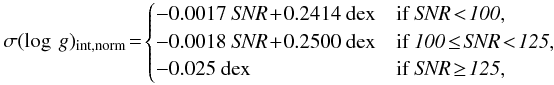
![Mathematical equation: \begin{equation*} \sigma(\text{[M/H]})_{\rm int,norm}\!=\! \begin{cases} -0.0007 {\it ~SNR} \!+\! 0.0964 \text{~dex} & \text{if }\it SNR \!<\! 100,\\ -0.0004 {\it ~SNR} \!+\! 0.0690 \text{~dex} & \text{if }\it 100 \!\leq\! SNR \!<\! 125,\\ -0.014 \text{~dex} & \text{if }\it SNR \!\geq\! 125,\\ \end{cases}\\ \end{equation*}](/articles/aa/full_html/2012/06/aa18829-12/aa18829-12-eq121.png)
![Mathematical equation: \begin{equation*} \sigma([\alpha/\text{Fe]})_{\rm int,norm}\!=\! \begin{cases} -0.0006 {\it ~SNR} \!+\! 0.0671 \text{~dex} & \text{if }\it SNR \!<\! 100,\\ -0.0002 {\it ~SNR} \!+\! 0.0260 \text{~dex} & \text{if }\it 100 \!\leq\! SNR \!<\! 125,\\ -0.006 \text{~dex} & \text{if }\it SNR \!\geq\! 125,\\ \end{cases}\\ \end{equation*}](/articles/aa/full_html/2012/06/aa18829-12/aa18829-12-eq122.png)
5.4. Total internal error
The internal errors due to the SNR, Vrad and Normalisation calculated above were combined in quadrature to give the total internal error for each parameter (σ(θ)int) for each spectrum. This was calculated as follows:  (5)These values were reported for each spectrum in the ESO dataset as described in Sect. 8.
6. AMBRE:FEROS external error analysis
The external error was quantified by comparing the AMBRE:FEROS stellar parameter values to literature values for key reference stars that exist within the AMBRE:FEROS dataset.
List of standard stars and the corresponding spectral atlases used to test the FEROS analysis pipeline.
A list of stars that had been observed with FEROS but were also part of other high quality spectroscopic studies were identified and this reference sample was used to provide quality criteria for each derived stellar parameter. Unfortunately, reference stars covering the whole range of possible parameters could not be found in the literature. In several cases, estimates of the mean stellar metallicity were lacking and the situation was even worse for the [α/Fe] chemical contents since too few reference stars with known [α/Fe] content could be found in the literature.
6.1. Building the FEROS reference sample
In order to compare the MATISSE stellar atmospheric parameters to the literature and to define some quality criteria, a list of reference stars was built using key spectral atlases and libraries.
6.1.1. Stellar atlases: Sun, Arcturus, Procyon
Table 4 lists the standard stars and the corresponding stellar atlases that were used to test the FEROS analysis pipeline. Of these atlases only the S4N solar atlas was observed using FEROS. However the adaptability of the pipeline meant that the use of spectra from other instruments presented no difficulty as long as the required wavelength ranges were available. The accepted stellar parameters for each standard star are listed in bold in Table 4. The final stellar parameters that have been derived in the AMBRE:FEROS analysis with bias corrections (see end of this section) for each atlas are also given.
These atlases were combined in a test sample that included high resolution synthetic spectra for the Sun and Arcturus, as well as synthetic spectra for each grid point in the AMBRE:FEROS synthetic grid corresponding to the Sun and Arcturus. These were used to check the internal consistency of the pipeline in terms of normalisation and convolution of the input spectra. The results for the Sun are in very good agreement with the accepted values. For Arcturus we over-estimate the Teff and log g values however we are within 2σ of the accepted values for Teff. For Procyon there is good agreement in Teff and log g, although the Teff is slightly under-estimated within the stated external errors. However the metallicity is under-estimated by − 0.25 dex which is outside the 2σ limit. The under-estimation of the Teff may account for some of this discrepancy in metallicity. However further investigation into understanding the variation in the stellar parameters for these standard stars is ongoing.
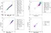 |
Fig. 14 Comparison of stellar parameters determined in AMBRE:FEROS (A:F) and the reference sample (RS) from PASTEL: a) Teff; b) log g; c) [M/H] compared with [Fe/H]; d) [α/Fe]. The legend identifies the relevant individual papers and the associated sample bias ± σ. The stellar atlases are also shown. The dashed line indicates a 1:1 agreement. The axis limits represent the limits on the final accepted parameters. |
6.1.2. Spectral libraries reference sample
Preliminary investigations showed that merely making comparison between the MATISSE results and all of the stellar parameter values that were available in SIMBAD for the FEROS stars resulted in a great deal of disparity. There was no quality determination on the values with which we made the comparison. Homogeneously analysed large sample datasets were necessary in order to ensure that a valid comparison was being made. To this end key spectral libraries were investigated in order to locate within the FEROS archive dataset stars that had been analysed in high quality studies. This list of spectral libraries is given in Table 5.
List of spectral libraries used to select comparison stars from the FEROS archived spectra.
The primary spectral library that was used was the PASTEL database (Soubiran et al. 2010)3, which provides a selection of key papers that carried out detailed spectroscopic studies at high resolution and high SNR to derive high quality stellar parameters. From these papers we were able to identify a total of 148 stars corresponding to 618 FEROS archived spectra (Table 5). There was significant crossover of stars between the studies which provided another level of comparison for this work. From the PASTEL sample ~120 stars (~300 spectra) had values for three stellar parameters, Teff,log g and [Fe/H], while the remaining stars had Teff values only. In the following comparison we assume the literature values to be correct. However we note that the literature values, while they are high quality studies, were determined using a range of techniques (Soubiran et al. 2010), in particular, several studies determined photometric Teff values using the Infra-Red Flux Method (Alonso et al. 1996, 1999; Ramírez & Meléndez 2005; González Hernández & Bonifacio 2009).
Figures 14a to b compare the Teff, log g, [M/H] and [α/Fe] values determined by AMBRE:FEROS with the literature values of the reference sample and stellar atlases. The legend in each provides the bias and σ for each subsample. The axes represent the limits of the final accepted parameters and clearly the reference sample does not cover the entire grid as would be ideal. Despite this limitation the reference sample was sufficient to define bias corrections which were necessary to apply to the AMBRE:FEROS stellar parameters.
6.1.3. Reference sample: Teff
Figure 14a compares the Teff for each star. It is important to note that many of the literature Teff values were not determined spectroscopically, as stated above. Despite the differences in measurement technique, overall there is excellent agreement between the AMBRE:FEROS results and the PASTEL values, and also good agreement for the stellar atlases. There is a slight turning over of the distribution from Teff ≳ ~ 5750 K for which a small bias correction was applied that will be quantified at the end of this section.
6.1.4. Reference sample: log g
Figure 14b shows the comparision of the log g values for which there is reasonably good agreement. However the majority of the sample are dwarfs (high log g), and the giants (low log g) are under-represented. There is a slight gradient within the sample which resulted in a small bias correction being applied at high log g for the final results (see end of the section). The lack of a significant sample of giants made it difficult to accurately define a bias at low log g, hence the correction was only applied at high log g. However the uncertainty on the giants is definitely higher.
6.1.5. Reference sample: [M/H]
Figure 14c shows the comparison of the AMBRE:FEROS [M/H] values with the literature [Fe/H] values. The difference in definition between [M/H] and [Fe/H], as discussed previously, means that this is not an accurate comparison, as so many more elements (albeit of lesser contribution) than just Fe are included in the MATISSE metallicity. The comparison shows an overall systematic offset between the AMBRE:FEROS and literature values reflected in the subsample biases. The sources of this bias are difficult to quantify so we assumed a direct comparison between [Fe/H] and [M/H] then made a systematic bias correction to the final [M/H] results as outlined at the end of this section.
6.1.6. Reference sample: [α/Fe]
Unfortunately very few comparison stars with published values of their [α/Fe] exist in the literature. The stellar parameters in the S4N library (Allende Prieto et al. 2004) also include α element abundances where possible, which provided some comparisons with the AMBRE:FEROS [α/Fe] results. The S4N Teff values were determined using photometric calibrations while the log g were determined from Hipparcos parallaxes. The chemical abundances were determined using χ2 minimisation of the spectral line profile between the observed spectrum and a grid of synthetic spectra (Allende Prieto et al. 2004).
A key study that was investigated specifically in order to validate the AMBRE:FEROS [α/Fe] values was Bensby et al. (2003). This study was a detailed analysis of 66 F and G dwarf stars in the galactic disc, and accurate abundances were determined for the α elements, Mg, Si, Ca, Ti. The mean of these abundances was taken as the value for the global [α/Fe] with which to compare the AMBRE:FEROS [α/Fe] values. This study was particularly useful because the spectra analysed in Bensby et al. (2003) were observed with FEROS. However the observations took place in 2000 and 2001 and so the spectra were not part of the archived sample delivered to AMBRE. The original spectra were obtained (Bensby, priv. comm.) and analysed in the AMBRE:FEROS pipeline. Hence a direct comparison between AMBRE:FEROS and Bensby et al. (2003) could be made for all four parameters (see Figs. 14a to c).
Figure 14d shows the comparison of the AMBRE:FEROS [α/Fe] results with the values from the S4N library, Bensby et al. (2003) and the stellar atlases. The biases are also listed for each sample. There is reasonably good agreement with these samples. In particular there is excellent agreement in the results for the Bensby et al. (2003) stars, which as stated above, is a study where the α element abundances were carefully determined, thereby providing an excellent validation of the AMBRE:FEROS [α/Fe] results.
6.2. Bias corrections
The sample of reference stars and the spectral atlases provided a crucial comparison at all stages of the development of the AMBRE:FEROS analysis pipeline. Although it was not possible to cover the entire parameter space, and the reference sample was ultimately biased towards metal-rich dwarfs over a small temperature range, the results provided sufficient information with which to identify biases within the analysis, assuming the literature values to be correct. The following corrections were made in order to remove these biases: 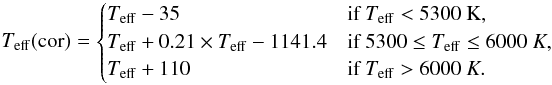
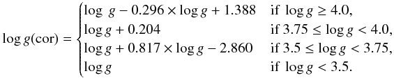
![Mathematical equation: \begin{eqnarray*} \text{[M/H]}({\rm cor}) &=& \text{[M/H]} + 0.15 \\ {}[\alpha\text{/Fe}]({\rm cor}) &=& [\alpha\text{/Fe}] \end{eqnarray*}](/articles/aa/full_html/2012/06/aa18829-12/aa18829-12-eq135.png) There are several potential sources of the bias corrections for the AMBRE:FEROS analysis. First, the differing techniques, as well as differing spectral domains and resolutions, used in the determination of the stellar parameters by the reference studies compared with AMBRE:FEROS analysis may make a significant contribution to the difference in derived parameters. Second, while the normalisation process within the AMBRE analysis pipeline was designed to be as robust as possible, the normalisation of stellar spectra is an inherently complex problem, particularly over large wavelength ranges with many spectral features. For spectra of particular spectral types (e.g. cool, low gravity, metal-rich) the normalisation procedure may not be as robust as for less detailed spectra. Third, due to the length of the atomic and molecular linelist that was required to synthesise the AMBRE:FEROS wavelength regions, it was inefficient to carry out a calibration of the linelist to standard stars (i.e. the Sun). It was assumed that the number of lines was statistically sufficient to dampen the noise from ill-fitted spectral features but non-calibration of the line list may play some role in the degree of the bias corrections. Individually, and in combination, these are the most likely sources of the bias corrections for the AMBRE:FEROS stellar parameters.
There are several potential sources of the bias corrections for the AMBRE:FEROS analysis. First, the differing techniques, as well as differing spectral domains and resolutions, used in the determination of the stellar parameters by the reference studies compared with AMBRE:FEROS analysis may make a significant contribution to the difference in derived parameters. Second, while the normalisation process within the AMBRE analysis pipeline was designed to be as robust as possible, the normalisation of stellar spectra is an inherently complex problem, particularly over large wavelength ranges with many spectral features. For spectra of particular spectral types (e.g. cool, low gravity, metal-rich) the normalisation procedure may not be as robust as for less detailed spectra. Third, due to the length of the atomic and molecular linelist that was required to synthesise the AMBRE:FEROS wavelength regions, it was inefficient to carry out a calibration of the linelist to standard stars (i.e. the Sun). It was assumed that the number of lines was statistically sufficient to dampen the noise from ill-fitted spectral features but non-calibration of the line list may play some role in the degree of the bias corrections. Individually, and in combination, these are the most likely sources of the bias corrections for the AMBRE:FEROS stellar parameters.
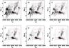 |
Fig. 15 HR diagrams of the FEROS stellar parameters as each rejection criterion is applied as follows: a) all spectra analysed in SPC; b) spectra with Vrad CCF with positive contrast, |

6.3. External error
The external error for each stellar parameter was determined from the above reference sample analysis. For each individual study the mean difference and spread in differences (σ) between the literature and AMBRE:FEROS values was calculated. The mean of these σ values for each stellar parameter was taken as the global external error (σ(θ)ext) for all of the spectra as follows: ![Mathematical equation: \begin{eqnarray*} && \sigma(T_{\rm eff})_{\rm ext} = 120 \text{~K} \\ && \sigma(\log \ g)_{\rm ext} = \begin{cases} 0.20 \text{~dex} &\text{if }\log g \geq 3.2,\\ 0.37 \text{~dex} &\text{if }\log g < 3.2,\\ \end{cases}\\ && \sigma(\text{[M/H]})_{\rm ext} = 0.10 \text{~dex} \\ && \sigma([\alpha/\text{Fe]})_{\rm ext} = 0.10 \text{~dex} \end{eqnarray*}](/articles/aa/full_html/2012/06/aa18829-12/aa18829-12-eq140.png) \arraycolsep1.75pt
\arraycolsep1.75pt
7. ESO table: rejection criteria
The construction of the ESO Table of stellar parameters that would be delivered to the ESO Archive was the final stage of the pipeline. At this stage the quality flags and tests included throughout the pipeline were drawn together to provide the final set of stellar parameters. The columns headings, their definitions, range of values, null values and rejection conditions used to construct the ESO Table are listed in Table A.1.
There were two phases of rejecting spectra in the AMBRE:FEROS analysis. First, prior to analysis in SPC spectra were rejected due to spectral quality issues. This will be described in the Sect. 7.1. Second, the remaining spectra were all analysed in SPC for their stellar parameters and then another set of rejection criteria were applied to construct the final table. These criteria are described and discussed in Sects. 7.2 to 7.4.
7.1. Pre-SPC: non-standard spectra
Prior to SPC, 11% of the FEROS archived spectra were rejected as being non-analysable primarily due to being non-standard spectra. The rejection flags, as defined in Sect. 4.1, were for “Faulty Spectra”, “Extreme Emission Features”, “Poor Normalisation” and “Excessive Noise”. Often the nature of a spectrum rejected at this stage meant the conditions for two or more of these flags were met. For instance, an extremely noisy spectrum was also consequently poorly normalised. Quality flags were also attached for “Large Emission Features” and “Instrumental Relics” but these spectra were not rejected based solely on these flags. The number of spectra identified for each rejection flag and for each quality flag are listed in Table 6.
Number of spectra rejected (Rej) prior to SPC based on the defined rejection flags and the number of spectra accepted (Acc) for SPC but identified by the quality flags.
7.2. Rejection criteria post-SPC
The remaining 89% of the FEROS spectra were analysed in SPC and so stellar parameters were obtained for each of these spectra. Figure 15a shows the HR diagram for all the stellar parameters obtained in SPC. The giant branch and main sequence can be observed but there is a great deal of mis-classification at hot temperatures for log g ≳ 2 dex, and an overdensity at Teff ≈ 3000 K and log g ≈ 2 dex. Most noticeable is that there are many spectra (8947) for which the derived parameters lie outside the Teff and log g grid limits which are indicated in red. In the construction of the ESO Table it would have been very straightforward to just reject all spectra whose parameters lay outside the limits of the synthetic grid and so only report to ESO those spectra with parameters inside the grid. However to have the synthetic grid limits as the sole reason to reject so many spectra (~47%) without further explanation seemed inadequate. Thus we further investigated the observational and astrophysical characteristics (indicators) of the spectra in order to better understand the dataset and to be able to impose more robust quality control criteria on the final dataset to be reported to ESO.
The SNR and log χ2 were investigated as potential indicators but both proved to be functions of spectral type (the more spectral features the lower the SNR, the poorer the observed to synthetic spectra fit) and the criteria rejected RGB stars rather than the high temperature mis-classifications.
Indicators relating to the measurement of the spectral FWHM and the radial velocity proved to be the least affected by spectral type and better identified the mis-classifications. The key indicators that were explored were: the Vrad CCF contrast, the error on the amplitude and the error on continuum of the Vrad CCF; the Vrad error; the FWHM of the Vrad CCF; the spectral FWHM; and the AMBRE:FEROS synthetic grid boundaries in Teff, log g, [M/H], [α/Fe].
Table 7 summarises the number of spectra that satisfied the conditions of each rejection criteria for the spectra rejected before and after SPC. The post-SPC rejection criteria were applied to the spectra rejected before SPC to further characterise that sample. To illustrate the effects of the rejection criteria on the sample of spectra analysed in SPC, Fig. 15 shows progressively the HR diagram of the AMBRE:FEROS stellar parameters as each criteria is applied. The limits of the synthetic grid in Teff and log g are also shown. This process is discussed in the following sections.
Summary of the number of spectra flagged as satisfying the conditions of the post-SPC rejection criteria.
7.2.1. CCF contrast, amplitude and continuum
As described in Sect. 4.2, the radial velocity was determined using binary masks to calculate a CCF. The contrast, the depth (amplitude) of the CCF, the continuum placement of the CCF and their associated errors (as calculated in the IDL:GAUSSFIT routine) are measures of the quality of the CCF. The rejection criteria were derived from these quantities as follows:
-
1.
A negative contrast means that the CCF profile is inverted,which is contrary to the expected result, hence all spectra with anegative contrast were rejected.
-
2.
The relative error on the amplitude of the CCF (
 ) is mainly a measure of how much noise there is in the CCF. If the
  then the noise makes up less than 20% of the profile depth. We rejected spectra with
  .
. -
3.
The placement of the continuum is also an indication of how well the CCF was defined. The relative error on the continuum (
 ) gives a measure of the noise in the continuum placement. We rejected all spectra with
  .
.
These three criteria identify spectra with poorly-defined CCFs. Combined they are the first criteria to be applied to the SPC dataset resulting in the rejection of a further 3668 spectra from the analysis. Figure 15b shows the resulting HR diagram after these spectra were removed. The hot star mis-classifications and overdensity at Teff ≈ 3000 K are diminished.
Figures 16a and b show histograms of the SNR per pixel (0.03 or 0.06 Å per pixel) for the full sample of FEROS archived spectra. The SNR has been calculated within the analysis pipeline using sigma clipping on either the predefined continuum regions in SPB or the pseudo-continuum residual in SPC. The highest SNR values do not necessarily mean optimum spectra and are identified by the quality flags within the pipeline as required. Figure 16a is the histogram of the spectra that were accepted as being of good quality and with a well-defined CCF, whereas Fig. 16b is the histogram of the spectra rejected as being of poor quality or with poorly-defined CCF. Note that the y-axis scale is different between the figures. The histogram in Fig. 16a peaks between 50 and 100 SNR. There are significantly fewer spectra with SNR < 50 in Fig. 16a compared with Fig. 16b, indicating the cleaning thus far has indeed identified low SNR spectra. However, as Figs. 10a to d shows, even at SNR of 50 the internal error is negligible.
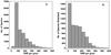 |
Fig. 16 Histogram of the measured SNR values of the FEROS archived spectra in bins of ΔSNR = 50: a) spectra defined as good quality and with well-defined CCFs (N = 15 513); b) spectra rejected as poor quality and/or poorly defined CCFS (N = 6038). The y-axes are to different scale to better display each sample. |
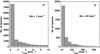 |
Fig. 17 Histogram of measured Vrad uncertainty for each of the FEROS archived spectra of good quality with a well-defined CCF. a) The distribution of the sample with σVrad < 10 km s-1. b) The distribution of the sample with σVrad > 10 km s-1. |
7.2.2. Vrad error
The next criterion to be applied was the Vrad error (σVrad) which had been calculated using the prescription in Tonry & Davis (1979). Figure 17 shows histograms of the σVrad determined for each of the FEROS archived spectra of good quality with a well-defined CCF. Figure 17a is a histogram of Vrad error < 10 km s-1 in bins of 1 km s-1, and Fig. 17b is a histogram of σVrad > 10 km s-1 in bins of 10 km s-1. The majority of the spectra have a low σVrad ( < 0.5 km s-1), and based on the synthetic spectra analysis in Sect. 4.2, Fig. 11 shows that ΔVrad ≤ 5 km s-1 correspond to reasonable variations in the stellar parameters (θ). However there are a significant number of spectra with σVrad greater than 10 km s-1 (see Fig. 17b) which correspond to much larger uncertainties in the θ determination.
Hence we decided to reject all spectra with σVrad > 10 km s-1. This resulted in a further 3550 spectra being rejected from the SPC dataset. The resulting HR diagram is shown in Fig. 15c. Again more of the mis-classifications at hot Teff, particular for high log g, have been removed and the overdensity at Teff ≈ 3000 K is considerably diminished.
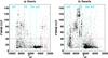 |
Fig. 18 Teff vs. FWHM of the CCF for a) giants (log g < 3.5 dex); b) dwarfs (log g ≥ 3.5 dex). The nominal temperature values for spectral types A0, F0, G0, K0 are shown as cyan lines. A CCF FWHM of 40 km s-1 is indicated in red. |
7.2.3. FWHM of Vrad CCF
Astrophysically, the FWHM of the Vrad CCF can be used to calculate the rotational velocity (Vsini) of a star. That particular calculation was not carried out here, for the purposes of expediency, but the FWHM of the CCF was used to identify spectra with broadened spectral features that would not be well represented by the synthetic grid. As discussed in Sect. 5.2, the synthetic spectra grid was generated with no variations in Vsini, assuming all stars to be slow rotators. The analysis in Gazzano et al. (2010) found that for a sample of FGK dwarfs Vsini < 11 km s-1 produced good results in the stellar parameter determination by MATISSE. At a resolution of R ~ 26 000 an upper limit of CCF FWHM = 20 km s-1 was set. Due to the lower resolution (R ~ 15 000), and hence greater masking of the effects of Vsini, of the AMBRE:FEROS analysis we sought to relax that criterion.
The comparison of spectral type with Vsini is used to show the increase in the number of fast rotators with hotter spectral type for both dwarfs and giants (see Chap. 18, Gray 2005). For dwarfs, fast rotators begin to appear at approximately F2 in spectral type, for giants at approximately G2. Using the stellar parameters derived in SPC and the spectral dataset that remained after the application of the σVrad rejection criterion, we replicated Spectral Type vs. Vsini using Teff and the CCF FWHM as proxies. The spectra were separated into subsamples of dwarfs and giants using the derived values for log g. The comparisons are shown in Figs. 18a and b.
The location of the Spectral Types in temperature are indicated (cyan lines). There is a clear dense grouping of spectra between 4000 and 6000 K with CCF FWHM less than 20 for both giants and dwarfs. Both samples have a great deal of scatter, particularly for Teff greater than 7000 K. Above the expected spectral type of F2 for the giants there is more dense scatter at higher CCF FWHMs. For the dwarfs the scatter becomes denser around 10 000 K. A CCF FWHM of 40 km s-1 is indicated in both cases (red line). This threshold was selected as being a factor of two greater than the threshold in Gazzano et al. (2010), as the resolution of the AMBRE:FEROS synthetic grid is approximately a factor of two lower in resolution than that study. Hence the astrophysical broadening is masked to at least a factor of 2 in the convolved FEROS spectra. Above the 40 km s-1 threshold the distribution of the points is sporadic while below this value the distribution is more coherent. However the majority of the points lie below 20 km s-1 in line with Gazzano et al. (2010). Ultimately we decided to reject all points with a CCF FWHM greater than 40 km s-1.
The effects of this cleaning on the HR diagram are shown in Fig. 15d. A significant number of mis-classifications with Teff > 7000 K have been removed as expected from the threshold shown in Fig. 18. These rejected stars should be analysed with a hotter synthetic spectra grid with variations in Vsini.
7.2.4. FWHM of the stellar spectrum
The calculation of the spectral FWHM was necessary in order to convolve the observed spectra to the resolution of the synthetic grid. However the FWHM values also provide an extra degree of information with which to understand the spectral dataset. The FWHM measurements were separated into FWHMweak, FWHMstrong and FWHMmedium classifications (Sect. 4.3). In particular the FWHMstrong classification allowed us to identify spectra with broad features, independantly of the FWHM of the Vrad CCF. For each FWHMstrong spectra, the FWHM of the medium strength lines was measured (where possible) as well as the FWHM of the identified strong lines. Figures 19a − c show the relationships between FWHMmedium and CCF FWHM, FWHMmedium and Teff, and FWHMstrong and Teff respectively for the dataset as of the application of the σVrad criterion.
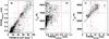 |
Fig. 19 Comparison of a) FWHMmedium with the CCF FWHM; b) Teff for the dataset with CCF FWHM < 40 km s-1 compared to the FWHMmedium; and c) as for b) but for FWHMstrong. Thresholds at CCF FWHM = 40 km s-1, FWHMmedium = 0.8 mÅ, FWHMstrong = 8 mÅ, and Teff = 7000 K are also shown. |
In Fig. 19a there is a clear trend of increasing CCF FWHM with FWHMmedium. The line at FWHMmedium = 0.8 mÅ intersects the trend at the threshold of CCF FWHM = 40 km s-1 where the trend becomes less dense. This provided the first criterion that we applied such that any spectra with a measured FWHMmedium greater than 0.8 mÅ were rejected.
Figure 15e shows the HR diagram after the removal of spectra based on this criterion. There is some improvement such that the density of the hot mis-classifications is decreased. However there are still a significant number of mis-classifications at temperatures greater than 7000 K. Further investigation showed that these remaining mis-classifications were connected to the “strong” FWHM classification (FWHMstrong).
There was no clear trend between the CCF FWHM and the FWHMstrong with which to derive a threshold of rejection. Instead a comparison was made to Teff. Figure 19b compares the Teff with the corresponding FWHMmedium. The lower boundary of possible values of Teff does increase with FWHMmedium and at the derived threshold of FWHMmedium = 0.8 mÅ this trend intersects with a Teff = 7000 K. For greater FWHMmedium values the trend of the lowest Teff disappears into greater scatter, essentially attributing a temperature value to the FWHMmedium threshold. This temperature value was used to infer a FWHMmedium threshold for the strong spectral lines.
Figure 19c shows the measured FWHMstrong (where possible) with the Teff. There is distinct trend of increasing temperature with increasing FWHMstrong. The nominal temperature threshold at 7000 K intersects with this trend at a FWHMstrong of 8 mÅ. At greater FWHMstrong there is an increase in scatter and the trend becomes more dispersed. The greater spread in values for spectra with FWHMstrong > 8 mÅ, and for FWHMmedium > 0.8 mÅ, may indicate a greater uncertainty in the parameterisation as the boundary of the grid is approached.
Based on this we can assume that spectra with a FWHMstrong not more than 8 mÅ have stellar parameters that fall within the synthetic grid and thus are well-defined. Hence this provided the second criterion to apply such that spectra with a FWHMstrong greater than 8 mÅ were rejected. Figure 15f shows that indeed the mis-classifications between 7000 K and 8000 K are significantly reduced after the application of this criterion.
7.3. Understanding the rejected spectra
Figure 20 explores the types of stars to which the 11 971 rejected spectra correspond. Figures 20a compares Teff with σVrad for the rejected sample. It is clearly bimodal with the primary peak at 8190 ± 924 K (10 068 spectra) and the secondary peak at 3351 ± 679 K (1903 spectra). The datasets corresponding to the key rejection criteria are also indicated: FWHMmedium rejections (pink), FWHMstrong rejections (yellow) and CCF FWHM rejections (cyan). The spectra rejected on the basis of FWHMmedium and FWHMstrong are concentrated in the two peaks. This argues that at least 84% of these spectra with broad features have returned parameters greater than the 8000 K temperature limit of the synthetic spectra grid.
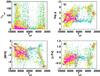 |
Fig. 20 Comparison of the Teff of the 11 971 rejected spectra (black) with a) σVrad; b) log g; c) [M/H] and d) [α/Fe]. The datasets for the FWHMmedium rejections (pink), FWHMstrong rejections (yellow) and CCF FWHM rejections (cyan) are shown. |
Figure 20b is the HR diagram of the rejected spectra. The majority have Teff > 6000 K, but also with log g > 2 dex implying these are sub-giants and dwarf stars. It is possible that these spectra have parameters that lie outside the available synthetic grid parameter space and MATISSE has compensated by varying one or all of the stellar parameters away from the true values in order to converge on a solution. Combined with the high number of these spectra that have been measured to have broadened spectral features, it is possible that these are in fact hot and/or fast rotating stars for which the synthetic grid has not been designed.
In Fig. 20a 16% of the rejected sample are located near the cool temperature limit of the synthetic grid (3351 ± 679 K). Are these truly such cool stars? Figure 20c compares the Teff with [M/H]. The cool temperature limit spectra show an interesting trend of decreasing [M/H] with decreasing temperature. For spectra with Teff < 3000 K the [M/H] extends significantly outside the grid range. A possible answer is that these are hot or fast rotating stars (based on the FWHM measurements) for which MATISSE has converged to a significantly cooler temperature with significantly decreased metallicity. A similar but less dramatic argument can be made for the spectra rejected at the hot temperature limit. These lie within the [M/H] range for the synthetic grid although many are metal-poor to − 3.5 dex. Combined with the high gravity values of these spectra the low metallicity emphasises the possiblity that these stars have been mis-classified due to their parameters lying outside the grid parameter space.
The comparison of [α/Fe] to Teff in Fig. 20d adds weight to this, as the cool temperature limit group have very high [α/Fe] values. For the hot temperature limit group the [α/Fe] are typically within the range of the synthetic grid.
From this examination of the key variables, the main argument that can be drawn as to why ~ 66.1% of the spectra analysed in SPC have been rejected by these very strict criteria is that they are most likely hot and/or fast rotating stars that are not well-represented by the current synthetic grid. Hence MATISSE has converged on solutions which mis-classify the spectra in the absence of a grid covering the required parameter range. This is not an unreasonable conclusion given that FEROS was designed and built by researchers within the hot star community (Kaufer et al. 1999). A visual inspection was carried out on large random samples of the spectra that were rejected based on each of the rejection criteria. This inspection supported the appropriate application of the criteria as the rejected spectra corresponded to noisy, peculiar or strong-lined spectra, and there was an over-representation of spectra comprising solely of strong balmer lines. However to confirm this conclusion these spectra can be re-analysed at a later date when a synthetic grid with Teff > 8000 K and a synthetic grid with a range in Vsini values will be available.
7.4. Synthetic grid boundaries
The above rejection criteria succeeded in cleaning the stellar parameter sample without losing the well-defined branches of stellar evolution that are observed in the HR diagram. Finally, the stellar parameters determined near the boundaries of the synthetic grid are inherently less reliable due to there being less synthetic spectra present to aid in the definition of the parameters. Hence the final rejection criteria that were applied are based on the stellar parameters themselves. Taking into account boundary effects in the learning phase of MATISSE, the limits on the accepted parameters are defined as follows: ![Mathematical equation: \begin{eqnarray*} 3000 &\leq& T_{{\rm eff}} \ \leq 7625 \\ 1 &\leq& \log g \ \leq \ 5 \\ -3.5 &\leq& \text{[M/H]} \ \leq \ 1 \\ -0.4 &\leq& [\alpha/\text{Fe}] \ \leq \ 0.4 \hspace{0.7cm} \text{if [M/H] }\geq 0.0 \\ -0.4 &\leq& [\alpha/\text{Fe}] \ \leq \ 0.8 \hspace{0.7cm} \text{if }-1.0 < [{\rm M/H}] < 0 \\ 0.0 &\leq& [\alpha/\text{Fe}] \ \leq \ 0.8 \hspace{0.7cm} \text{if }[{\rm M/H}] \leq -1. \end{eqnarray*}](/articles/aa/full_html/2012/06/aa18829-12/aa18829-12-eq173.png) Three categories were established using these definitions:
Three categories were established using these definitions:
-
1.
TON: Teff values only within the accepted limits;
-
2.
TGM: Teff, log g and [M/H] values within accepted limits;
-
3.
TGMA: Teff, log g, [M/H] and [α/Fe] within accepted limits.
The final count of spectra for these three categories were: TON = 394 spectra (~292 stars), TGM = 97 spectra (~87 stars), TGMA = 6017 spectra (~2780 stars).
In total 12 673 spectra were rejected from the SPC analysis. The final set of the stellar parameters accepted for delivery to ESO was comprised of 6508 spectra (~3087 stars). For the radial velocity analysis 11 963 spectra (~4505 stars) were determined to have radial velocities with σVrad ≤ 10 km s-1 and these values were also accepted for delivery to ESO. The full breakdown of the spectral number count is given in Table 8.
Number counts and percentages of spectra accepted (Acc.) or rejected (Rej.) during the AMBRE:FEROS analysis.
7.5. Repeated observations
The FEROS dataset contains many stars with repeated observations. Figure 21 shows histograms of the number of stars per number of observations for the TGMA sample. Figure 21a shows the histogram for the number of stars with observations less than or equal to 10, while Fig. 21b shows the number of stars with observations greater than 10. There is a significant number of stars with 2 or more observations, and some stars have been observed a great many times. The repeated observations were used to assess whether the AMBRE analysis derived consistent stellar parameters for the same star from different spectra.
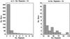 |
Fig. 21 Histogram of the humber of repeat observations in the TGMA sample for stars with: a) the number of observations less than or equal to 10; b) the number of observations greater than 10. |
All objects with 2 or more observations were extracted from the TGMA sample in order to explore the agreement in parameters for a single object over a number of observations of similar SNR. We also extracted from SIMBAD a list of objects within the FEROS dataset (based on a 10′′ coordinate search) that were designated as a binary and/or variable star. We found 17 binary stars and 111 variable stars in the final sample which we eliminated from the sample of repeat observations. Hence we removed those stars with possible astrophysical variations in the parameters to be left with variations that are solely due to the analysis process. (It must be noted that, as the list in SIMBAD is not exhaustive, it is likely that there are still stars for which the parameters vary astrophysically within the repeated observations sample.) The repeated observations sample was further constrained such that each set of repeats had a mean SNR less than 200, as the observations above SNR = 200 were sparcely sampled. Due to the prior application of the rejection criteria there were no spectra present with SNR < 40. Finally, the sample of repeats comprised of 584 stars equating to 3438 spectra. The maximum number of repeats was 73 for a single star in the repeats sample.
This sample represents the internal error of the AMBRE analysis hence we compared it to the internal error (σint) that we calculated for each spectra based on the SNR, Vrad and Normalisation (Sect. 5).
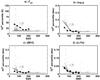 |
Fig. 22 Change in θ with SNR (in bins of 20) for the repeat observations within TGMA (black symbols) compared with the σ(θ)int values (Sect. 5) for TGMA (grey points). a) The ΔTeff that 70% of the repeat sample were less than or equal to at each SNR (black squares). The trend with SNR is shown by the black lines. b) As for a) but for variations in log g (black stars). c) As for a) but for variations in [M/H] (black circles). d) As for a) but for variations in [α/Fe] (black diamonds). |
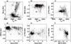 |
Fig. 23 The final FEROS stellar parameters for TGM (red) and TGMA (black) samples for a) The Hertzsrung-Russell diagram; b) [M/H] vs. Teff; c) [α/Fe] vs. Teff; d) [M/H] vs. log g; e) [α/Fe] vs. log g; f) [M/H] vs. [α/Fe]. |
Figure 22 replicates the relationships in Fig. 10 but for the repeats sample. For each set of repeats the mean and standard deviation were calculated for the SNR and stellar parameters. The standard deviation of each of the parameters was used to represent the change in the parameters (Δθ) for each set. The mean SNR values were binned (binsize = 25) and for each bin the 70th percentile of the Δθ was calculated. These values are shown in black. Also included in grey for each parameter are the internal errors calculated for the TGMA spectra (σ(θ)int, see Sect. 5).
In Fig. 22a the variations in Teff with SNR for the repeats sample is greater than the calculated internal error distribution and almost traces out the upper limit on the internal error. However, in general these two independant measurements of the internal error are on the same order of magnitude confirming the internal consistency within the AMBRE:FEROS analysis.
As defined in Sect. 5 the internal errors for log g, [M/H] and [α/Fe] are calculated as a piecewise function of SNR and this is reflected in the distribution of the internal errors for TGMA as shown in Figs. 22b to d. The lower limit of the internal errors for each of these three parameters decreases with increasing SNR to the defined constant value at SNR = 125. This distribution is replicated in the variation of each parameter with SNR for the repeats sample. At low SNR there is an offset in log g and [M/H] between the two sets of values where the internal errors are of greater value. This implies that the internal errors may be overestimated at low SNR in light of the repeats sample analysis. For [α/Fe] the variations due to the repeats sample trace the internal errors very well across the range of SNR values. But overall, as for Teff, these two independant measurements of the internal error for each parameter are in very good agreement.
The distribution of the variation of the parameters with SNR for the repeats sample in Fig. 22 also replicates the analysis of the internal error due to SNR that was carried out using the synthetic spectra sample as shown in Fig. 10. For the lowest SNR bin for each parameter the Δθ are only 2 or 3 times the equivalent value in the synthetic case which is reasonable, and as the SNR increases the Δθ decreases significantly also replicating the synthetic case.
The comparison between the two measures of the internal error from the observed spectra and with the synthetic spectra analysis shows that the analysis carried out within the pipeline is consistent such that closely comparable parameters are found for different spectra of the same star, and so for different stars of similar stellar parameters, at a particular SNR value.
8. The AMBRE:FEROS stellar parameters
The final FEROS stellar parameters are shown in Fig. 23 in six combinations with which to examine the distribution of the parameters.
Figure 23a shows the Hertzsprung-Russell (HR) diagram of the TGM (red) and TGMA (black) samples. The branches of stellar evolution are distinct although broad in width with some small scatter evident throughout the figure. Figure 23b compares [M/H] with Teff and the majority of the spectra show near solar metallicities ( − 1.0 < [M/H] < 0.5 dex) consistently across the temperatures.
Figure 23c compares [α/Fe] with Teff and shows an interesting distribution of low ( < 0.0 dex) and high ( > 0.2 dex) [α/Fe] at low temperatures but an even distribution of solar [α/Fe] across all temperatures.
Figure 23d compares [M/H] with log g and the separation between the giants and dwarfs is evident. There is larger scatter in [M/H] at low log g (giants).
Figure 23e compares [α/Fe] with log g and again the scatter is larger at low log g (giants).
Figure 23f compares [α/Fe] with [M/H] for which there is a clear trend of enhanced [α/Fe] (~0.35 dex) at low [M/H] ( < − 1.0 dex). For [M/H] of solar and above the [α/Fe] decreases to solar and depleted values.
Combining three parameters in one graph provides another perspective with which to further explore this dataset. Figure 24 shows the HR diagram of the TGM and TGMA samples binned by colour in [M/H]. The near solar [M/H] bins contain the majority of the sample as expected from Fig. 23 across the Main Sequence and RGB. The samples within the more metal-poor bins lie to the left of the stellar evolution branches which agrees with stellar evolutionary tracks. Interestingly the majority of the Horizontal Branch (HB) are metal-poor ([M/H] = − 1.62 dex).
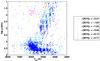 |
Fig. 24 The HR diagram of the TGM and TGMA FEROS stellar parameter samples binned by colour in [M/H]. The centre of each bin are listed in the legend. |
9. Conclusions and future work
The stellar parameterisation of the FEROS archive completes the first phase of the AMBRE Project. Of the 21 551 FEROS object spectra that were delivered to OCA, 19 181 could be analysed for their stellar parameters. The quality flags and error analysis resulted in a final total of 6508 spectra (~3087 stars) with stellar parameters to be delivered to ESO. Also delivered to ESO are the radial velocity values for 11 963 spectra (~4505 stars).
Approximately 70% of the spectra were rejected from the stellar parameterisation analysis. While 28% were rejected due to the quality of the spectra being insufficient for analysis, 42% were rejected due to astrophysical reasons. From this analysis it seems very likely that hot and/or fast rotating stars are the favoured observational object for FEROS. As the current synthetic grid is defined for stars cooler than 8000 K only then the high number of rejections was inevitable. In general the AMBRE synthetic spectra grid is currently configured for slow-rotating FGK stars. Non-standard stars, such as binaries and chemically peculiar stars, within the FEROS sample may still pollute the final accepted dataset as we were unable to identify such stars at this stage.
However, stellar parameter extensions to the synthetic spectra grid are under development and identification tools are also being developed such that a larger range of spectra may be reliably analysed at a later date.
In summary the work carried out in the analysis of the FEROS archived spectra has resulted in:
-
1.
The development of a complex and robust analysis pipeline forthe determination of stellar parameters of large spectral datasetsthrough automated iterative spectral reduction andMATISSE analysis.
-
2.
The establishment of tools with which to exploit spectral atlases and libraries for the comprehensive testing and validation of the results from the AMBRE analysis pipeline.
-
3.
The determination of stellar parameters (Teff, log g, [M/H], [α/Fe]) for 6508 of 21 551 FEROS archived spectra to be made available in the ESO Archive, including quality flags.
-
4.
The determination of radial velocities (Vrad) for 11 963 of 21 551 FEROS archived spectra to be made available in the ESO Archive.
The AMBRE pipeline is currently being used to determine stellar parameters for the UVES and HARPS archived spectra, the next two phases of analysis in the AMBRE Project. The analysis of the FLAMES/GIRAFFE archived spectra is expected to commence in early 2012.
Acknowledgments
The AMBRE Project team members would like to thank ESO, OCA and CNES for their financial support of this project. We would like to thank the referee for the constructive comments on this paper. We would also like to thank O. Begin, Y. Vernisse, S. Rousset and F. Guitton for their work on the development of the AMBRE analysis pipeline as well as the OCA Mesocentre members. We would like to thank C. Soubiran and T. Bensby for proving stellar parameters and spectra for testing the pipeline. We would like to thank B. Plez for the use of Turbospectrum and the molecular linelists, and also C. Melo for the use of the radial velocity programme. Thanks also to L. Pasquini for initiating the project, and to M. Romaniello and J. Melnich for their help within ESO. This research has made use of the SIMBAD database, operated at CDS, Strasbourg, France, as well as the NASA/IPAC Infrared Science Archive, which is operated by the Jet Propulsion Laboratory, California Institute of Technology, under contract with the National Aeronautics and Space Administration.
References
- Allen de Prieto, C. 2003, MNRAS, 339, 1111 [NASA ADS] [CrossRef] [Google Scholar]
- Allen de Prieto, C., Barklem, P. S., Lambert, D. L., & Cunha, K. 2004, A&A, 420, 183 [NASA ADS] [CrossRef] [EDP Sciences] [Google Scholar]
- Alonso, A., Arribas, S., & Martinez-Roger, C. 1996, A&AS, 117, 227 [NASA ADS] [CrossRef] [EDP Sciences] [Google Scholar]
- Alonso, A., Arribas, S., & Martínez-Roger, C. 1999, A&AS, 139, 335 [NASA ADS] [CrossRef] [EDP Sciences] [Google Scholar]
- Alvarez, R., & Plez, B. 1998, A&A, 330, 1109 [NASA ADS] [Google Scholar]
- Bagnulo, S., Jehin, E., Ledoux, C., et al. 2003, The Messenger, 114, 10 [NASA ADS] [Google Scholar]
- Barden, S. C., Jones, D. J., Barnes, S. I., et al. 2010, SPIE Conf. Ser., 7735 [Google Scholar]
- Bensby, T., Feltzing, S., & Lundström, I. 2003, A&A, 410, 527 [NASA ADS] [CrossRef] [EDP Sciences] [Google Scholar]
- Bijaoui, A., Recio-Blanco, A., & de Laverny, P. 2008, AIP Conf. Ser. 1082, ed. C. A. L. Bailer-Jones, 54 [Google Scholar]
- Blackwell, D. E., & Lynas-Gray, A. E. 1998, A&AS, 129, 505 [NASA ADS] [CrossRef] [EDP Sciences] [Google Scholar]
- Brault, & Neckel, 1999, Sol. Phys., 184, 421 [NASA ADS] [CrossRef] [Google Scholar]
- Crifo, F., Jasniewicz, G., Soubiran, C., et al. 2010, A&A, 524, A10 [NASA ADS] [CrossRef] [EDP Sciences] [Google Scholar]
- de Laverny, P., Recio-Blanco, A., Worley, C. C., & Plez, B. 2012, A&A, submitted [arXiv:1205.2270] [Google Scholar]
- Dekker, H., D’Odorico, S., Kaufer, A., Delabre, B., & Kotzlowski, H. 2000, SPIE Conf. Ser. 4008, ed. M. Iye, & A. F. Moorwood, 534 [Google Scholar]
- Delbouille, L., Roland, G., & Neven, L. 1973, Atlas photometrique DU spectre solaire de [lambda] 3000 a [lambda] 10 000 [Google Scholar]
- di Benedetto, G. P. 1998, A&A, 339, 858 [NASA ADS] [Google Scholar]
- Fuhrmann, K. 1998a, A&A, 338, 161 [NASA ADS] [Google Scholar]
- Fuhrmann, K. 1998b, A&A, 330, 626 [NASA ADS] [Google Scholar]
- Fuhrmann, K. 2004, Astron. Nachr., 325, 3 [NASA ADS] [CrossRef] [MathSciNet] [Google Scholar]
- Fuhrmann, K. 2008, MNRAS, 384, 173 [NASA ADS] [CrossRef] [Google Scholar]
- Fuhrmann, K., Pfeiffer, M., Frank, C., Reetz, J., & Gehren, T. 1997, A&A, 323, 909 [NASA ADS] [Google Scholar]
- Fuhrmann, K., Pfeiffer, M. J., & Bernkopf, J. 1998, A&A, 336, 942 [NASA ADS] [Google Scholar]
- Gazzano, J.-C., de Laverny, P., Deleuil, M., et al. 2010, A&A, 523, A91 [NASA ADS] [CrossRef] [EDP Sciences] [Google Scholar]
- González Hernández, J. I., & Bonifacio, P. 2009, A&A, 497, 497 [NASA ADS] [CrossRef] [EDP Sciences] [Google Scholar]
- Gratton, R. G. 1989, A&A, 208, 171 [NASA ADS] [Google Scholar]
- Gratton, L., Gaudenzi, S., Rossi, C., & Gratton, R. G. 1982, MNRAS, 201, 807 [NASA ADS] [Google Scholar]
- Gratton, R. G., Carretta, E., & Castelli, F. 1996, A&A, 314, 191 [NASA ADS] [Google Scholar]
- Gratton, R. G., Carretta, E., Claudi, R., Lucatello, S., & Barbieri, M. 2003, A&A, 404, 187 [NASA ADS] [CrossRef] [EDP Sciences] [Google Scholar]
- Gray, D. F. 2005, The Observation and Analysis of Stellar Photospheres, 3rd edn. (Cambridge, UK: Cambridge University Press) [Google Scholar]
- Gustafsson, B., Edvardsson, B., Eriksson, K., et al. 2008, A&A, 486, 951 [NASA ADS] [CrossRef] [EDP Sciences] [Google Scholar]
- Hekker, S., & Meléndez, J. 2007, A&A, 475, 1003 [NASA ADS] [CrossRef] [EDP Sciences] [Google Scholar]
- Hinkle, K., Wallace, L., Valenti, J., & Harmer, D. 2000, Visible and Near Infrared Atlas of the Arcturus Spectrum 3727 − 9300 A [Google Scholar]
- Kaufer, A., Stahl, O., Tubbesing, S., et al. 1999, The Messenger, 95, 8 [Google Scholar]
- Kordopatis, G., Recio-Blanco, A., de Laverny, P., et al. 2011, A&A, 535, A106 [NASA ADS] [CrossRef] [EDP Sciences] [Google Scholar]
- Kovtyukh, V. V., Soubiran, C., Belik, S. I., & Gorlova, N. I. 2003, A&A, 411, 559 [NASA ADS] [CrossRef] [EDP Sciences] [Google Scholar]
- Kovtyukh, V. V., Soubiran, C., & Belik, S. I. 2004, A&A, 427, 933 [NASA ADS] [CrossRef] [EDP Sciences] [Google Scholar]
- Kovtyukh, V. V., Soubiran, C., Bienaymé, O., Mishenina, T. V., & Belik, S. I. 2006, MNRAS, 371, 879 [NASA ADS] [CrossRef] [Google Scholar]
- Kupka, F., Piskunov, N., Ryabchikova, T. A., Stempels, H. C., & Weiss, W. W. 1999, A&AS, 138, 119 [NASA ADS] [CrossRef] [EDP Sciences] [MathSciNet] [PubMed] [Google Scholar]
- Kurucz, R. L. 1979, ApJS, 40, 1 [NASA ADS] [CrossRef] [Google Scholar]
- Luck, R. E., & Bond, H. E. 1983, ApJ, 271, L75 [Google Scholar]
- Luck, R. E., & Bond, H. E. 1991, ApJS, 77, 515 [NASA ADS] [CrossRef] [Google Scholar]
- Luck, R. E., & Heiter, U. 2005, AJ, 129, 1063 [NASA ADS] [CrossRef] [Google Scholar]
- Luck, R. E., & Heiter, U. 2006, AJ, 131, 3069 [NASA ADS] [CrossRef] [Google Scholar]
- Majewski, S. R., Skrutskie, M. F., Schiavon, R. P., et al. 2007, BAAS, 39, 962 [NASA ADS] [Google Scholar]
- Masana, E., Jordi, C., & Ribas, I. 2006, A&A, 450, 735 [NASA ADS] [CrossRef] [EDP Sciences] [Google Scholar]
- Mayor, M., Pepe, F., Queloz, D., et al. 2003, The Messenger, 114, 20 [NASA ADS] [Google Scholar]
- McWilliam, A. 1990, ApJS, 74, 1075 [NASA ADS] [CrossRef] [Google Scholar]
- Melo, C. H. F., Pasquini, L., & De Medeiros, J. R. 2001, A&A, 375, 851 [NASA ADS] [CrossRef] [EDP Sciences] [Google Scholar]
- Mishenina, T. V., & Kovtyukh, V. V. 2001, A&A, 370, 951 [NASA ADS] [CrossRef] [EDP Sciences] [Google Scholar]
- Mishenina, T. V., Kovtyukh, V. V., Korotin, S. A., & Soubiran, C. 2003, Astron. Rep., 47, 422 [Google Scholar]
- Mishenina, T. V., Soubiran, C., Kovtyukh, V. V., & Korotin, S. A. 2004, A&A, 418, 551 [NASA ADS] [CrossRef] [EDP Sciences] [Google Scholar]
- Mishenina, T. V., Bienaymé, O., Gorbaneva, T. I., et al. 2006, A&A, 456, 1109 [NASA ADS] [CrossRef] [EDP Sciences] [Google Scholar]
- Mishenina, T. V., Soubiran, C., Bienaymé, O., et al. 2008, A&A, 489, 923 [NASA ADS] [CrossRef] [EDP Sciences] [Google Scholar]
- Palacios, A., Gebran, M., Josselin, E., et al. 2010, A&A, 516, A13 [NASA ADS] [CrossRef] [EDP Sciences] [Google Scholar]
- Pasquini, L., Avila, G., Blecha, A., et al. 2002, The Messenger, 110, 1 [NASA ADS] [Google Scholar]
- Ramírez, I., & Meléndez, J. 2005, ApJ, 626, 446 [Google Scholar]
- Ramírez, I., Allen de Prieto, C., & Lambert, D. L. 2007, A&A, 465, 271 [NASA ADS] [CrossRef] [EDP Sciences] [Google Scholar]
- Recio-Blanco, A., Bijaoui, A., & de Laverny, P. 2006, MNRAS, 370, 141 [NASA ADS] [CrossRef] [Google Scholar]
- Soubiran, C., Le Campion, J., Cayrel de Strobel, G., & Caillo, A. 2010, A&A, 515, A111 [NASA ADS] [CrossRef] [EDP Sciences] [Google Scholar]
- Steinmetz, M., Zwitter, T., Siebert, A., et al. 2006, AJ, 132, 1645 [NASA ADS] [CrossRef] [Google Scholar]
- Tonry, J., & Davis, M. 1979, AJ, 84, 1511 [NASA ADS] [CrossRef] [Google Scholar]
- Valenti, J. A., & Fischer, D. A. 2005, ApJS, 159, 141 [NASA ADS] [CrossRef] [MathSciNet] [Google Scholar]
- Wallace, L., Hinkle, K., & Livingston, W. 1998, An atlas of the spectrum of the solar photosphere from 13 500 to 28 000 cm-1 (3570 to 7405 A) (Tucson, AZ: National Optical Astronomy Observatories) [Google Scholar]
- Yanny, B., Rockosi, C., Newberg, H. J., et al. 2009, AJ, 137, 4377 [NASA ADS] [CrossRef] [Google Scholar]
Appendix A: Description of ESO Table for AMBRE:FEROS
Description of columns in the table of FEROS stellar parameters delivered to ESO.
All Tables
Details of the four ESO spectrographs and their publicly available archived spectra sample that are part of the AMBRE Project.
FEROS échelle order, starting wavelength and finishing wavelength for each region used in the analysis of the FEROS spectra.
List of the stellar parameters for the binary masks used in the AMBRE:FEROS radial velocity determination that were built from the full AMBRE synthetic grid (45 masks) and the POLLUX database (6 masks).
List of standard stars and the corresponding spectral atlases used to test the FEROS analysis pipeline.
List of spectral libraries used to select comparison stars from the FEROS archived spectra.
Number of spectra rejected (Rej) prior to SPC based on the defined rejection flags and the number of spectra accepted (Acc) for SPC but identified by the quality flags.
Summary of the number of spectra flagged as satisfying the conditions of the post-SPC rejection criteria.
Number counts and percentages of spectra accepted (Acc.) or rejected (Rej.) during the AMBRE:FEROS analysis.
Description of columns in the table of FEROS stellar parameters delivered to ESO.
All Figures
|
Fig. 1 Number of FEROS observations per year for analysis in AMBRE. The 2005 observations begin in October. The number of distinct objects observed and the number with repeated observations are as indicated in the key. |
| In the text | |
|
Fig. 2 Bθ(λ) sensitivity: number of extrema above 2σ in ~ 200 Å bins against wavelength for four sets of stellar parameters: the Sun; Teff = 6000 K, log g = 2, [M/H] = 0.0; Arcturus; and Teff = 4500 K, log g = 4, [M/H] = −0.5. The Bθ(λ) vectors from left to right are: θ = Teff, log g and [M/H]. The grey stripes represent the final wavelength regions selected for the AMBRE:FEROS analysis (see Table 2). |
| In the text | |
|
Fig. 3 As for Fig. 2 but for the corresponding Bθ(λ) vectors of the AMBRE:FEROS synthetic spectra grid. The y-axis is scaled down compared to Fig. 2. |
| In the text | |
|
Fig. 4 The FEROS Analysis Pipeline: the key stages are displayed in order of analysis. Spectral Processing A and Spectral Processing B carry out testing of spectra quality and preliminary parameter determination, including calculation of the radial velocity and spectral FWHM. In Spectral Processing C robust iterative procedures are carried out resulting in the final stellar parameters and normalised spectra. See text for detailed explanation of each stage. |
| In the text | |
|
Fig. 5 CCFs produced for calculating radial velocities. a) Noisy CCF with an asymmetric profile. b) Core of profile showing skewed full profile gaussian fit (black). The secondary gaussian fit (red) provides a better estimate. c) CCF of the spectroscopic binary, HD 135728, showing two profiles. |
| In the text | |
|
Fig. 6 Examples of cross-correlation functions of the best fit masks for three of the FEROS spectra. The first row shows the full CCFs while the second row shows the profiles from which the radial velocities were determined. The final AMBRE:FEROS stellar parameters (Teff,log g, [M/H], [α/Fe]) and radial velocities are stated for each spectrum. The red lines are used to calculate the contrast and FWHM for each profile. |
| In the text | |
|
Fig. 7 Comparison of AMBRE:FEROS radial velocities: a) S4N library for 29 stars (338 spectra); and b) Crifo et al. (2010) for 158 stars (318 spectra). |
| In the text | |
|
Fig. 8 Histogram of the radial velocity values calculated for all of the FEROS archived spectra defined as good spectra with well-defined CCFs: a) Vrad; and b) FWHM of the Vrad CCF. |
| In the text | |
|
Fig. 9 Normalisation procedure for a two stars with Teff ~ 4600 K (left) and Teff ~ 5300 K (right) shown by the wavelength region about two lines of the magnesium triplet. Top: the second iteration of SPB, middle: first iteration of SPC, and bottom: final solution from SPC. The stellar parameters (Teff, log g, [M/H] and [α/Fe]) and goodness of fit over all the AMBRE:FEROS wavelengths (log χ2) are shown. The synthetic spectrum interpolated to these parameters is shown in red, while the normalised observed spectrum is shown in black. The difference between observed and synthetic spectra is also shown at 0.0. |
| In the text | |
|
Fig. 10 Internal error for each parameter with changes in SNR. a) The ΔTeff that 70% of the synthetic sample were less than or equal to when calculating the difference between the nominal Teff and the Teff determined for the respective SNR. b) As for a) but for log g. c) As for a) but for [M/H]. d) As for a) but for [α/Fe]. |
| In the text | |
|
Fig. 11 Internal error for each parameter with changes in the Vrad uncertainty (km s-1). a) The ΔTeff that 70% of the synthetic sample were less than or equal to when calculating the difference between the nominal Teff and the Teff determined for the respective Vrad uncertainty. b) As for a) but for log g. c) As for a) but for [M/H]. d) As for a) but for [α/Fe]. |
| In the text | |
|
Fig. 12 Box & Whisker graph of the absolute difference in the log χ2 of the reconstructed to the normalised spectra for the 384 test spectra between the 9th SPC iteration and each of the previous iterations ( | log χ2(9) − log χ2(i) | ). The box is constrained by the 25th and 75th percentiles, and the red lines are the medians. The whiskers extend to the furthest data points not considered to be outliers. |
| In the text | |
|
Fig. 13 Internal error with changes in Normalisation for a) Teff; b) log g; c) [M/H]; and d) [α/Fe]. The red lines are determined as the 2σ uncertainty on values in two SNR bins (ΔSNR ≈ 30) centred at SNR = 65 and 100 and constant uncertainty for SNR > 125. |
| In the text | |
|
Fig. 14 Comparison of stellar parameters determined in AMBRE:FEROS (A:F) and the reference sample (RS) from PASTEL: a) Teff; b) log g; c) [M/H] compared with [Fe/H]; d) [α/Fe]. The legend identifies the relevant individual papers and the associated sample bias ± σ. The stellar atlases are also shown. The dashed line indicates a 1:1 agreement. The axis limits represent the limits on the final accepted parameters. |
| In the text | |
|
Fig. 15 HR diagrams of the FEROS stellar parameters as each rejection criterion is applied as follows: a) all spectra analysed in SPC; b) spectra with Vrad CCF with positive contrast, |
| In the text | |
|
Fig. 16 Histogram of the measured SNR values of the FEROS archived spectra in bins of ΔSNR = 50: a) spectra defined as good quality and with well-defined CCFs (N = 15 513); b) spectra rejected as poor quality and/or poorly defined CCFS (N = 6038). The y-axes are to different scale to better display each sample. |
| In the text | |
|
Fig. 17 Histogram of measured Vrad uncertainty for each of the FEROS archived spectra of good quality with a well-defined CCF. a) The distribution of the sample with σVrad < 10 km s-1. b) The distribution of the sample with σVrad > 10 km s-1. |
| In the text | |
|
Fig. 18 Teff vs. FWHM of the CCF for a) giants (log g < 3.5 dex); b) dwarfs (log g ≥ 3.5 dex). The nominal temperature values for spectral types A0, F0, G0, K0 are shown as cyan lines. A CCF FWHM of 40 km s-1 is indicated in red. |
| In the text | |
|
Fig. 19 Comparison of a) FWHMmedium with the CCF FWHM; b) Teff for the dataset with CCF FWHM < 40 km s-1 compared to the FWHMmedium; and c) as for b) but for FWHMstrong. Thresholds at CCF FWHM = 40 km s-1, FWHMmedium = 0.8 mÅ, FWHMstrong = 8 mÅ, and Teff = 7000 K are also shown. |
| In the text | |
|
Fig. 20 Comparison of the Teff of the 11 971 rejected spectra (black) with a) σVrad; b) log g; c) [M/H] and d) [α/Fe]. The datasets for the FWHMmedium rejections (pink), FWHMstrong rejections (yellow) and CCF FWHM rejections (cyan) are shown. |
| In the text | |
|
Fig. 21 Histogram of the humber of repeat observations in the TGMA sample for stars with: a) the number of observations less than or equal to 10; b) the number of observations greater than 10. |
| In the text | |
|
Fig. 22 Change in θ with SNR (in bins of 20) for the repeat observations within TGMA (black symbols) compared with the σ(θ)int values (Sect. 5) for TGMA (grey points). a) The ΔTeff that 70% of the repeat sample were less than or equal to at each SNR (black squares). The trend with SNR is shown by the black lines. b) As for a) but for variations in log g (black stars). c) As for a) but for variations in [M/H] (black circles). d) As for a) but for variations in [α/Fe] (black diamonds). |
| In the text | |
|
Fig. 23 The final FEROS stellar parameters for TGM (red) and TGMA (black) samples for a) The Hertzsrung-Russell diagram; b) [M/H] vs. Teff; c) [α/Fe] vs. Teff; d) [M/H] vs. log g; e) [α/Fe] vs. log g; f) [M/H] vs. [α/Fe]. |
| In the text | |
|
Fig. 24 The HR diagram of the TGM and TGMA FEROS stellar parameter samples binned by colour in [M/H]. The centre of each bin are listed in the legend. |
| In the text | |
Current usage metrics show cumulative count of Article Views (full-text article views including HTML views, PDF and ePub downloads, according to the available data) and Abstracts Views on Vision4Press platform.
Data correspond to usage on the plateform after 2015. The current usage metrics is available 48-96 hours after online publication and is updated daily on week days.
Initial download of the metrics may take a while.